Utility of low-cost sensor measurement for predicting ambient PM_2.5 concentrations: evidence from a monitoring network in Accra, Ghana

Abstract

Ambient air pollution has been linked to several health endpoints. The WHO attributes 7 million deaths annually to air pollution with particulate matter (PM_2.5) being the pollutant of critical importance due to its devastating health effects. Air quality monitoring is very limited in sub-Saharan African (SSA) countries and although satellite remote sensing has helped to bridge the huge air quality data gaps, these measurements have not been validated against ground-level measurements in these countries. We therefore evaluated the efficiency of low-cost sensors in estimating PM_2.5 concentrations in an African city through comparison of low-cost sensor data with satellite aerosol optical depth (AOD) data leveraging complex machine learning (ML) methods. Low-cost sensor data were collected from a monitoring network in Accra, Ghana, with AOD measurements extracted from the MODIS MCD19A2v061 dataset and processed using the MAIAC algorithm. Ordinary Least Squares regression, Random Forest, Extra Trees, Boosted Decision Trees and XGBoost were used to establish the relationship between AOD and low-cost sensor PM_2.5 measurements incorporating meteorological data. We observed significant positive relationships for two low-cost sensors deployed in the network (Clarity Node S and Airnote). The R² values were, however, low, ranging from 0.18 to 0.27, with the corrected Airnote data recording the highest R². The ML models which integrated temperature and humidity improved the R² values with the Boosted Decision Tree demonstrating the best predictive capability. Seasonal variability was found to have a strong influence on model performances with the dry season model performing significantly better than the wet season model. Consistent with other studies, AOD explained only a small proportion of ground-level PM_2.5 variations. Evidence from this sensor network in Accra suggests that AOD predicts ground-level PM_2.5 measured with low-cost sensors in a manner similar to conventional air monitoring instrumentation. However, for low-cost sensors to be deemed a good substitute for satellite AOD, data correction with complex algorithms developed in the same research location will be required.

---

Environmental significance

Emerging low-cost air quality sensors have the potential to help bridge the huge air quality data gaps in sub-Saharan African (SSA) countries. The reliability of satellite-derived PM_2.5 estimates for SSA countries has not been established owing to limited ground monitoring instrumentation. The study findings have important implications for PM_2.5 exposure estimation in LMICs where satellite AOD is heavily relied upon due to limited ground monitoring. Low-cost sensors are being widely adopted in these countries and for PM_2.5 measurements from these sensors to be deemed a good substitute for satellite AOD, data correction using complex algorithms developed in the same research location will be required, accounting for meteorological factors, spatial information and several other factors. Correction factors developed in one geographical location should therefore not be applied to low-cost data collected in another geographical location.

Introduction

There is mounting evidence linking ambient air pollution exposure with several health endpoints including respiratory infections, chronic obstructive pulmonary disease (COPD), cardiovascular diseases, lung cancer, and adverse birth outcomes.^1–5 The World Health Organization (WHO) estimates that air pollution contributes to 7 million deaths worldwide annually.⁶ Particulate matter (PM), comprising solid and liquid substances suspended in the air is the most monitored and regulated air pollutant globally. This is because it is one of the six criteria pollutants that countries are mandated to monitor and also because it is the pollutant with the strongest causal evidence for adverse health impacts. The detrimental effects of PM are largely attributed to fine (PM_2.5) and ultra-fine (PM_1.0) particles possessing the ability to penetrate deep into the respiratory and cardiovascular system, thereby inducing acute and chronic health effects. PM can also exert significant health effects even at low levels of exposure.^7,8 The health consequences are even more pronounced in low-income countries and communities where they can interact with socioeconomic risk factors.⁹

Air quality in sub-Saharan African (SSA) cities has deteriorated due to rapid population growth and urbanization in these areas which has led to increased vehicle ownership, widespread use of solid fuels for cooking and heating, and poor waste management practices, coupled with industrial expansion.¹⁰ Some of the highest fine particles levels in the world have been recorded in SSA cities and other developing regions, with PM_2.5 concentrations in SSA cities estimated at around 100 μg m⁻³ compared to <20 μg m⁻³ in most European and North American cities.¹¹

In spite of such disparities, SSA countries have very limited air quality monitoring capacity. In the past few decades, satellite aerosol remote sensing has become increasingly valuable for improving the estimation of ground-level PM_2.5,^12,13 especially in areas with limited monitoring capacity. This is because satellite measurements offer wide spatial coverage that cannot be matched by any ground monitoring network. Satellite-based monitoring does, however, have limitations. Ground-level PM concentrations are monitored on a continuous scale whereas aerosol optical depth (AOD) is retrieved only when the satellite passes overhead, typically once per day (overpass hour) and therefore cannot represent the diurnal variability at monitoring locations. Also, satellite data are available on clear days with cloudiness masking retrieval abilities and resulting in substantial missing data due to cloud cover and high surface reflectance. In addition, the relationship between AOD and ground-level PM_2.5 depends on numerous factors including aerosol vertical profile, water content, size distribution, and composition.¹⁴ Reliable data on several of these factors are, however, not available at large spatial scales and require the use of statistical models and chemical transport models^15,16 to establish the relationship. The use of these models also has shortcomings and further adds to the uncertainty.^13,16,17 These factors likely explain the wide variability observed in the literature regarding the estimated relationship between AOD and ground-level PM_2.5.

Emerging low-cost air quality sensors have the potential to help bridge the huge air quality data gaps in SSA countries by providing access to air quality data with high spatiotemporal resolution while overcoming the limitations of satellite measurements. Air pollution measurements at high spatiotemporal resolution are necessary for an accurate assessment of exposure. This, however, requires the deployment of low-cost sensors at several locations to increase granularity in the air pollution measurement, i.e., ubiquitous monitoring. Low-cost sensors also have the potential to advance exposure science by complementing regulatory monitoring to enable better characterization of air pollution exposure, a major validity concern in air pollution epidemiologic studies. Moreover, while global estimation models of PM_2.5 using AOD have been developed, the reliability of satellite-derived PM_2.5 estimates remains highly uncertain in SSA countries which have sparse coverage of conventional air monitoring to validate such estimates.¹⁸

Given the limitations of satellite remote sensing in estimating PM_2.5 concentrations in areas with sparse air quality monitoring, it is essential to assess the potential of low-cost sensors as an alternative method for evaluating air quality exposure in these regions. Such evidence will make air quality data readily available, more reliable, and accessible in real-time for public awareness creation and to inform air pollution policy decisions. Aainst this background, we are leveraging data from a low-cost sensor monitoring network in Accra (https://breatheaccra.org/) to evaluate the utility of low-cost sensor measurement and satellite aerosol optical depth data for estimating PM_2.5 concentrations in a SSA city with limited air quality monitoring capacity.

Methods

Low-cost PM_2.5 sensor data

The Breathe Accra project (https://breatheaccra.org/) is a hyperlocal low-cost air sensor monitoring network in Accra, with sensors deployed in thirteen beneficiary districts of the Greater Accra Metropolitan Area (GAMA). In this project, surface PM_2.5 data are collected using Clarity Node S¹⁹ and Airnote.²⁰ We combined data from Clarity Node S and Airnote as both use similar types of internal Plantower sensors. Sensors with data available from March 2023 to August 2024 (25 sensors) were selected from the network for the study. Measurement data from the sensors were recorded every 15 minutes. The data were split into wet and dry season measurements. The wet season spanned from March to October 2023 with the dry season spanning from November 2023 to February 2024. Fig. 1 illustrates the geographical boundaries of the 13 beneficiary districts and the locations where the sensors are located within the districts. Selecting sites for placement of the sensors was influenced by structures in the community with sensors mounted in hospitals, schools, market centers, bus terminals and lorry stations, roadside and traffic hotspots, and residential neighborhoods of varying socioeconomic status.

Fig. 1 Map of the study area and sensor deployment locations.

Satellite data retrieval

The satellite data product used in this paper is the MODIS MCD19A2v061 dataset²¹ available through NASA's Earth Data Portal.²² Aerosol Optical Depth (AOD) measurements were performed at wavelengths of 470 nm and 550 nm using the data product. These data are processed using the Multi-Angle Implementation of Atmospheric Correction (MAIAC) algorithm and subsequently presented at a spatial resolution of 1 km per pixel for each overpass of either the Aqua or Terra satellite platforms.^21,23 The MAIAC algorithm was selected for processing these data due to its advanced capabilities in aerosol retrieval, cloud detection and atmospheric correction which significantly improve the accuracy of satellite-derived surface reflectance and AOD. Unlike traditional atmospheric correction methods, MAIAC employs a time-series analysis approach combined with a multi-angle processing strategy to dynamically model the surface bidirectional reflectance distribution function (BRDF) and aerosol properties.^24,25 Additionally, MAIAC utilizes an adaptive cloud mask and an improved aerosol retrieval scheme that can separate fine and coarse aerosol modes, leading to more reliable atmospheric correction compared to earlier algorithms like Dark Target (DT) or Deep Blue (DB).²⁵ By leveraging multi-angle observations from the Moderate Resolution Imaging Spectroradiometer (MODIS) onboard the Aqua and Terra satellites, MAIAC can account for directional surface reflectance effects, reducing uncertainties in atmospheric correction. This results in more accurate surface reflectance products, which are essential for climate studies, land cover classification, and air quality monitoring.²⁴ Extraction of the dataset was performed by employing the Google Earth Engine platform. Based on the MCD19A2 user manual, only AOD measurements categorized under the “best quality” assurance criteria were included, with cloudy pixels being appropriately masked out.

The satellite AOD measurements have very high spatial resolution and a wide monitoring range²⁶ and were therefore considered to be collocated with the low-cost sensors within a 1 km × 1 km grid cell. Low-cost sensors within these grid cells of the satellite AOD data were compared. To ensure alignment of the low-cost sensor measurements with the MODIS Terra and Aqua measurements, we included only measurements that were taken within a ±15 minute interval of the overpass time of the two satellites. The overpass times of the two satellites were considered independent of each other and hence, daily averages of the measurement obtained from the two satellites were not computed. Therefore, for most days we obtained two AOD readings, one from Terra and one from Aqua. The satellite AOD data were retrieved based on the geolocation and position of each low-cost sensor to ensure alignment between both datasets. The start date of each retrieval was based on the date of sensor deployment and continued until March, 2024. Fig. 2 shows the air pollution heat map for the study area during the study period as estimated by the low-cost sensors and the AOD extracted from the satellites.

Fig. 2 PM_2.5 concentrations estimated from the low-cost sensors (left pane) and satellite aerosol optical depth (right pane).

Data processing

Based on the MCD19A2 user guidelines, cloudy pixels were masked out and only AOD considered as best quality was retrieved using the Google Earth Engine Editor. Both wavelengths were correlated and hence, we chose the 550 nm optical depth band for the analysis. For AODs extracted at the Airnote locations, Pearson's correlation coefficient was 0.997 and for AODs extracted at the Clarity Node locations, Pearson's correlation coefficient was 0.998. PM_2.5 measurements from the low-cost sensors within a ±15 minute interval of the Tera (10:30 am) and Aqua (1:30 pm) overpass times were used. As a result, low-cost measurements without corresponding satellite AODs were excluded and vice versa. Outliers in each dataset were removed using the Interquartile range (IQR) approach. Fig. 3 and 4 show a boxplot of the PM_2.5 measurements from the Airnote and Clarity sensors, respectively, recorded at monitoring locations. From Table 1, the total percentage of PM_2.5 and AOD matchups for the Clarity and Airnote sensors was 14.6% and 8.7%, respectively. Table 2 presents summary statistics of the PM_2.5 data gathered from the sensors. PM_2.5 measurements recorded from the Clarity S-Node sensor were corrected using a correction factor (eqn (1)) developed by Raheja and colleagues.²⁷ There are no correction factors developed for the Airnote sensor in this region and hence we could not correct for this data.

Corrected PM_2.5 = 54.6 + 0.4 × reported PM_2.5 − 0.76 × temp. (°C) − 0.35 × reported RH (%) (1)

Table 1 Comparison of PM_2.5 measurements from Clarity and Airnote sensors with MODIS satellite data during overpass time^a

Sensor type	Total PM2.5 measurement	Paired PM2.5 measurement with MODIS optical depth	Percentage difference
a Average number of days for each sensor (Clarity = 469, Airnote = 384).
Clarity	11 278	1642	14.6%
Airnote	9979	823	8.2%

---

Fig. 3 PM_2.5 measurements recorded by the Airnote sensor at the deployment locations.

Fig. 4 PM_2.5 measurements recorded by the Clarity S Node sensor at the deployment locations.

Table 2 Summary statistics of PM_2.5 measurements from the low-cost sensors

Sensor type	Mean	Standard deviation	Lower quartile (Q1)	Upper quartile (Q3)	Interquartile range (IQR)
Clarity – uncorrected	31.59	18.27	16.38	43.80	27.42
Clarity – corrected	20.30	8.37	13.61	25.45	11.84
Airnote	25.08	16.11	11.45	35.65	24.19

---

Estimating PM_2.5 from satellite aerosol optical depth (AOD)

Ordinary Least Squares (OLS) regression was used to estimate the relationship between AOD and ground level PM_2.5. The core assumption is that there exists a linear relationship between AOD and PM_2.5 spatially and temporally.²³ The regression coefficients β₀ and β₁ are optimized in the linear regression using the OLS approach.

The regression analysis will generate a linear equation of the form:

PM_2.5 = β₀ + β₁ (AOD 550 nm) + ε (2)

where β₀ is the y-intercept, β₁ is the slope of the line, and ε is the error term accounting for any unexplained variation. AOD values are the independent variable and PM_2.5 is the dependent variable. A linear regression model was fitted between the PM_2.5 and each AOD wavelength. Once the model was trained, the equation was used to predict the PM_2.5 from the test AOD data.

To enhance the accuracy of the estimation process, advanced modelling techniques were employed. The models integrated meteorological data including temperature and humidity together with spatial data captured by the low-cost sensors (LCSs). Various models were employed including OLS regression for establishing linear relationships and non-parametric machine learning models – Random Forest, Extra Trees, Boosted Decision Trees and XGBoost to help establish non-linear relationships.^28,29

The relationship for PM_2.5 concentration measured by LCSs is modelled as:

PM_2.5 [LCS] = f(AOD 550 nm, temperature [LCS], humidity [LCS], geolocation [LCS]) (3)

A Random Forest constitutes an ensemble of decision trees trained on diverse subsets of training data. Each decision tree within the forest is constructed using distinct feature subsets and varying training data subsets. In this study, the RandomForestRegressor from the sklearn.ensemble library module in Python was employed. This methodology generates an ensemble of decision trees characterized by diversity and low correlation, thereby enhancing model accuracy and ability to capture complex interactions between predictors.^30–32

The Extremely Randomized Trees (Extra-Trees) model, similar to Random Forests, leverages an ensemble of decision trees for supervised learning tasks. However, it introduces a key distinction by introducing additional randomization during the feature selection and splitting processes. Unlike Random Forests, which meticulously search for the optimal split at each node, the Extra-Trees algorithm introduces randomness by selecting a random subset of features and subsequently choosing a split point from this subset.³³ This additional level of randomness leads to the creation of more diversified trees within the ensemble, potentially leading to improved generalizability on specific datasets especially when dealing with noisy features.^31,34 A Boosted Decision Tree model, AdaBoostRegressor from the sklearn.ensemble library in python was also employed. Initially, a base decision tree regressor is trained on the entire dataset. Subsequent trees are then sequentially trained, with each tree focusing on correcting the errors of its predecessors by assigning higher weights to instances that were poorly predicted. This weight adjustment process is controlled by a learning rate parameter, which determines the contribution of each tree to the final ensemble.^35,36 By combining multiple weak learners, the ensemble gradually improves its ability to generalize to unseen data. The final prediction is made by aggregating the predictions of all trees in the ensemble, typically weighted according to their individual performance. This iterative boosting procedure not only enhances predictive power but also fosters robustness against overfitting, making it a popular choice in various regression tasks where both accuracy and interpretability are critical.³⁷

Additionally, we examined the implementation of XGBoost as a form of gradient boosting. Unlike the bagging approach employed in Random Forest and Extra-Trees, each new tree is designed to rectify the errors of the preceding trees.^38,39 XGBoost accomplishes this through gradient boosting which involves fitting new models to the negative gradient of the loss function. This enables the ensemble to learn from the mistakes of earlier models. This iterative approach often yields superior predictive accuracy, albeit at the cost of reduced model interpretability compared to individual decision trees.^38,40 Both Clarity Node S dataset and Airnote dataset were split into 80% training data and 20% test data for all modeling. The chosen machine learning models were based on their wide applicability in similar studies conducted previously. In these studies, the norm was to deploy a number of machine learning algorithms to identify the best performing model.

Evaluation of model performance

To assess model performance, we employed three commonly used metrics in regression analysis and machine learning: coefficient of determination (R²), Root Mean Squared Error (RMSE), and Mean Absolute Error (MAE). R² quantifies the proportion of variance in the observed data that is explained by the model. An R² value closer to 1 indicates that a large proportion of variability in PM_2.5 is captured by the model. The RMSE measures the average magnitude of the prediction errors, expressed in the same units as the target variable (μg m⁻³). RMSE is particularly useful because the squaring the errors penalizes larger deviations more strongly, making it sensitive to outliers. Lower RMSE values indicate better model performance. The MAE calculates the average absolute difference between the observed and predicted values. Unlike RMSE, MAE treats all errors equally, making it more robust to outliers. MAE provides a straightforward interpretation of the average error magnitude. Using these three metrics together enables a comprehensive evaluation of the models. While R² provides insight into the overall explanatory power of the model, RMSE and MAE quantify the average prediction errors. This combination helps to better understand both the variance explained by the model and the typical error magnitude in our PM_2.5 estimations.

Statistical analysis

Python and QGIS v3.38.0 were used for running the models with the following libraries: numpy: 2.1.0, pandas: 2.2.2, matplotlib: 3.9.1, seaborn: 0.13.2, statsmodels: 0.14.4, sklearn: 1.5.1, xgboost: 2.1.2, geopandas: 1.0.1, shapely: 2.0.5, rasterio: 1.3.10.

Results

Table 3 presents the results from the OLS regression models for predicting PM_2.5 concentrations using AOD at 550 nm, for the entire data, and for dry and wet season measurements. The overall β coefficients were 19.41(95% CI: 17.21, 22.26), 8.58 (95% CI: 7.56, 9.59) and 20.04 (95% CI: 17.43, 22.65), for uncorrected Clarity data, corrected Clarity data and Airnote data, respectively. The model explained 18.2% to 27.0% of the variance in PM_2.5 with the Airnote data recording the highest R² value (27.0%). The RMSE values ranged from 7.50 to 16.59 with the corrected Clarity data recording the lowest prediction error (7.50). The dry season effect sizes were larger than the wet season effect sizes. Low R² and high RMSE values were recorded in both models. However, the dry season model appears to perform better with the larger R² values compared to the wet season model.

Table 3 Ordinary Least Squares (OLS) regression prediction (PM_2.5 measurements – aerosol optical depth at 550 nm)

	Overall			Dry season			Wet season
	Clarity (uncorrected data)	Clarity (corrected data)	Airnote	Clarity (uncorrected data)	Clarity (corrected data)	Airnote	Clarity (uncorrected data)	Clarity (corrected data)	Airnote
β coefficient (95% CI)	19.41 (17.21, 22.26)	8.58 (7.56, 9.59)	16.18 (14.85, 17.49)	32.47 (28.82, 36.11)	17.16 (15.40, 18.92)	26.50 (22.29, 30.71)	1.93 (−4.44, 8.29)	−0.64 (−3.27, 2.00)	9.85 (2.35, 17.35)
R-squared	0.196	0.182	0.27	0.304	0.345	0.315	0.00007	0.0005	0.015
Adjusted R squared	0.196	0.181	0.27	0.303	0.344	0.313	−0.00132	−0.0015	0.013
RMSE	16.59	7.50	14.22	16.34	7.95	13.08	12.92	5.29	10.32

---

Tables 4–6 present the performance metrics of the five machine learning models deployed on the Airnote data, uncorrected Clarity data, and corrected Clarity data, respectively, accounting for temperature and humidity. The tables present the results of these machine learning models for predicting PM_2.5 concentrations using the overall data, and dry and wet season measurements. For all three datasets (Airnote, and uncorrected and corrected Clarity data), the Boosted Decision Tree model showed the best predictive performance with the lowest RMSE and MAE values and the highest R² values. The Random Forest and XGBoost performed moderately well for all three datasets with the Multiple Linear Regression recording the poorest performance with the highest RMSE values and the lowest R² values. The performance of the models on the dry season data was much better than on the wet season data, and was somehow comparable to the overall data.

Table 4 Performance metrics of machine learning models deployed on Airnote PM_2.5 measurement

Model	Overall				Dry season				Wet season
	RMSE	MAE	R ^2	Adjusted R^2	RMSE	MAE	R ^2	Adjusted R^2	RMSE	MAE	R ^2	Adjusted R^2
Multiple Linear Regression	13.52	10.91	0.43	0.41	12.76	10.28	0.42	0.38	10.74	8.92	0.073	0.029
Random Forest	12.38	9.29	0.52	0.50	12.04	8.62	0.48	0.45	9.74	7.58	0.238	0.201
Extra Trees	12.75	9.57	0.49	0.47	12.71	9.05	0.42	0.39	9.98	7.45	0.216	0.179
Boosted Decision Tree	12.35	9.62	0.52	0.51	11.57	8.35	0.52	0.49	10.02	7.79	0.193	0.156
XGBoost	13.52	10.51	0.41	0.39	10.73	8.92	0.54	0.51	11.28	8.52	−0.022	−0.071

---

Table 5 Performance metrics of machine learning models deployed on uncorrected Clarity PM_2.5 measurement

Model	Overall				Dry season				Wet season
	RMSE	MAE	R ^2	Adjusted R^2	RMSE	MAE	R ^2	Adjusted R^2	RMSE	MAE	R ^2	Adjusted R^2
Multiple Linear Regression	16.03	12.71	0.20	0.19	6.15	4.77	0.53	0.52	5.00	3.90	0.070	0.030
Random Forest	15.75	12.18	0.31	0.30	5.31	3.99	0.65	0.64	4.61	3.56	0.21	0.18
Extra Trees	15.46	11.72	0.27	0.26	5.46	4.21	0.63	0.62	5.24	3.96	−0.066	−0.022
Boosted Decision Tree	14.39	11.26	0.43	0.43	5.07	3.84	0.68	0.67	4.47	3.51	0.26	0.23
XGBoost	15.37	11.85	0.30	0.29	5.63	4.27	0.61	0.59	4.92	3.72	0.102	0.064

---

Table 6 Performance metrics of machine learning models deployed on corrected Clarity PM_2.5 measurement

Model	Overall				Dry season				Wet season
	RMSE	MAE	R ^2	Adjusted R^2	RMSE	MAE	R ^2	Adjusted R^2	RMSE	MAE	R ^2	Adjusted R^2
Multiple Linear Regression	6.41	5.09	0.38	0.37	15.37	11.93	0.32	0.29	12.51	9.75	0.007	−0.035
Random Forest	6.34	4.89	0.45	0.44	13.14	9.86	0.50	0.48	11.59	8.86	0.15	0.11
Extra Trees	6.22	4.69	0.40	0.40	13.63	10.44	0.46	0.45	13.25	10.02	−0.11	−0.16
Boosted Decision Tree	5.86	4.54	0.55	0.55	12.76	9.67	0.53	0.51	11.73	9.34	0.13	0.089
XGBoost	6.33	4.87	0.46	0.45	13.51	10.62	0.43	0.42	12.24	9.32	0.05	0.009

---

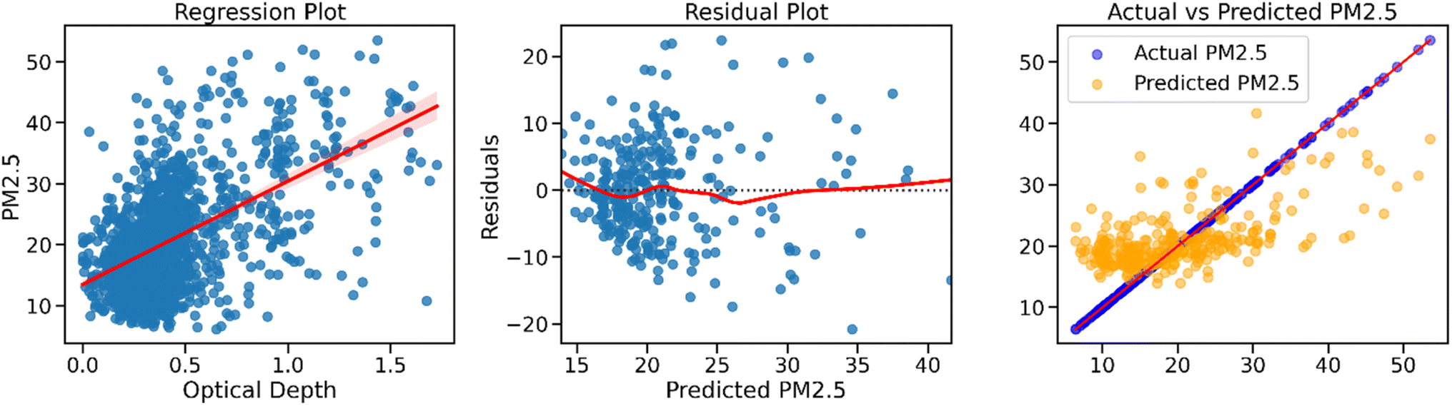
Fig. 5–7 present the scatter plot of Airnote, uncorrected Clarity and corrected Clarity PM_2.5 measurements, and AOD, respectively. In all the figures, the regression plot in the left pane shows a positive relationship between PM_2.5 and AOD but the data points are highly scattered, indicating a weak linear fit. The residual plots in the middle pane exhibit a pattern deviating significantly from randomness. The plot in the right pane compares the actual PM_2.5 measurements with the predicted values and shows that the predicted PM_2.5 values do not align with the actual PM_2.5 values. The plots for the dry and wet season measurements show similar patterns (Fig. S1–S6†).

Fig. 5 Scatter plot of overall Airnote PM_2.5 measurements and aerosol optical depth at 550 nm.

Fig. 6 Scatter plot of overall uncorrected Clarity PM_2.5 measurements and aerosol optical depth at 550 nm.

Fig. 7 Scatter plot of overall corrected Clarity PM_2.5 measurements and aerosol optical depth at 550 nm.

Discussion

Using the OLS regression model, we investigated the relationship between AOD retrieved from MODIS and PM_2.5 measurements from two different low-cost sensors (Clarity Node S and Airnote) deployed in our Breathe Accra project in Accra, Ghana. We found statistically significant positive relationships between AOD and PM_2.5 measurements from both sensors. A one-unit increase in satellite AOD increased low-cost senor PM_2.5 measurements by 19.41 μg mg⁻³, 8.58 μg m⁻³ and 16.28 μg m⁻³ for uncorrected Clarity data, corrected Clarity data and Airnote data, respectively. However, the low R² values (18–27%) observed suggest that the proposed model does not improve prediction over the mean model as AOD explains a small proportion of the variation in the low-cost sensor PM_2.5 measurements. A high proportion of the variance remains unexplained and hence the results should be interpreted with caution. The R² for the corrected data was slightly lower than that for the uncorrected data. However, the RMSE values for the corrected data were much smaller than those for the uncorrected data. With RMSE being the most important criterion for checking model fitting of prediction models, it therefore appears that correcting the data improved the prediction model. The residual plots in Fig. 5–7 exhibit a pattern deviating significantly from randomness, which suggests that the linear model does not fully capture the underlying relationship between the variables. The plots in the right panes of Fig. 5–7 compare the actual PM_2.5 measurements with the predicted values and show that the predicted PM_2.5 values do not align with actual PM_2.5 values. This suggests that, the model can predict the PM_2.5 measurements accurately. Collectively, these figures underscore the limitations of the current linear modeling approach in capturing the underlying relationship between PM_2.5 and AOD under different measurement conditions. The low R² for OLS regression and significant residual patterns, suggest limited model reliability. Separating the data into dry and wet season measurements does not also improve the model, with the wet season model performing poorly. Temporal or seasonal variability cannot therefore be a reason for the poor performance of the overall model but possibly, lack of control of important meteorological factors such as wind speed, and land cover/use factors which have been identified in several studies^41,42 as crucial for improving model performance. We did not have access to this data and hence could not incorporate them into the model.

AOD represents integration of the entire atmospheric column whereas ground-level PM concentrations represent breathing zone measurements. AOD therefore signifies greater attenuation of light by atmospheric particles which potentially includes PM_2.5.^31,43 Furthermore, AOD accounts for the influence of water vapor and coarse particles whereas PM_2.5 primarily indicates the dry mass concentration of tiny particulate matter and is not affected by any of the two factors.^44–46 It is important to establish the relationship between ground-level PM_2.5 and satellite AOD to better understand PM_2.5 exposure experiences of populations in LMICs where ground-monitoring is very limited and satellite AOD has been widely applied for exposure estimation. This investigation has become even more important with the recent influx of low-cost air quality sensors and their widespread adoption in LMICs to bridge the huge air quality data gaps as well as, the increasing need for air pollution data for epidemiologic research as indicated by Amegah.⁴⁷

Studies using PM_2.5 data from reference-grade monitors have also reported weak to moderate correlations between MODIS AOD to ground level PM_2.5^44,45,48 with OLS regression used to fit the data. It therefore likely that OLS regression is not the best model to examine the relationship between PM_2.5 and AOD. The residual plot of regression suggests some degree of non-linearity in the data. We therefore leveraged ensemble modelling techniques while including meteorological factors as inputs.

A number of studies have investigated the relationship between AOD and ground-level PM^23,46,49,50 and observed positive findings as seen in our study. However, with our finding of AOD explaining only a small proportion of the variation in PM_2.5 data (i.e., low R² values), it highlights the need to consider other factors in the prediction of ground-level PM_2.5 from satellite AOD. Studies using reference-grade monitoring data indicated that ground-level PM_2.5 and AOD vary greatly including spatially and as a result correlation between the two parameters is not always strong.^51,52

Meteorological factors are well documented to play a significant role in air quality assessment and estimation. Accounting for temperature and humidity in the OLS regression increased the R² values and decreased the RMSE values. For the corrected Clarity data, the R² and RMSE values were 0.38 and 6.41, respectively, representing a very substantial change (>100% change for both values). Using other machine learning models and accounting for temperature, humidity, and spatial information which was captured in the geographical coordinates also increased the R² values. The Boosted Decision Tree was found to have the best predictive accuracy compared to the other machine learning methods. The R² and RMSE values from this model increased and decreased substantially, respectively. This finding could be due to the Boosted Decision Tree's ability to capture and build sequentially, and also address the limitations of previous decision trees while maintaining control over overfitting.^53,54 XGBoost is generally considered to have superior performance compared to the Boosted Decision Tree. However, for smaller or medium-sized datasets like ours, it has been reported that the additional complexity of the model introduces redundant overhead thereby enabling the simpler Boosted Decision Tree to perform better^55,56 as seen in our study. In similar studies,^{37,38,40,57,58} Random Forest and XGBoost were found to have the highest R² values and lowest RMSE. The complexity of machine learning models allows for feature engineering of multiple variables, capturing both linear and non-linear relationships and hence incorporating all forms of relationships into the model. This enables machine learning techniques to improve model prediction, hence unsurprising that accounting for temperature, humidity and spatial information improved the model's prediction performance compared to the OLS regression. Several studies have also identified other factors that can also improve model prediction performance for better estimation of PM_2.5. Wind speed and direction, visibility, air pressure, dew point, precipitation, altitude, land use information (e.g., population density) and other pollutant gases like NO₂, SO₂ and CO have been reported to improve model performance when incorporated into the models.^28,39,57,59 These pollutant gases have also been observed to influence the satellite AOD either directly through the formation of sulfate and nitrate aerosols or indirectly by altering the atmospheric conditions.^60,61

We observed significant seasonal variations in the results. The models perform significantly better during the dry season compared to the wet season. For example, in Airnote data (Table 4), Multiple Linear Regression recorded an R² of 0.42 for dry season measurements compared to 0.073 for wet season measurements. This disparity likely arises from seasonal meteorological differences. Stable atmospheric conditions (e.g., lower humidity and reduced precipitation) during the dry season allow pollutants like PM_2.5 to accumulate, creating clearer spatial and temporal patterns for models to learn.⁶² With less cloud cover during this period, AOD retrieval from the MAIAC tends to be more precise.²⁷ However, it should also be noted that during the dry season dust storms from the Saharan desert have been recorded to travel south thereby increasing the concentration and magnitude of aerosols in the region.^63–65 Also, rainfall and higher humidity disrupt PM_2.5 concentrations through wet deposition and increased particle coagulation, introducing noise that linear models struggle to capture.^62–66 The widespread adoption of low-cost sensors in LMICs presents significant challenges due to the need for calibration against reference-grade monitors. In this study, we applied a correction factor developed by Raheja and colleagues from a study conducted in Accra, Ghana,²⁷ which is the same location as our study. Calibration functions which are typically established at a single reference station are prone to systematic errors when applied to other locations due to variations in atmospheric composition and meteorological conditions.^67–69 This situation should, however, not be a problem in our study because Raheja et al.'s study and our study were conducted at the same location. As a result, the atmospheric composition and meteorological conditions are not expected to be very different even though the two studies were conducted at different time points. The correction factor is therefore suitable for application to our low-cost sensor data. However, the reliability of data adjustment algorithms for low-cost sensors remains uncertain. The correction factor was suited for wet season measurements as Raheja and colleagues excluded the dry season measurements in the development of the correction factor. The authors explained that they were unable to collocate the sensors during the dry season.²⁷ However, we applied the correction factor to our entire data which incorporates dry season measurements and hence subject to some degree of measurement error. We found that the machine learning models performed better on the corrected data compared to the uncorrected data (Tables 5 and 6), possibly confirming the efficiency of the correction factor. However, it is also possible that, the measurement error overestimated the performance of the models. To mitigate the measurement error, we adhered to Raheja and colleagues'²⁷ recommendation to use the MLR correction factor instead of the tree-based methods which are prone to estimating PM_2.5 poorly outside the training data. These emerging methodologies raise critical questions regarding the transferability of sensor calibrations across space and time, the optimal parameters for data post-processing, and the extent to which corrected sensor data can be considered independent measurements rather than model outputs.^70,71 While optical particle sensors indirectly determine particulate matter mass concentration by measuring light scattering intensity, the complex relationship between light scattering and particle properties, including density, hygroscopicity, refractive index and composition renders mass concentration estimates sensitive to spatial and temporal variations.^71–73

Conclusion

In OLS regression we found satellite derived AOD not to be a very good predictor of ground-level PM_2.5 measurements obtained from low-cost sensors even after correction using calibration equations developed from data collected from the same research location and accounting for meteorological factors and spatial information. Deploying other machine learning techniques, we found that the Boosted Decision Tree improved model prediction. The findings of this study highlight three issues. Firstly, ground level PM_2.5 is influenced by several factors besides meteorological data and hence complex modelling techniques need to be employed to guarantee highly accurate predictive models. Secondly, algorithms for the correction of low-cost sensor data need to be evaluated for applicability in studies to ensure validity of the corrected data. Finally, seasonal variability has a strong influence on ground-level PM_2.5 prediction and should be considered in predictions of this nature to enhance accuracy and precision of the prediction model. The study's findings have important implications for PM_2.5 exposure estimation in LMICs where satellite AOD is heavily relied upon due to limited ground monitoring. Low-cost sensors are being widely adopted in these countries and for PM_2.5 measurements from these sensors to be deemed a good substitute for satellite AOD, data correction with complex algorithms developed in the same research location is required, accounting for meteorological factors, spatial information and several other factors. Correction factors developed in one geographical location should therefore not be applied to low-cost data collected from another geographical location.

Abbreviations

SSA	Sub-Saharan Africa
PM2.5	Particulate matter of less than 2.5 micrometers in diameter
AOD	Aerosol optical depth
MAIAC	Multi-angle implementation of atmospheric correction
MODIS	Moderate resolution imaging spectroradiometer

Data availability

All data underlying the findings of the study are available upon reasonable request from the corresponding author.

Conflicts of interest

There are no conflicts to declare.

Acknowledgements

The study was funded by the Clean Air Fund under the Breathe Accra: Data Component Project (Grant number: 001298) and the National Institute of Environmental Health Sciences of the National Institutes of Health under Award Number U01ES036147. The content of this article is solely the responsibility of the authors and does not necessarily represent the official views of the National Institutes of Health and Clean Air Fund. We are extremely grateful to the 13 beneficiary assemblies of the Breathe Accra Project whose support enabled us to set up the low-cost sensor monitoring network.

References

1. H.-B. Kim, J.-Y. Shim, B. Park and Y.-J. Lee, Long-Term Exposure to Air Pollutants and Cancer Mortality: A Meta-Analysis of Cohort Studies, Int. J. Environ. Res. Public Health, 2018, 15(11), 2608.
2. A. Gupta, A. Singh, B. Tarimci, A. K. Sindhu, P. Bathvar, S. Bedi, N. W. Y. Theik, V. Shah, S. Malhotra, M. Khealani, S. U. J. Obulareddy, G. Kukreja and A. Kanitkar, PM 2.5 and risk of lung cancer and associated mortality: An umbrella meta-analysis, J. Clin. Oncol., 2024, 42, e20012.
3. D. Zhang, W. Chen, C. Cheng, H. Huang, X. Li, P. Qin, C. Chen, X. Luo, M. Zhang, J. Li, X. Sun, Y. Liu and D. Hu, Air pollution exposure and heart failure: A systematic review and meta-analysis, Sci. Total Environ., 2023, 872, 162191.
4. J. Yanhui, L. Zhennan, H. Zhi, L. Chenyang, Z. Youjing, W. Jingyu, L. Fangchao, L. Jianxin, H. Keyong, C. Jie, G. Xinyuan, L. Xiangfeng and C. Shufeng, Effect of Air Pollution on Heart Failure: Systematic Review and Meta-Analysis, Environ. Health Perspect., 2024, 131, 76001.
5. L.-Q. Guo, Y. Chen, B.-B. Mi, S.-N. Dang, D.-D. Zhao, R. Liu, H.-L. Wang and H. Yan, Ambient air pollution and adverse birth outcomes: a systematic review and meta-analysis, J. Zhejiang Univ. – Sci. B, 2019, 20, 238–252.
6. WHO, Compendium of WHO and Other UN Guidance on Health and Environment: 2022 Update, WHO Fact Sheet, 2022, vol. 2019, p. 5.
7. J. S. Apte, J. D. Marshall, A. J. Cohen and M. Brauer, Addressing Global Mortality from Ambient PM2.5, Environ. Sci. Technol., 2015, 49, 8057–8066.
8. M. L. Bell, K. Ebisu and K. Belanger, Ambient Air Pollution and Low Birth Weight in Connecticut and Massachusetts, Environ. Health Perspect., 2007, 115, 1118–1124.
9. Q. Di, Y. Wang, A. Zanobetti, Y. Wang, P. Koutrakis, C. Choirat, F. Dominici and J. D. Schwartz, Air pollution and mortality in the Medicare population, N. Engl. J. Med., 2017, 376, 2513–2522.
10. A. K. Amegah and S. Agyei-Mensah, Urban air pollution in Sub-Saharan Africa: Time for action, Environ. Pollut., 2017, 220, 738–743.
11. M. Brauer, M. Amann, R. T. Burnett, A. Cohen, F. Dentener, M. Ezzati, S. B. Henderson, M. Krzyzanowski, R. V Martin, R. Van Dingenen, A. van Donkelaar and G. D. Thurston, Exposure Assessment for Estimation of the Global Burden of Disease Attributable to Outdoor Air Pollution, Environ. Sci. Technol., 2012, 46, 652–660.
12. J. Bi, J. H. Belle, Y. Wang, A. I. Lyapustin, A. Wildani and Y. Liu, Impacts of snow and cloud covers on satellite-derived PM2.5 levels, Rem. Sens. Environ., 2019, 221, 665–674.
13. Q. Di, I. Kloog, P. Koutrakis, A. Lyapustin, Y. Wang and J. Schwartz, Assessing PM2.5 Exposures with High Spatiotemporal Resolution across the Continental United States, Environ. Sci. Technol., 2016, 50, 4712–4721.
14. C. Lin, Y. Li, Z. Yuan, A. K. H. Lau, C. Li and J. C. H. Fung, Using satellite remote sensing data to estimate the high-resolution distribution of ground-level PM2. 5, Rem. Sens. Environ., 2015, 156, 117–128.
15. C. J. Paciorek, Y. Liu, H. Moreno-Macias and S. Kondragunta, Spatiotemporal Associations between GOES Aerosol Optical Depth Retrievals and Ground-Level PM2.5, Environ. Sci. Technol., 2008, 42, 5800–5806.
16. A. van Donkeelar, R. V. Martin, M. Brauer, R. Kahn, R. Levy, C. Verduzco and P. J. Villeneuve, Global Estimates of Ambient Fine Particulate Matter Concentrations from Satellite-Based Aerosol Optical Depth: Development and Application, Environ. Health Perspect., 2010, 118, 847–855.
17. G. Geng, Q. Zhang, R. V Martin, A. van Donkelaar, H. Huo, H. Che, J. Lin and K. He, Estimating long-term PM2. 5 concentrations in China using satellite-based aerosol optical depth and a chemical transport model, Rem. Sens. Environ., 2015, 166, 262–270.
18. A. van Donkelaar, M. S. Hammer, L. Bindle, M. Brauer, J. R. Brook, M. J. Garay, N. C. Hsu, O. V Kalashnikova, R. A. Kahn, C. Lee, R. C. Levy, A. Lyapustin, A. M. Sayer and R. V Martin, Monthly Global Estimates of Fine Particulate Matter and Their Uncertainty, Environ. Sci. Technol., 2021, 55, 15287–15300.
19. Low-Cost Air Quality Monitoring & Measurement | Clarity Movement Co., 2024, https://www.clarity.io/.
20. Airnote – Blues Developers, 2019, https://dev.blues.io/datasheets/airnote-datasheet/airnote-v2-0/.
21. Y. Lyapustin and A. Wang, MODIS/Terra+Aqua Land Aerosol Optical Depth Daily L2G Global 1km SIN Grid V061 [Data Set], NASA EOSDIS Land Processes Distributed Active Archive Center, 2022.
22. NASA Earth Observation Data | NASA Earthdata, 2025, http://earthdata.nasa.gov.
23. C. Malings, D. M. Westervelt, A. Hauryliuk, A. A. Presto, A. Grieshop, A. Bittner, M. Beekmann and R. Subramanian, Application of low-cost fine particulate mass monitors to convert satellite aerosol optical depth to surface concentrations in North America and Africa, Atmos. Meas. Tech., 2020, 13, 3873–3892.
24. A. Lyapustin, J. Martonchik, Y. Wang, I. Laszlo and S. Korkin, Multiangle implementation of atmospheric correction (MAIAC): 1. Radiative transfer basis and look-up tables, J. Geophys. Res. Atmos., 2011, 116, D03210.
25. A. Lyapustin, Y. Wang, I. Laszlo, R. Kahn, S. Korkin, L. Remer, R. Levy and J. S. Reid, Multiangle implementation of atmospheric correction (MAIAC): 2. Aerosol algorithm, J. Geophys. Res. Atmos., 2011, 116, D03211.
26. W. Quan, N. Xia, Y. Guo, W. Hai, J. Song and B. Zhang, PM2.5 concentration assessment based on geographical and temporal weighted regression model and MCD19A2 from 2015 to 2020 in Xinjiang, China, PLoS One, 2023, 18, 1–25.
27. G. Raheja, J. Nimo, E. K.-E. Appoh, B. Essien, M. Sunu, J. Nyante, M. Amegah, R. Quansah, R. E. Arku, S. L. Penn, M. R. Giordano, Z. Zheng, D. Jack, S. Chillrud, K. Amegah, R. Subramanian, R. Pinder, E. Appah-Sampong, E. N. Tetteh, M. A. Borketey, A. F. Hughes and D. M. Westervelt, Low-Cost Sensor Performance Intercomparison, Correction Factor Development, and 2+ Years of Ambient PM2.5 Monitoring in Accra, Ghana, Environ. Sci. Technol., 2023, 57, 10708–10720.
28. N. A. Zaman, K. D. Kanniah, D. G. Kaskaoutis and M. T. Latif, Evaluation of Machine Learning Models for Estimating PM2.5 Concentrations across Malaysia, Appl. Sci., 2021, 11(16), 7326.
29. M. Shin, Y. Kang, S. Park, J. Im, C. Yoo and L. J. Quackenbush, Estimating ground-level particulate matter concentrations using satellite-based data: a review, GIScience Remote Sens., 2020, 57, 174–189.
30. L. Breiman, Random forests, Mach. Learn., 2001, 45, 5–32.
31. Z. Tian, J. Wei and Z. Li, How Important Is Satellite-Retrieved Aerosol Optical Depth in Deriving Surface PM2.5 Using Machine Learning?, Remote Sens., 2023, 15(15), 3780.
32. L. Yang, H. Xu and S. Yu, Estimating PM2.5 concentrations in Yangtze River Delta region of China using random forest model and the Top-of-Atmosphere reflectance, J. Environ. Manage., 2020, 272, 111061.
33. P. Geurts, D. Ernst and L. Wehenkel, Extremely randomized trees, Mach. Learn., 2006, 63, 3–42.
34. H. Bagheri, Using deep ensemble forest for high-resolution mapping of PM2.5 from MODIS MAIAC AOD in Tehran, Iran, Environ. Monit. Assess., 2023, 195, 377.
35. J. Chen, J. Yin, L. Zang, T. Zhang and M. Zhao, Stacking machine learning model for estimating hourly PM2. 5 in China based on Himawari 8 aerosol optical depth data, Sci. Total Environ., 2019, 697, 134021.
36. S. Gündoğdu, G. Tuna Tuygun, Z. Li, J. Wei and T. Elbir, Estimating daily PM2. 5 concentrations using an extreme gradient boosting model based on VIIRS aerosol products over southeastern Europe, Air Qual. Atmos. Health, 2022, 15, 2185–2198.
37. W. He, H. Meng, J. Han, G. Zhou, H. Zheng and S. Zhang, Spatiotemporal PM2. 5 estimations in China from 2015 to 2020 using an improved gradient boosting decision tree, Chemosphere, 2022, 296, 134003.
38. Z. Fan, Q. Zhan, C. Yang, H. Liu and M. Bilal, Estimating PM2. 5 concentrations using spatially local xgboost based on full-covered SARA AOD at the urban scale, Remote Sens., 2020, 12, 3368.
39. M. Zamani Joharestani, C. Cao, X. Ni, B. Bashir and S. Talebiesfandarani, PM2. 5 prediction based on random forest, XGBoost, and deep learning using multisource remote sensing data, Atmosphere, 2019, 10, 373.
40. L. Lin, Y. Liang, L. Liu, Y. Zhang, D. Xie, F. Yin and T. Ashraf, Estimating PM2.5 Concentrations Using the Machine Learning RF-XGBoost Model in Guanzhong Urban Agglomeration, China, Remote Sens., 2022, 14(20), 5239.
41. J. Bi, A. Wildani, H. H. Chang and Y. Liu, Incorporating Low-Cost Sensor Measurements into High-Resolution PM2.5 Modeling at a Large Spatial Scale, Environ. Sci. Technol., 2020, 54, 2152–2162.
42. Y. Lu, G. Giuliano and R. Habre, Estimating hourly PM2.5 concentrations at the neighborhood scale using a low-cost air sensor network: A Los Angeles case study, Environ. Res., 2021, 195, 110653.
43. H. J. Lee, Y. Liu, B. A. Coull, J. Schwartz and P. Koutrakis, A novel calibration approach of MODIS AOD data to predictfile:///C:/Users/ASHLEY/Downloads/Documents/2020EA001599.pdf PM2.5 concentrations, Atmos. Chem. Phys., 2011, 11, 7991–8002.
44. Y. Xie, Y. Wang, K. Zhang, W. Dong, B. Lv and Y. Bai, Daily estimation of ground-level PM2. 5 concentrations over Beijing using 3 km resolution MODIS AOD, Environ. Sci. Technol., 2015, 49, 12280–12288.
45. J. Xin, Q. Zhang, L. Wang, C. Gong, Y. Wang, Z. Liu and W. Gao, The empirical relationship between the PM2.5 concentration and aerosol optical depth over the background of North China from 2009 to 2011, Atmos. Res., 2014, 138, 179–188.
46. N. Parasin, T. Amnuaylojaroen and S. Saokaew, Exposure to PM10, PM2. 5, and NO2 and gross motor function in children: A systematic review and meta-analysis, Eur. J. Pediatr., 2023, 182, 1495–1504.
47. A. K. Amegah, Proliferation of low-cost sensors. What prospects for air pollution epidemiologic research in Sub-Saharan Africa?, Environ. Pollut., 2018, 241, 1132–1137.
48. Ö. Zeydan and Y. Wang, Using MODIS derived aerosol optical depth to estimate ground-level PM2.5 concentrations over Turkey, Atmos. Pollut. Res., 2019, 10, 1565–1576.
49. N. Mohajeri, S.-C. Hsu, J. Milner, J. Taylor, G. Kiesewetter, A. Gudmundsson, H. Kennard, I. Hamilton and M. Davies, Urban–rural disparity in global estimation of PM2· 5 household air pollution and its attributable health burden, Lancet Planet. Health, 2023, 7, e660–e672.
50. Y. Chu, Y. Liu, X. Li, Z. Liu, H. Lu, Y. Lu, Z. Mao, X. Chen, N. Li, M. Ren, F. Liu, L. Tian, Z. Zhu and H. Xiang, A review on predicting ground PM2.5 concentration using satellite aerosol optical depth, Atmosphere, 2016, 7, 1–25.
51. Y. Zhang and Z. Li, Remote sensing of atmospheric fine particulate matter (PM2.5) mass concentration near the ground from satellite observation, Rem. Sens. Environ., 2015, 160, 252–262.
52. C. Zheng, C. Zhao, Y. Zhu, Y. Wang, X. Shi, X. Wu, T. Chen, F. Wu and Y. Qiu, Analysis of influential factors for the relationship between PM2.5 and AOD in Beijing, Atmos. Chem. Phys., 2017, 17, 13473–13489.
53. S. S. Azmi and S. Baliga, An overview of boosting decision tree algorithms utilizing AdaBoost and XGBoost boosting strategies, Int. Res. J. Eng. Technol., 2020, 7, 6867–6870.
54. Y. Xi, X. Zhuang, X. Wang, R. Nie and G. Zhao, in Web Information Systems and Applications: 15th International Conference, WISA 2018, Taiyuan, China, September 14–15, 2018, Proceedings 15, Springer, 2018, pp. 15–26.
55. J. Brownlee, XGBoost with python: Gradient Boosted Trees with XGBoost and Scikit-Learn, Machine Learning Mastery, 2016.
56. Y. Chen, Spatial autocorrelation approaches to testing residuals from least squares regression, PLoS One, 2016, 11, e0146865.
57. J. Gu, Y. Wang, J. Ma, Y. Lu, S. Wang and X. Li, An Estimation Method for PM2.5 Based on Aerosol Optical Depth Obtained from Remote Sensing Image Processing and Meteorological Factors, Remote Sens., 2022, 14(7), 1617.
58. L. Li, A Robust Deep Learning Approach for Spatiotemporal Estimation of Satellite AOD and PM_2.5, Remote Sens., 2020, 12(2), 264.
59. L. Jaeglé, P. K. Quinn, T. S. Bates, B. Alexander and J.-T. Lin, Global distribution of sea salt aerosols: new constraints from in situ and remote sensing observations, Atmos. Chem. Phys., 2011, 11, 3137–3157.
60. M. Filonchyk, V. Hurynovich, H. Yan, A. Gusev and N. Shpilevskaya, Impact Assessment of COVID-19 on Variations of SO2, NO2, CO and AOD over East China, Aerosol Air Qual. Res., 2020, 20, 1530–1540.
61. G. Gamal, O. M. Abdeldayem, H. Elattar, S. Hendy, M. E. Gabr and M. K. Mostafa, Remote Sensing Surveillance of NO2, SO2, CO, and AOD along the Suez Canal Pre- and Post-COVID-19 Lockdown Periods and during the Blockage, Sustainability, 2023, 15(12), 9362.
62. Y. Wu, S. Lin, K. Shi, Z. Ye and Y. Fang, Seasonal prediction of daily PM2.5 concentrations with interpretable machine learning: a case study of Beijing, China, Environ. Sci. Pollut. Res., 2022, 29, 45821–45836.
63. N. Yusuf, S. Tilmes and E. Gbobaniyi, Multi-year analysis of aerosol optical properties at various timescales using AERONET data in tropical West Africa, J. Aerosol Sci., 2021, 151, 105625.
64. M. Balarabe, K. Abdullah and M. Nawawi, Seasonal variations of aerosol optical properties and identification of different aerosol types based on AERONET data over sub-Sahara West-Africa, Atmos. Clim. Sci., 2015, 6, 13–28.
65. S. Crumeyrolle, P. Augustin, L.-H. Rivellini, M. Choël, V. Riffault, K. Deboudt, M. Fourmentin, E. Dieudonné, H. Delbarre and Y. Derimian, Aerosol variability induced by atmospheric dynamics in a coastal area of Senegal, North-Western Africa, Atmos. Environ., 2019, 203, 228–241.
66. F. Mohammadi, H. Teiri, Y. Hajizadeh, A. Abdolahnejad and A. Ebrahimi, Prediction of atmospheric PM2.5 level by machine learning techniques in Isfahan, Iran, Sci. Rep., 2024, 14, 2109.
67. M. R. Giordano, C. Malings, S. N. Pandis, A. A. Presto, V. F. McNeill, D. M. Westervelt, M. Beekmann and R. Subramanian, From low-cost sensors to high-quality data: A summary of challenges and best practices for effectively calibrating low-cost particulate matter mass sensors, J. Aerosol Sci., 2021, 158, 105833.
68. D. Liu, Q. Zhang, J. Jiang and D.-R. Chen, Performance calibration of low-cost and portable particular matter (PM) sensors, J. Aerosol Sci., 2017, 112, 1–10.
69. L. Liang, Calibrating low-cost sensors for ambient air monitoring: Techniques, trends, and challenges, Environ. Res., 2021, 197, 111163.
70. M. He, N. Kuerbanjiang and S. Dhaniyala, Performance characteristics of the low-cost Plantower PMS optical sensor, Aerosol Sci. Technol., 2020, 54, 232–241.
71. G. S. W. Hagler, R. Williams, V. Papapostolou and A. Polidori, Air Quality Sensors and Data Adjustment Algorithms: When Is It No Longer a Measurement?, Environ. Sci. Technol., 2018, 52, 5530–5531.
72. F. Karagulian, M. Barbiere, A. Kotsev, L. Spinelle, M. Gerboles, F. Lagler, N. Redon, S. Crunaire and A. Borowiak, Review of the Performance of Low-Cost Sensors for Air Quality Monitoring, Atmosphere, 2019, 10(9), 506.
73. I. Vajs, D. Drajic, N. Gligoric, I. Radovanovic and I. Popovic, Developing relative humidity and temperature corrections for low-cost sensors using machine learning, Sensors, 2021, 21, 3338.

---

Footnote

† Electronic supplementary information (ESI) available. See DOI: https://doi.org/10.1039/d4ea00140k.

---