Long-term prediction of climate change impacts on indoor particle pollution – case study of a residential building in Germany

Abstract

Extreme weather phenomena are increasing in nature, which affects indoor air quality and especially particle concentrations in several ways: (1) changes in ambient pollutant concentrations, (2) indoor particle formation from gas-phase reactions, (3) building characteristics, (4) particle dynamic processes, and (5) residential behavior. However, there are only a few studies that have examined future indoor particle concentrations in relation to climate change, even though indoor spaces are intended to protect people from local climate influences and health risks posed by pollutants. Consequently, this work focuses on the expected long- and short-term concentrations of airborne particles in residences. For this purpose, we applied the computer-based Indoor Air Quality Climate Change (IAQCC) model to a residential building as part of a case study. The selected building physics data represent a large part of the German building structure. The long-term prediction is based on the shared socio-economic pathway (SSP) scenarios published by the Intergovernmental Panel on Climate Change (IPCC). When assuming that the activities of residents remain unchanged, our long-term simulations (by 2100) show that the decreasing outdoor particle concentration will compensate for the indoor chemistry driven particle increase, leading to an overall decreasing trend in the indoor particle concentration. Nevertheless, outdoor air pollution events, such as dust storms and ozone episodes, can significantly affect indoor air quality in the short term. It becomes clear that measures are needed to prevent and minimize the effects of outdoor pollutants under extreme weather conditions. This also includes the equipment of buildings with regard to appropriate construction design and smart technologies in order to ensure the protection of human health.

---

Environmental significance

Today it must be assumed that the 1.5 °C global climate target by 2100 cannot be met. Society should therefore prepare for the consequences of more extreme weather phenomena. This particularly affects indoor spaces, where people seek protection from heat, cold, moisture and pollutants. It seems clear that, at least under certain weather conditions, uncontrolled heat and mass transfer between indoor and outdoor air no longer makes sense. The Indoor Air Quality Climate Change (IAQCC) model enables reasonable predictions for the thermal conditions and pollutants in indoor spaces based on the SSP scenarios of the IPCC. This is of fundamental importance for the future design of buildings, for developing efficient ventilation measures and avoidance and/or removal of gaseous and particulate pollutants.

1 Introduction

The climate is changing and it is difficult to ignore or not understand this fact and its causes. If greenhouse gas emissions continue at current levels, the Intergovernmental Panel on Climate Change (IPCC) predicts a global mean temperature increase of 2.5–3.0 °C until 2100.¹

More and more we are facing extreme weather conditions in terms of heat, storms, drought and rain.^2,3 Particularly in some regions, these phenomena represent new and unexpected experiences. This can lead to social anxiety, if appropriate crisis management strategies are not available and have yet to be defined and developed.⁴ In addition, there has been a changing trend in air pollution indicator concentrations such as ozone (O₃), nitrogen oxides (NO_x), and particulate matter (PM) as well as some inorganic and organic substances.^5,6 High air pollutant concentrations, especially in urban metropolises, are responsible for a large number of respiratory diseases and excess mortality.⁷ Consequently, the World Health Organization (WHO) has provided revised guideline values for some major air pollutants such as PM_2.5, PM₁₀ and O₃, which can be applied to both ambient and indoor air.⁸

PM is one of the major concerns due to the respiratory and cardiovascular diseases that it may cause.^9–11 The total amount of airborne dust is referred to as total suspended particulate matter (TSP). Inhalable particles are categorized according to their size. The terms PM₁₀ and PM_2.5 are intended to simulate the deposition behavior in the human respiratory tract; they are referred to as the “thoracic fraction” and “alveolar fraction” according to ISO 7708.¹² Ultrafine particles (UFP) have, by definition, an aerodynamic diameter of less than 0.1 μm. Measurement methods for specific particle fractions can be found in Baron and Willeke.¹³

Particles can be of natural origin or formed by human activity. If they are directly released from a specific source, they are called primary particles. Secondary particles, such as secondary organic aerosols (SOAs), can be formed by chemical reactions of gaseous substances in the atmosphere.¹⁴ Anthropogenic sources of particles include road traffic, power and heating plants, waste incineration plants, furnaces and heaters in homes, construction work, agriculture and certain industrial processes.^15,16 Natural sources include emissions from volcanoes and oceans, erosion, forest and bushfires and certain biogenic processes.¹⁷ Local climate and climate change have a significant impact on the dynamics of particles in outdoor air, depending on the region. Although the average concentrations of PM_2.5 and PM₁₀ are decreasing in Central Europe,¹⁸ episodes with high concentrations of Saharan dust are now occurring more frequently there.¹⁹ On the Canary Islands the phenomenon is known as Calima.²⁰

It is clear today that we can no longer stop global warming, but only have the option of slowing the rise in temperature and protecting ourselves as much as possible from the negative consequences.¹ In this context, indoor air quality is an important issue because we spend most of our time indoors and because the indoor environment is affected by climate change in different ways (see Fig. 1). It is therefore surprising that there have been comparatively few studies on this topic so far.^21–27 Outdoor air pollutants enter indoor air by air by ventilation processes or by infiltration through the building envelope. Therefore, any changes in the outdoor air pollutant characteristics will be mirrored indoors. This depends crucially on the future development of radiative forcing¹ and on the interaction of indoor and outdoor climate via the building envelope.

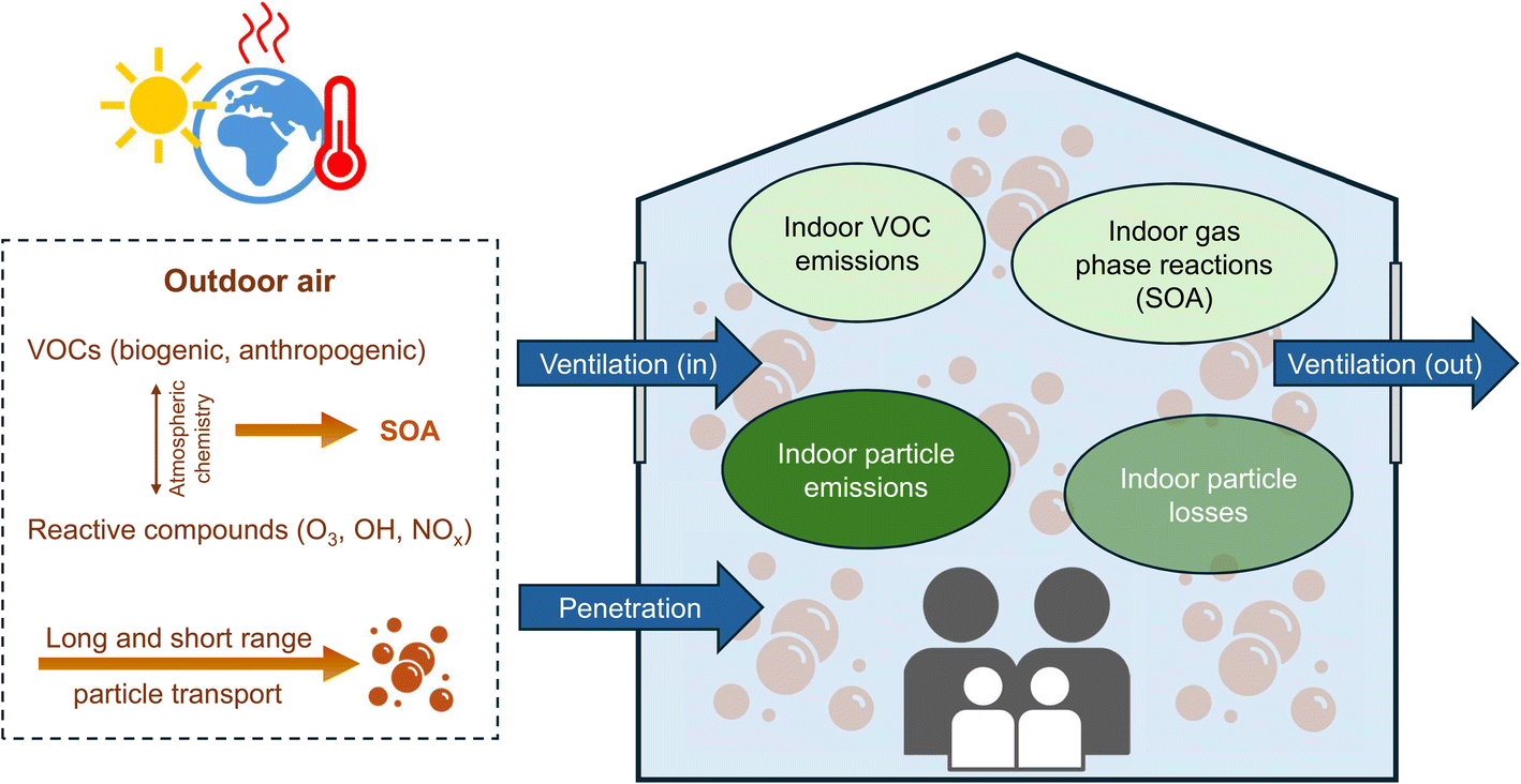Fig. 1 Influences of dynamic and reactive processes outdoors and indoors on the indoor exposure of residents to particles.

In addition, global warming will not only lead to increased indoor discomfort and heat stress, but will also affect temperature-related indoor chemical–physical processes that alter indoor gas and particle concentrations.²⁸ In order to mitigate the impacts of climate change and adapt to the expected environmental conditions, improved building characteristics and changes in occupant behavior will be necessary. Tighter buildings are a consequence, which will allow two main objectives to be achieved: (a) thermal insulation and (b) lower penetration of outdoor pollutants into indoor air. The building adaptation actions may include reinforcement of insulation by implementing new materials and smart building technologies that can control and adjust air exchange and other climatic parameters.^28–31 For example, warmer winters may require longer periods of open windows, while warmer summers may require air conditioning and reduce the duration of open windows.

In this study, we will investigate and discuss the possible changes in indoor airborne particle concentrations as a result of climate change. Both outdoor and indoor sources are considered. The calculations are based on the Indoor Air Quality and Climate Change (IAQCC) model we published earlier³² and the derived developments for temperature and humidity until the year 2100.²⁸ The strength of the model lies in the fact that it combines various influencing factors such as environmental conditions, building parameters, indoor emissions and occupants' activities simultaneously and comprehensively. The simulation of indoor climate and indoor gas-phase reactions has been validated using experimental data, and the model was successfully applied in the prediction of short- and long-term indoor gas-phase reactions under selected future climate and emission scenarios.²⁸ Our methods do not allow for predictions for individual living situations. Rather, they are estimates that become likely in certain climate scenarios, which can be used to better assess future exposure and take preventive measures.

2 Methods

2.1 Model description

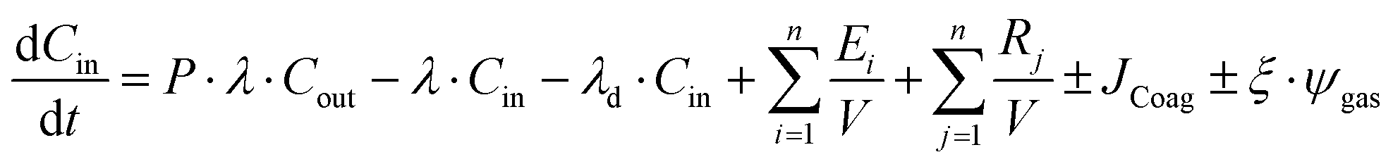
To estimate indoor particle exposure, the IAQCC model accounts for indoor particle emissions from occupant activities, particle transport between indoors and outdoors (including ventilation and penetration), indoor particle loss (including deposition and coagulation), resuspension, and particle formation from gas-phase reactions. It is based on the Indoor Aerosol Model (IAM) developed by Hussein et al.^33,34 The IAQCC model can simulate the temporal development of the particle number size distribution (PNSD) in indoor spaces, which is beneficial for determining the particle size-dependent exposure in the human body.

The general balance equation for simulating indoor particle concentrations can be mathematically described by using eqn (1):

where C_in and C_out are the indoor and outdoor particle concentrations (# cm⁻³ or μg m⁻³). P is the outdoor air penetration factor, which is dimensionless and defined as the proportion of particles in the infiltrating air that passes through the building envelope. λ is the air change rate (h⁻¹), and λ_d is the particle deposition rate on indoor surfaces (h⁻¹). E is the emission rate of source i (# h⁻¹ or μg h⁻¹), and V is the room volume (m³). R is the resuspension rate of source j for coarse particles (# h⁻¹ or μg h⁻¹). J_Coag is the coagulation term for the gain or loss of particles. ψ_gas is the reaction rate due to gas-phase chemistry, and the ξ represents the yield of SOAs. This mass balance eqn (1) is considered for a given particle diameter range (represented by an average diameter D_p), in which the chemical–physical properties are rather similar.

2.2 Test house description

A single-family house located in a rural area in Leipzig, Germany (latN: 51°22′, longE: 12°30′), was selected as the test house. The house had natural ventilation and was inhabited by two residents. In the test house, indoor and outdoor PNSD, PM_2.5 and PM₁₀ data were collected during a measurement campaign in Germany.³⁵ In addition, occupant activities and ventilation data were recorded and estimated. The test house had a total living area of 220 m², and the dimensions of the measured room were length = 4 m, width = 4.5 m, and height = 2.55 m. The room had one double-glazed window (1.8 m²) facing west, and one double-glazed window (5 m²) facing south. In this work, IAQCC simulations were carried out for this room. To estimate gaseous emissions from furniture, an A/V ratio of 3.5 m² m⁻³ was assumed, which lies within the typical range for a furnished home (2.5–3.5 m² m⁻³).^36,37 The total surface area of the room was 160 m². Considering the area of the walls, ceiling and floor (79 m²), the remaining area was assumed to be the furniture area (81 m²).

The house was built in 1995 and is a solid structure with refurbished windows. Details of the building materials and insulation of the house were not documented. To estimate the heat and moisture transfer between the building envelopes of the test house, the data on building materials and heat transfer coefficients (U-values) were applied from the data published by the EU project TABULA (Typology Approach for Building Stock Energy Assessment).³⁸ Based on the existing types of residential buildings and heating systems available in European countries, the TABULA project characterizes the common structures for building typologies and provides typical building data such as thermal envelope areas, structures, and U-values. For single-family homes built between 1995 and 2001, the typical heat transfer coefficient (U-value) is 0.3 W m⁻² K⁻¹ for exterior walls and 1.9 W m⁻² K⁻¹ for windows. The exterior wall complies with the German Thermal Insulation Ordinance for new buildings released in 1994 and valid from 1995 until 2002,³⁹ according to which the required U-value for the exterior wall should be below 0.5 W m⁻² K⁻¹, and the windows should slightly exceed the limit value for renewed windows (U ≤ 1.8 W m⁻² K⁻¹).

2.3 IAQCC model setup and simulation parameters

The IAQCC model consists of five sub-models dealing with building heat and moisture transfer, gas and particle emissions from indoor materials and occupant activities, gas chemical reactions, aerosol particle dynamics, mold growth, occupant comfort and pollutant exposure estimation. Key processes and parameters that are considered in the model simulation for indoor particles are described below.

2.3.1 Ventilation and penetration. Nazaroff^40,41 reviewed residential ventilation rates, which ranged from 0.1 h⁻¹ to 4 h⁻¹, with a typical value of 0.5 h⁻¹. For air exchange rates in European housings, Salthammer⁴² calculated a geometric mean of 0.5 h⁻¹. Zhao et al.³⁵ reported ventilation rates in 40 German households that showed a similar range, with average ventilation rates of 0.2 h⁻¹ and 3.7 h⁻¹ with windows closed and open, respectively. In this study, typical window-opening habits were used to simulate natural ventilation in the test house: in summer (June–August), windows were assumed to be closed during the day (8:00–18:00), open in the evening (18:00–22:00), and tilted at night (22:00–08:00); for the rest of the year, the windows were opened briefly in the morning (07:00) and in the evening (18:00). Air change rates during window opening and tilt opening were assumed to be 4 h⁻¹ and 1 h⁻¹, respectively. During window-closed periods, an infiltration rate of 0.4 h⁻¹ was assumed for the test house. The particle size-dependent penetration factors were taken from the results of real households in Germany published by Zhao et al.,⁴³ where the mean penetration factor is P = 0.6. For mechanical ventilation, the particle size-dependent penetration factors through various filters were considered, using particle size-resolved filtration efficiency data (particle size range 0.1–10 μm) provided by Goodfellow and Tähti⁴⁴ (see ESI,† Section S1). Note that the filter data by Goodfellow and Tähti correspond to the previous standard for testing air filters in Europe EN 779,⁴⁵ which was replaced by the international standard ISO 16890 in 2016.⁴⁶

2.3.2 Emission. The data on particle emission rates are also available in the publication by Zhao et al.,⁴³ where typical indoor activities of real-use German dwellings were taken into account. Additionally, the particle size-resolved emission rate in the same test house was calculated and presented in our earlier work.³² For the long- and short-term simulation of particle dynamics in the test house, to reflect a real-life scenario, daily activity patterns measured on January 17, 2017 were applied, including the particle number emission rate, time, and duration data for the three indoor activities. Details regarding particle measurements are provided in Section 2.2 and in Section S2 of the ESI.†

The gas-phase emission was also considered in order to determine the influence of particle formation due to the gas-phase reaction. Considering the furniture of the test house as wooden furniture, the temperature-dependent emission rate of gas compounds can be calculated as:

E = SER_A·A_fur·f (2)

where SER_A is the area-specific emission rate (μg m⁻² h⁻¹), A_fur is the furniture surface area (m²), and f is the temperature-dependent coefficient (dimensionless). The data of the time-dependent function of SER_A and f were presented in Zhao et al.,²⁸ where the SER_A was derived based on the general emission data available at Fraunhofer WKI, and f was calculated based on literature data. An example of the calculation of the emission rate of limonene from wooden furniture can be found in Section S3 of the ESI.†

Data on possible unit-specific emission rates of indoor gas pollutants are available from the publications of a Europe-wide project EPHECT (Emissions, exposure Patterns and Health Effects of Consumer Products in the EU).^47–49 As information on gaseous pollutants from indoor activities in the test houses was not available, a common source, the air freshener spray, was assumed based on the data provided in the EPHECT project, where the average limonene emission rate is 4453 μg h⁻¹.⁵⁰

2.3.3 Resuspension. Indoor resuspension was taken into account when calculating the mass concentration of fine and coarse particles (PM_2.5 and PM₁₀). Under real-life conditions, indoor resuspension is usually caused by residents' movements, e.g. walking.⁵¹ Since there were no records of resident “walking times” during the measurements, the resuspension period in the simulation was assumed to be the time when the PM₁₀ concentration showed a peak. The resuspension rate can be calculated as:

R = l_a·r_a·A_floor (3)

where the floor loadings (l_a) and resuspension rate coefficient (r_a) data are taken from Bramwell et al.⁵² for various floorings and conditions, A_floor is the floor area (m²). The carpet in the test house was assumed to be “medium” loaded, with a corresponding l_a of 50 mg m⁻² and 130 mg m⁻² for PM_2.5 and PM_10–2.5, and r_a of 9.4 s⁻¹ and 87.5 s⁻¹, respectively.

2.3.4 Deposition. Deposition of particles on indoor surfaces can be influenced by the furnishing type, area and airflow conditions.⁵³ The deposition rate also varies for different particle size ranges. The deposition loss of indoor particles considers deposition onto indoor horizontal surfaces and vertical surfaces (i.e., ceiling, ground, walls, and furniture). For a specific surface i, the deposition rate λ_d can be calculated as:where v_d,i (m s⁻¹) is the deposition velocity of aerosol particles onto the indoor surface i, which has the surface area A_i. The particle size-resolved deposition velocity was computed using the approach of Lai and Nazaroff⁵⁴ and Seinfeld and Pandis,⁵⁵ taking into account gravitational settling, Brownian diffusion and eddy diffusion, with the estimated friction velocity near indoor surfaces, particle diameter and temperature as inputs.

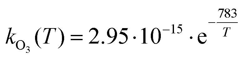
The deposition of ozone and OH indoors was also considered, with the deposition velocity data for ozone (0.036 cm s⁻¹) and OH (0.007 cm s⁻¹) taken from Sarwar et al.⁵⁶

2.3.5 Coagulation. Based on the IAM model, the IAQCC extended the coagulation simulation by including particle formation. The PNSD changes during each simulation time step while maintaining overall mass balance, i.e., the mass lost by small particles due to collisions is equal to the mass gained by the corresponding large particles. J_Coag between particles in the neighbor size ranges D_pi and D_pi+1 can be calculated as:

J_Coag = K·C_in,Dpi·C_in,Dpi+1 (5)

where C_in,Dpi and C_in,Dpi+1 are the particle number concentration of the particles in the corresponding size ranges. The coagulation coefficient K was computed based on Fuchs theory in the transition region and in the free molecule region, assuming that all collisions lead to coagulation of the two colliding particles, with particle diameter and temperature as inputs.⁵⁵ The PNSD was set for 12 particle size fractions (10–800 nm), which allows for better capture of coagulation loss and formation processes.

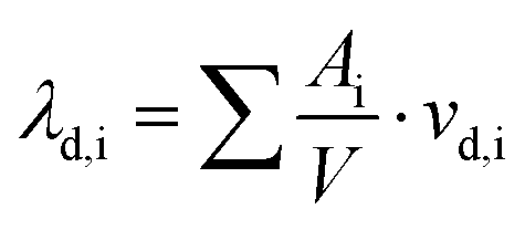
In order to quantify the influence of climate change, the fundamental parameters in the deposition and coagulation model were introduced as a function of temperature instead of a constant value, including dynamic viscosity (μ), air density (ρ), and air mean free path (λ_air). The relevant equations for calculating particle deposition and coagulation are given in the ESI† (Section S4). Consequently, temperature changes due to climate change are reflected in these two processes, thus affecting the overall indoor particle concentrations.

2.3.6 Gas reaction. The reaction rate of gas-phase chemistry was calculated as:

ψ_gas = k_[gas][ox]·C_gas·C_ox (6)

where k_[gas][ox] is the bimolecular reaction rate constant for the organic gas compound and oxidant (ox), and C_gas and C_ox are the concentrations of the organic gas and oxidant, respectively. As a common indoor gas substance, limonene was selected as an example for simulating the reaction with ozone and OH radicals. The reaction products are based on the initial reactions with ozone and OH radicals according to the Master Chemical Mechanism (MCM, v3.3.1).⁵⁷ OH production from limonene and ozone reaction was also taken into account with an OH yield of 0.86.⁵⁶ The temperature-dependent gas-phase reaction constant (cm³ molecule per s) with ozone and OH radicals, k_O3 and k_OH, can be described using eqn (7) and (8),⁵⁸where T is the temperature (K). Based on the work of Saathoff et al.,⁵⁹ a value of ξ = 0.5 was chosen as the SOA yield for the limonene/ozone system.

2.4 Model validation

As validation, simulations were carried out for the above-described measured room in the test house. The outdoor PNSD and occupants’ activity data were illustrated in our earlier work in Salthammer et al. (2022).³² Assuming that the initial indoor PNSD is zero, the number of particles transported from outdoors can be calculated using the measured outdoor PNSD and eqn (9):

Emission data from three indoor activities measured on January 17, 2017 – toasting (07:00), baking (14:00) and frying (19:00) – were used for the simulation. The particle size-resolved emission rates of these three activities are listed in Table S2 of the ESI.† The indoor PNSD was then calculated using eqn (1) taking into account particles transported from outdoors, emitted indoors, and lost indoors. The results of the simulated PNSD and PNC show good agreement with the measured values (see Fig. S2 and S3 in the ESI†), with a coefficient of determination (R²) of 0.96 for the linear correlation of simulated and measured PNC.

For the simulation of indoor PM_2.5, and PM₁₀ due to resuspension, the carpet in this house was assumed to be “medium” loaded. In addition, the contribution of toasting, baking and frying activities indoors was taken into account by adding the PM₁ concentration calculated from the PNC.

The measured and simulated results show a comparatively poor correlation, with an R² of 0.25, 0.66, and 0.43 for PM₁, PM_2.5, and PM₁₀, respectively. However, the simulated peak times match the measured values (see Fig. S4 in the ESI†), and the mean values are at the same level as the measured ones: the measured mean concentrations of PM₁, PM_2.5, and PM₁₀ are 6.1, 9.6, and 26.2 (μg m⁻³), respectively, and the simulated values are 4.7 μg m⁻³, 9.6 μg m⁻³, and 19.7 μg m⁻³, respectively. Considering that the resuspension source of PM_2.5, and PM₁₀ includes only “walking” based on literature data, and that many unknown activities or parameters can occur under real conditions, the results are within an acceptable range.

2.5 Future climate

2.5.1 IPCC scenarios. The gas and particle concentrations in air can be influenced by changing meteorological conditions, such as temperature, precipitation, wind speed, and atmospheric stability. At the same time, the extent of climate change and emissions over the next century will depend on the clean air legislation that is implemented. The IPCC Sixth Assessment Report deals with the climate response to five illustrative future climate scenarios, the Shared Socio-economic Pathway (SSP) scenarios, ranging from low to high greenhouse gas emission assumptions.¹ In this report, it is predicted that the long-term (2081–2100) change in global surface temperature compared to the present (baseline period 1995–2014) is very likely to be between +0.2 °C and +4.9 °C. In line with our assessment of the impact of climate change on indoor gas chemistry in Zhao et al.,²⁸ the SSP1-2.6, SSP2-4.5 and SSP5-8.5 scenarios were selected, corresponding to low, medium and very high greenhouse gas emissions, respectively.

The initial weather data for the test house area (Leipzig) were taken from the Test Reference Year (TRY) data published by Deutscher Wetterdienst (DWD; reference coordinates 51,3731° N, 12,5063° O, access date 2024.07.26).⁶⁰ TRY datasets represent the typical weather pattern of the corresponding area (hourly data for a full year with a spatial resolution of 1 km²). The data were created on the basis of a statistical analysis of real measured weather data for the period 1995–2012, which is in a similar range to the selected baseline period in the SSP scenarios (1995–2014).⁶¹ The long-term simulation (see Section 3.1) started with 2020, which already considered the temperature difference compared to the baseline value.

The interactive IPCC WGI Atlas provides model projection data for future global and regional surface temperatures, precipitation as well as concentrations of air pollutants such as ozone and PM_2.5.^62,63 For Western and Central Europe it predicts a declining trend in PM_2.5 levels for all three scenarios. By 2100, the annual mean mass concentration of PM_2.5 will decrease by 3.5, 3 and 2 μg m⁻³ for the SSP1-2.6, SSP2-4.5 and SSP5-8.5 scenarios, respectively. Since the predictions for PM₁₀ and PNC are not available in the IPCC Atlas, for simplicity they are assumed to follow the same trend as PM_2.5, using the same change factor.

The initial data for the particle mass concentrations of outdoor PM₁₀ and PM_2.5 in rural areas were taken from historical data measured in Germany (average of all stations with available data) from the database published by the European Environment Agency.⁶⁴ To assess the impact of using the daily mean or annual mean values of outdoor PM₁₀ and PM_2.5 concentrations as input variables on the indoor simulation results, a case study was conducted for one year (ESI S5†). The results show that the effects of changes in daily outdoor PM₁₀ and PM_2.5 concentrations on simulated indoor annual mean concentrations can be neglected.

The initial PNSD data (detailed data see ESI,† Section S6.1) were based on the rural background mean values measured and published by the German Ultrafine Aerosol Network (GUAN),^65,66 which have been measured continuously since 2009 at 17 atmospheric observatories in Germany. The PNC was calculated by integrating the PNSD over the specified particle diameter range.

Hourly data on the diurnal variation of outdoor ozone and OH radicals were used in the model simulation, based on Melkonyan and Kuttler⁶⁷ and Emmerson et al., respectively.⁶⁸ The details of initial data on outdoor ozone and OH radicals, as well as future prediction of ozone concentrations for the three SSP scenarios (including the increasing and decreasing trend) were also discussed in Zhao et al.²⁸

The annual mean values of these air pollutants are summarized in Table 1.

Table 1 Annual mean ozone and particle mass and number concentrations in 2020 (based on historical data measured in Germany) and 2100 under selected scenarios (based on IPCC projections) applied in the long-term simulations

Pollutant	Annual mean outdoor concentration
	2020	2100 under SSP5-8.5	2100 under SSP2-4.5	2100 under SSP1-2.6
PM10 (μg m^−3)	16	14	13	12.5
PM2.5 (μg m^−3)	10	8	7	6.5
PNC (# cm^−3)	4312	3080	2464	2156
Ozone (μg m^−3)	56	62	50	34

---

2.5.2 Extreme weather conditions. Two types of extreme weather conditions were considered in this work. The first is extreme heat periods (heatwaves) accompanied by high ambient ozone, and the second is dust storm events.

Extreme heat periods (including heatwaves) have become more frequent and more intense in most land regions since the 1950s.¹ Several studies reported elevated ozone concentrations during heatwaves.^18,69–73 The European Environment Agency (EEA) provides a comprehensive database with current concentrations and trends for climatic parameters and pollutants⁷⁴ (note that the latest report is for 2022; current data can be found on the EEA website https://www.eea.europa.eu/en). Ozone episodes occur regularly in Germany during the summer months, with a clear increase in the southern part. Fig. 2 shows a typical daily episode (hourly averages) for the urban traffic station and urban background station in Leipzig. On this day, the maximum temperature in the Leipzig area was 33.7 °C. The ozone data from the DESN059 urban background station were used as a basis for further calculations.

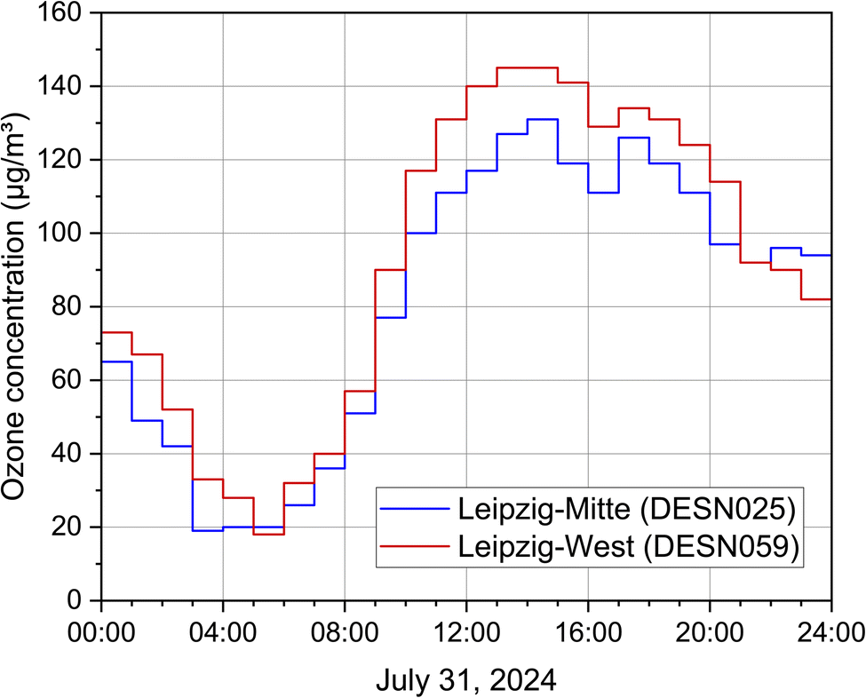Fig. 2 Outdoor ozone concentrations (hourly averages) on a heatwave day in Leipzig, Germany. The data for station DESN025 (Leipzig-Mitte, urban traffic) and DESN059 (Leipzig-West, urban background) were taken from the online database of the German Environment Agency (UBA, https://www.umweltbundesamt.de/en/data).

It is well-known that aerosols and their components can travel intercontinental distances in the atmosphere.⁷⁵ Deserts in particular represent geochemical reservoirs that have a lasting impact on the climate. For example, the air quality in Beijing especially in spring is affected by sandstorms from the Gobi Desert,⁷⁶ and the Canary Islands often suffer from Saharan dust events caused by the aforementioned Calima.²⁰ Sahara dust events are not unknown in Europe, but have so far mainly occurred in the southern part of the continent. For some time now, however, Central Europe has also been hit more frequently by such events,⁷⁷ one cause being the interplay of the Scirocco and Foehn winds. This leads to unusually high particle concentrations in outdoor air, e.g. in 2024 around the end of spring in the Leipzig area, as shown in Fig. 3. It is clear that PM_2.5 and PM₁₀ concentrations in the range of 100–150 μg m⁻³ have a massive impact on indoor air quality, so such events must be taken into account in exposure modeling.

Fig. 3 Outdoor PM_2.5 and PM₁₀ concentrations (hourly averages) from March 29 to April 3, 2024 in Leipzig, Germany. The data for station DESN059 (Leipzig-West, urban background) were taken from the online database of the German Environment Agency (UBA, https://www.umweltbundesamt.de/en/data).

3 Results and discussion

3.1 Long-term prediction of indoor particle exposure (IPCC scenarios)

Long-term simulations (2020 to 2100) of indoor climate and particle concentrations were performed for the test houses under three IPCC climate scenarios: SSP1-2.6, SSP2-4.5, and SSP5-8.5. By 2100, the annual mean outdoor temperature would have increased by 0.8 °C, 2.2 °C, and 5.5 °C starting from 10.5 °C in 2020 according to the three climate scenarios, respectively. The simulated indoor temperature increased correspondingly (from 19.1 °C) by 0.4 °C, 1.1 °C, and 2.8 °C, respectively. The increasing temperature directly influences the emission rate of limonene from indoor wooden furniture and the reaction rate of the gaseous substances.

Fig. 4 shows the annual mean concentrations of ozone, OH radicals, limonene, and the produced SOA for this reaction system. The simulation of indoor ozone considers outdoor transport, indoor deposition loss and reaction loss with limonene, which can be calculated using eqn (1). Indoor ozone concentrations follow the same increasing or decreasing trend as the outdoor ones under the various future scenarios. As a product of the ozone/limonene reaction, OH radical concentration is in the range of 0.5–1.0 × 10⁵ molecules cm⁻³ up to 2100. The review article by Gligorovski et al.⁷⁸ summarizes typical indoor OH for simulating the gas-phase reaction of ozone with alkenes (e.g., limonene) and indicates a concentration range between 10⁴ and 10⁵ molecules cm⁻³. The OH radical concentrations modeled in this work are within this typical range.

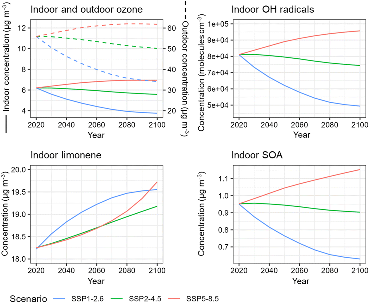Fig. 4 Annual average outdoor ozone concentration predicted by three SSP climate scenarios, and the simulated indoor concentrations of ozone, OH radical, limonene, and SOA in the test house from 2020 to 2100 under the corresponding scenarios.

The sources of limonene in the test house include the daily short-term use of air freshener sprays and temperature-dependent emissions from indoor furniture. Limonene reacts with both ozone and OH radicals. Note that other indoor reaction pathways, such as the photochemical formation of OH radicals indoors involving nitrous acid (HONO) and NO_x, were not considered in this simulation. However, despite the increasing or decreasing future trend in ozone and OH radical concentrations, indoor limonene concentrations show an increasing trend for all three SSP climate scenarios. This can be attributed to the high temperature-dependent limonene emissions from indoor furniture. As shown in Fig. 5, for the 81 m² wooden furniture in the test house, the limonene emission rate increases by 19.2 μg h⁻¹ per degree increase in temperature. Fig. 5 also shows the temperature-dependent loss rate of limonene (μg h⁻¹) due to reactions with ozone and OH radicals, calculated by using the gas-phase reaction rate (ψ_gas in μg m⁻³ h⁻¹) × room volume (V = 46 m³). According to eqn (7) and (8), the temperature-dependent reaction constants k_O3 and k_OH show an exponential increase and decrease, respectively. Considering a typical indoor concentration of ozone (3 ppb ≈ 6 μg m⁻³ at p = 1013 hPa, T = 298 K),⁷⁹ limonene (4 ppb ≈ 22 μg m⁻³ at p = 1013 hPa, T = 298 K) and OH radical concentration (1 × 10⁵ molecules per cm),³⁶ the temperature-dependent limonene loss rate due to reaction with ozone is much lower than the furniture emission rate in the test house. Consequently, SOA formation from the limonene/ozone reaction systems in the test house is expected to decrease under the SSP1-2.6 and SSP2-4.5 scenarios and increase for the SSP5-8.5 scenario (see Fig. 4).

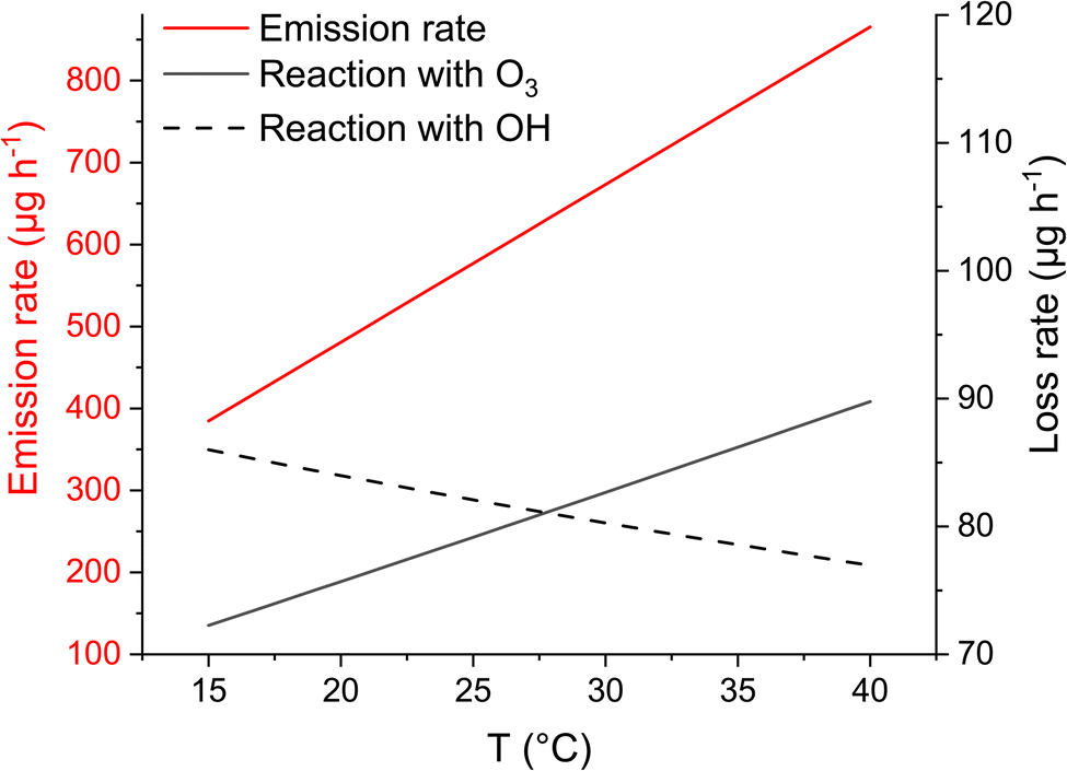Fig. 5 Temperature-dependent limonene emission rate from wooden furniture (81 m²) in the test house (room volume 46 m³), and loss rate due to reaction with ozone (6 μg m⁻³) and OH radicals (1 × 10⁵ molecules per cm) at a limonene concentration of 22 μg m⁻³.

The IPCC predicts decreasing future trends in global surface particle concentrations as a result of air pollution legislation that has been or is expected to be implemented (Table 1). This means that the amount of particles transported from outdoors to indoors will also be reduced. Although indoor SOA formation will increase under the SSP5-8.5 scenario, the simulated total indoor particle mass and number concentrations in the test house will decrease for all scenarios (see Table 2). This indicates that the change in outdoor particle concentrations has a greater impact on future indoor particle concentrations. Note that the indoor particle emissions from residential activities (e.g., baking, roasting, and frying) were assumed to be constant on a daily basis. For SOA formed via gas-phase reactions, even in the worst-case SSP scenario (SSP5-8.5), it is only a small fraction of future particle mass concentrations of PM_2.5 or PM₁₀.

Table 2 Simulated annual mean indoor particle mass and number concentrations in 2020 and 2100 under three SSP scenarios

Pollutant	Annual mean indoor concentration
	2020	2100 under SSP5-8.5	2100 under SSP2-4.5	2100 under SSP1-2.6
PM10 (μg m^−3)	8.8	8.2	7.6	7.1
PM2.5 (μg m^−3)	6.7	6.1	5.5	5.0
PNC (# cm^−3)	8988	8767	8202	8070

---

According to the WHO Global Air Quality Guidelines,⁸ the annual PM₁₀ and PM_2.5 air quality guideline (AQG) levels are 15 μg m⁻³ and 5 μg m⁻³, respectively. Based on the assumptions made for the test houses, the annual mean indoor PM₁₀ concentration appears to be below the guideline requirements (Table 2). As for PM_2.5, it will meet the guideline values in 2100 under the SSP1-2.6 scenario and will be slightly above the guideline requirements under the remaining scenarios. Note again that in this work, only limited sources of indoor PM₁₀ and PM_2.5 were considered (see Section 2.3). The simulated concentrations of PM₁₀ and PM_2.5 are lower than experimental data from a typical German household presented by Zhao et al. (25 μg m⁻³ and 13 μg m⁻³, respectively).³⁵

Since the goal of this work is to estimate the magnitude of the produced particle mass, SOA formation is not considered in the PNC and PNSD simulations at this stage. Nevertheless, indoor SOA formation can significantly increase the number concentration of fine and ultrafine size particles, which contribute comparatively less to the mass concentration due to their small size.^80–82

Fig. 6 shows the influence of temperature changes on the deposition rate for different particle sizes (10–800 nm) on indoor surfaces. The maximum deposition rate is shown at the smallest size and the minimum deposition rate is shown in the 100–200 nm particle size range (Fig. 6a). The simulated annual mean indoor PNSD for 2020 and 2100 can be found in ESI,† Section S6.2. By multiplying the annual mean PNSD in the test house, the number of lost particles in each size range shows a different pattern (see Fig. 6b), where the highest particle number loss is shown in the 12–40 nm size range. Overall, the particle deposition losses decrease with increasing temperature. However, the influence of temperature on particle deposition losses is relatively small compared to the deposition rates and number concentrations for different particle sizes.

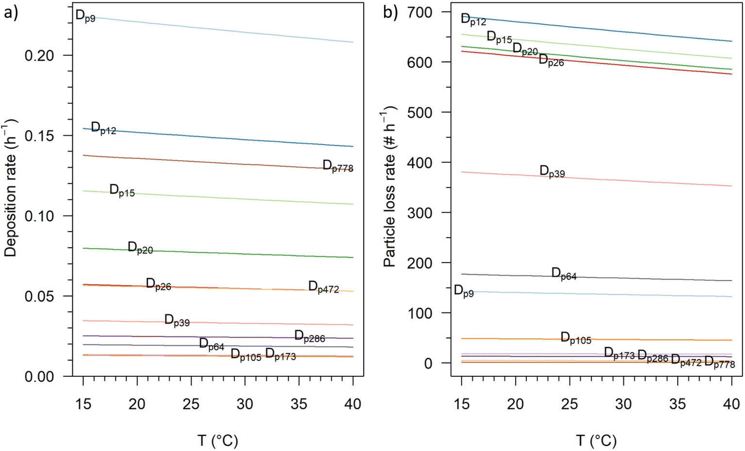Fig. 6 Temperature-dependent (a) particle deposition rate (h⁻¹) and (b) number of particles lost due to deposition on indoor surfaces (# h⁻¹) for 12 particle size ranges (10–800 nm).

3.2 Indoor particle exposure during extreme weather

Indoor climate and particle concentrations were simulated for the test houses under the two extreme weather conditions, i.e. an ozone episode during a heatwave, and dust storm episode. For the case of the ozone episode, the IAQCC model simulation provided insight into the exposure levels of indoor ozone, limonene, and the formed SOA. For the dust storm episode, the focus is on the elevated concentration of PM_2.5 and PM₁₀ indoors.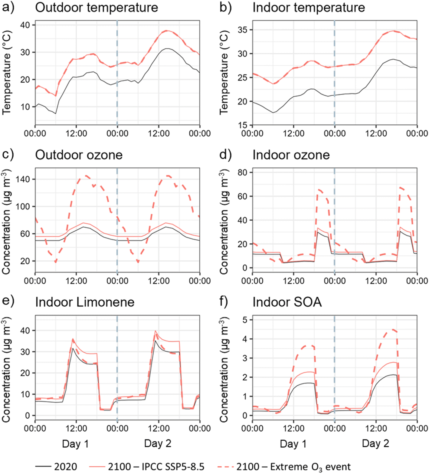

3.2.1 High ozone episode during a heatwave. To investigate the effects of extreme ozone events on indoor air during heat waves, two summer days in 2020 were compared with a hypothetical scenario in 2100 (see Fig. 7). In 2020, the daily maximum ambient temperature suddenly rose from about 23 °C on day 1 to about 31 °C on day 2. According to IPCC scenario SSP5-8.5, the summer temperature is expected to rise by around 7 °C by 2100. Under the assumed indoor condition of the test house, in 2020, the daily maximum indoor air temperatures are 23 °C on day 1 and 28 °C on day 2, respectively. Under IPCC Scenario SSP5-8.5, in 2100 the projected maximum daily temperatures are 27 °C on day 1 and 35 °C on day 2, respectively.

Fig. 7 Simulated indoor temperature, ozone, limonene and SOA concentrations for two summer days in 2020 (black), 2100 under the SSP5-8.5 scenario (red), and 2100 during a extreme ozone event (red dashed): (a) outdoor temperature, (b) indoor temperature, (c) outdoor ozone, (d) indoor ozone, (e) indoor limonene, (f) indoor SOA. Note that the data from Fig. 2 were used to simulate the 2100 extreme ozone event.

The heatwave condition might be accompanied by extreme ozone concentration variation. Under normal conditions in 2020, the ambient ozone concentration varies daily between 50 μg m⁻³ and 70 μg m⁻³ (Fig. 7c). According to the IPCC SSP5-8.5 scenario, the mean outdoor ozone concentration will increase by 6 μg m⁻³ from 2020 to 2100 (Table 1). Considering the extreme ozone concentration variation according to Fig. 2, the ambient ozone concentration in 2100 would vary daily between 18 μg m⁻³ and 145 μg m⁻³.

The corresponding indoor ozone concentration was simulated considering the summer ventilation variations assumed in the IAQCC model simulation, as described in Section 2.3: windows closed from 08:00 to 18:00 (low ventilation rate of 0.4 h⁻¹), windows opened from 18:00 to 22:00 (high ventilation rate of 4 h⁻¹), and windows tilted overnight from 22:00 to 08:00 (ventilation rate of 1 h⁻¹). Under high ventilation conditions, the ambient ozone entered the indoor air efficiently. Therefore, even when no extreme ozone events occur, the maximum indoor ozone concentration in 2020 and 2100 reaches about 30 μg m⁻³ (Fig. 7d). During extreme ozone events, the maximum indoor ozone concentration can reach up to about 70 μg m⁻³ when the windows are open. This value is below the WHO's short-term AQG level for ozone, where the average daily maximum 8 hour mean value is 100 μg m⁻³.⁸ Nevertheless, given that extreme ozone events during heatwaves will occur more frequently in the future, such high indoor ozone concentrations are likely to exceed the peak season AQG level of 60 μg m⁻³ (peak season: the six consecutive months of the year with the highest six-month running-average ozone concentration).

The high concentrations of indoor ozone affected the concentrations of indoor limonene and SOA. As mentioned in Section 3.1, the sources of indoor limonene are the air freshener and temperature-dependent furniture emissions. The indoor limonene concentration is generally higher on day 2 than on day 1, which is due to the higher temperature on day 2 (Fig. 7e). For the two cases in 2100 shown in Fig. 7 (i.e. for the SSP5-8.5 scenario and the extreme ozone episodes), the amount of limonene emitted indoors is the same because the temperature profiles are the same. During extreme ozone events, indoor limonene concentrations are therefore lower because more limonene reacts with elevated ozone. This leads to the formation of SOAs during extreme ozone events being more than 60% higher than in the SSP5-8.5 scenario and more than twice as high as in 2020 (Fig. 7f).

3.2.2 Dust storm events. During dust events, the ambient particle concentrations are significantly elevated. As a model case, the effects of Sahara dust on indoor PM₁₀ and PM_2.5 concentrations were studied using data from Leipzig from March 29 to April 3, 2024 as presented in Fig. 3. During this dust event, outdoor PM₁₀ and PM_2.5 concentrations increased dramatically from March 30 and reached a maximum on March 31 at 145 μg m⁻³ and 120 μg m⁻³, respectively (Fig. 8a and b). These concentrations are significantly higher than the annual average concentrations in 2020. As already outlined in Section 2.4.1, the initial data for outdoor PM₁₀ and PM_2.5 particle mass concentrations are average concentrations in rural areas measured in Germany, i.e. the monitoring stations were less influenced by regional pollution such as urban traffic. Based on the IPCC SSP5-8.5 scenario, the annual mean outdoor PM₁₀ and PM_2.5 concentrations would both decrease by 2 μg m⁻³ from 2020 to 2100 (Table 1). For indoor particle simulation for 2020 and 2100 under the SSP5-8.5 scenario, the annual mean outdoor PM₁₀ and PM_2.5 particle mass concentrations were applied, and thus their daily variations cannot be seen in Fig. 8a and b.

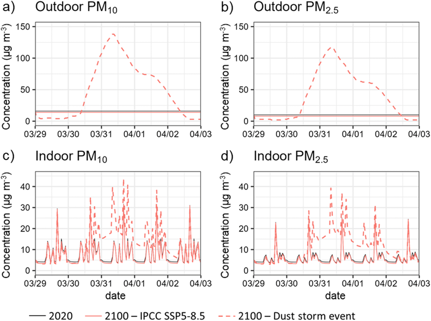Fig. 8 Simulated indoor concentrations of PM₁₀ and PM_2.5 for a five-day period in 2020 (black), 2100 under the SSP5-8.5 scenario (red), and 2100 during a dust storm event (red dashed): (a) outdoor PM₁₀, (b) outdoor PM_2.5, (c) indoor PM₁₀, (d) indoor PM_2.5. Note that the data from Fig. 3 were used to simulate the 2100 dust storm event.

The simulated indoor PM₁₀ and PM_2.5 concentrations show clear peaks and daily variations (Fig. 8c and d), which can be attributed to the indoor activities of residents as described in Section 2.3. Note that this dust event is not in the summer months, so unlike the ventilation profile during the heatwaves, the windows here are only assumed to be opened briefly at 07:00 and 18:00 (Section 2.3). In 2020, peak indoor PM₁₀ and PM_2.5 concentrations occurred at around 14:00 daily and are about 30 μg m⁻³ and 25 μg m⁻³, respectively. The highest calculated indoor PM₁₀ and PM_2.5 concentrations during the dust event appeared on March 31 with 45 μg m⁻³ and 40 μg m⁻³, respectively. In addition, a significant increase in peak concentrations can be predicted for 07:00 and 18:00 when windows are open, with the PM_2.5 concentration at 07:00 on March 31 even exceeding the peak at 14:00 caused by residential activity.

WHO Air Quality Guidelines also define the short-term AQG levels for PM₁₀ and PM_2.5, where the 24-hour average guideline values are 45 μg m⁻³ and 15 μg m⁻³, respectively.⁸ During this dust storm, the simulated 24 hour average indoor PM₁₀ concentrations are all below the guideline value, with the highest concentration of 22 μg m⁻³ on March 31. However, the 24 hour average indoor PM_2.5 concentration reached 20 μg m⁻³ on March 31, exceeding the guideline value.

These two examples of extreme weather events clearly show that suddenly increased concentrations of ambient pollutants can also lead to high levels of acute indoor exposure. Consequently, technical measures, official warnings and recommendations on appropriate living behavior are needed to better protect residents under such conditions.

3.2.3 Future ventilation techniques and strategies. The question of how private and public buildings should be ventilated in the future has been an intensively discussed topic since the SARS-CoV-2 pandemic.⁸³ This study has shown that providing clean air indoors will become more relevant but also more difficult in the future. It is important not only to remove pathogens and other pollutants through ventilation, or to deactivate and filter them out using recirculation processes, but also to prevent outside air pollutants entering indoors by ventilation.

The practical problems are obvious. Under extreme weather conditions such as ozone and Sahara dust episodes, it is advisable to keep windows and doors closed. This is only possible for a limited period of time with manual ventilation, as the air exchange rates in well-insulated buildings are usually rather low.⁴⁰ In addition, the water absorption capacity of air increases with temperature, which also increases the risk of mold formation. Consequently, there is a clear trend towards mechanical ventilation in private and public buildings, which has been standard in office buildings for many years. The need for sufficient and continuous clean air delivery in rooms with a high density of people such as schools,⁸⁴ retirement homes⁸⁵ and event arenas⁸⁶ is immediately apparent.

The increasingly noticeable effects of climate change will most likely accelerate the transition to mechanical ventilation, preferably in conjunction with the energy management of the building. This would also consider the demands of heat action plans.⁸⁷ In residential buildings, this idea is being realized with smart homes.²⁹ The necessary sensors are constantly being improved and the smart home concept can in principle be transferred to other building types. Morawska et al.⁸⁸ stated that only a few parameters such as clean air supply, carbon monoxide (CO), carbon dioxide (CO₂) and PM_2.5 are required to assess indoor air quality and control systems.

Almost all mechanical ventilation systems work with a certain proportion of recirculated air. Therefore, cleaning modules in the system are indispensable. For particles, filter technology is standard and its efficiency is now assessed according to ISO 16890.⁴⁶ The minimum requirement for PM₁ is 50% separation efficiency, which corresponds to an F7 filter according to the withdrawn EN 779.⁴⁵ The various particle filter classes as well as similarities and differences between ISO 16890 and EN 779 are discussed by Yit et al.⁸⁹ Regardless of the nomenclature, the filters available today offer effective protection against airborne fine dust.

3.3 Sensitivity analyses

The sensitivity of the simulated indoor particle and gas concentrations to the input parameters is evaluated. The results for the year 2100 under IPCC scenario SSP5-8.5 were used as the “base case”, and selected key input parameters are shown in Table 3, including the outdoor temperature, ventilation rate, and outdoor PM₁₀ and PM_2.5 concentrations, as well as indoor limonene and outdoor ozone concentrations.

Table 3 Sensitivity test for indoor particle and gas concentrations in 2100 under different scenarios of input parameters

Input	Simulated indoor mass concentrations (μg m^−3)
	PM2.5	PM10	O3	Limonene	SOA
Base case (SSP5-8.5)	6.1	8.2	6.9	19.7	1.2
Outdoor only T change	6.9	9.0	6.3	20.0	1.1
Outdoor PM2.5 × 2	7.8	9.9	6.9	19.7	1.2
Outdoor PM10 × 2	6.1	8.6	6.9	19.7	1.2
Ventilation rate 0.2 h^−1	7.0	9.1	2.5	51.7	2.9
Ventilation rate 1 h^−1	6.9	9.1	11.0	10.5	0.4
Ventilation rate 4 h^−1	7.7	10.5	28.8	2.8	0.1
Indoor limonene × 2	6.2	8.3	6.9	21.3	1.3
Outdoor O3 × 2	7.0	9.1	13.9	17.0	2.0
2020	6.7	8.8	6.2	18.2	1.0

---

3.3.1 Change in outdoor temperature. As described in Section 2.5.1, the simulation for the IPCC SSP5-8.5 scenario considered the increase in outdoor temperature and changes in outdoor pollutant concentrations (i.e. decrease in particle concentration and increase in ozone concentration). Another simulation was carried out for only changing the outside temperature under the SSP5-8.5 scenario. Compared to the initial state in 2020, the simulated indoor PM₁₀, PM_2.5 and O₃ concentrations only changed by less than 1% (see Table 3). This suggests that changes in outdoor temperature will only have a minor effect on future concentrations of these indoor pollutants.

3.3.2 Change in outdoor PM₁₀ and PM_2.5 concentrations. Increased outdoor PM_2.5 and PM₁₀ concentrations directly led to an increase in indoor PM_2.5 and PM₁₀ concentrations. Note that when the outdoor PM_2.5 concentration increases, a corresponding increase is also seen in the PM₁₀ concentration. Therefore, the increased outdoor PM_2.5 concentration leads to an increase in both indoor PM_2.5 and PM₁₀ concentrations, while the increased outdoor PM₁₀ concentration only leads to an increase in the indoor PM₁₀ concentration (no increase in PM_2.5 concentration).

3.3.3 Change in the ventilation rate. The base case (SSP5-8.5 scenario) considered a diurnal ventilation profile as described in Section 2.3. For comparison, simulations were conducted again with constant low (0.2 h⁻¹), medium (1 h⁻¹), and high (4 h⁻¹) ventilation rates. The results show that changing the ventilation rate can significantly alter the simulated indoor pollutant concentrations. At low ventilation rates, the amount of outdoor ozone transported indoors is greatly reduced, and so is the amount of indoor limonene transported outdoors, resulting in simulated indoor ozone concentration being extremely low (2.5 μg m⁻³) and limonene concentration being extremely high (51.7 μg m⁻³). At the same time, the formed SOA reaches up to 2.9 μg m⁻³. At medium and high ventilation rates, indoor ozone concentrations increased significantly, while limonene and SOA concentrations decreased significantly. Nevertheless, indoor PM₁₀ and PM_2.5 are still much higher than the base case due to direct outdoor transmission.

3.3.4 Change in indoor limonene and outdoor ozone. Note that the limonene change here refers to the air freshener emission rate becoming twice as high. In both cases, increased concentrations of gas-phase pollutants lead to increased SOA formation, which leads to increased indoor PM₁₀ and PM_2.5 concentrations.

4 Conclusion

It was already stated in the Introduction that climate change can no longer be stopped or avoided. Now, the goal of limiting climate change is also becoming increasingly out of reach. According to the United Nations,⁹⁰ global greenhouse gas emissions reached new highs in 2023. If no further ambition is shown, the best our planet could expect to achieve is global warming of up to 2.6 °C over the course of the century. Society must therefore get ready for a medium to pessimistic scenario, which means SSP2-4.5 or higher. The logical consequence is a two-track catalog of approaches. Of course, the limitation of greenhouse gas emissions must be pursued by all means. At the same time, infrastructure and society should be prepared for the coming decades. This includes improved structural concepts, the retrofitting of existing buildings and new ventilation concepts in order to effectively protect people from heat, cold, rain and wind. Residents will also have to adapt their daily routines to new technologies and necessary requirements.

The IAQCC model³² is a helpful tool for better assessing future impacts of climate change on the personal living environment and can contribute to the development of appropriate action plans. The results of simulations presented in this study allow a reasonable estimate of indoor particle concentrations in the Leipzig area up to the year 2100. However, it must be emphasized again that these are predictions from which obvious trends can be derived, but which do not allow general conclusions to be drawn for individual and specific living situations. By taking into account extreme ozone and particle concentrations in outdoor air and previous studies on heat stress and mold,²⁸ it becomes clear that the current structural substance of buildings in Central Europe hardly meets future requirements. The results also suggest that in many regions of the world with far more extreme weather phenomena and significantly higher pollutant levels,^5,91 the situation is becoming or already is dramatically worse. The negative effects of heat⁸⁷ and air pollutants⁸ on health and quality of life are known and the direction is evident. It is therefore urgently recommended that local authorities also focus on the occupied indoor spaces. This affects not only the private and office sectors, but also schools, retirement homes and hospitals, as the vulnerable part of society needs special protection.

Data availability

Data for this article are available on request from the authors. Please contact Dr Jiangyue Zhao, Fraunhofer WKI, 38108 Braunschweig, Germany. Email: E-mail: jiangyue.zhao@wki.fraunhofer.de.

Conflicts of interest

There are no conflicts to declare.

References

1. IPCC, Climate Change 2021: The Physical Science Basis, Cambridge University Press, Cambridge, UK, 2021.
2. K. L. Ebi, A. Capon, P. Berry, C. Broderick, R. de Dear, G. Havenith, Y. Honda, R. S. Kovats, W. Ma, A. Malik, N. B. Morris, L. Nybo, S. I. Seneviratne, J. Vanos and O. Jay, Hot weather and heat extremes: health risks, Lancet, 2021, 398, 698–708,  DOI:10.1016/S0140-6736(21)01208-3.
3. C. Wasko, R. Nathan, L. Stein and D. O'Shea, Evidence of shorter more extreme rainfalls and increased flood variability under climate change, J. Hydrol., 2021, 603, 126994,  DOI:10.1016/j.jhydrol.2021.126994.
4. S. Clayton, Climate anxiety: Psychological responses to climate change, J. Anxiety Disord., 2020, 74, 102263,  DOI:10.1016/j.janxdis.2020.102263.
5. L. T. Molina, Introductory lecture: air quality in megacities, Faraday Discuss., 2021, 226, 9–52,  10.1039/D0FD00123F.
6. Air Pollution, ed. B. R. Gurjar, L. T. Molina and C. S. P. Ojha, CRC Press, Boca Raton, 2010.
7. W. Yu, R. Xu, T. Ye, M. J. Abramson, L. Morawska, B. Jalaludin, F. H. Johnston, S. B. Henderson, L. D. Knibbs, G. G. Morgan, E. Lavigne, J. Heyworth, S. Hales, G. B. Marks, A. Woodward, M. L. Bell, J. M. Samet, J. Song, S. Li and Y. Guo, Estimates of global mortality burden associated with short-term exposure to fine particulate matter (PM_2.5), Lancet Planet. Health, 2024, 8, e146–e155,  DOI:10.1016/S2542-5196(24)00003-2.
8. World Health Organization, WHO Global Air Quality Guidelines. Particulate Matter (PM_2.5 and PM₁₀), Ozone, Nitrogen Dioxide, Sulfur Dioxide and Carbon Monoxide, World Health Organization, Geneva, 2021.
9. C. A. Pope III and D. W. Dockery, Health effects of fine particulate air pollution: Lines that connect, J. Air Waste Manage. Assoc., 2006, 56, 709–742,  DOI:10.1080/10473289.2006.10464485.
10. R. D. Brook, S. Rajagopalan, C. A. Pope, J. R. Brook, A. Bhatnagar, A. V. Diez-Roux, F. Holguin, Y. Hong, R. V. Luepker, M. A. Mittleman, A. Peters, D. Siscovick, S. C. Smith, L. Whitsel and J. D. Kaufman, Particulate matter air pollution and cardiovascular disease, Circulation, 2010, 121, 2331–2378,  DOI:10.1161/CIR.0b013e3181dbece1.
11. J. K. F. Jakobsson, H. L. Aaltonen, H. Nicklasson, A. Gudmundsson, J. Rissler, P. Wollmer and J. Löndahl, Altered deposition of inhaled nanoparticles in subjects with chronic obstructive pulmonary disease, BMC Pulm. Med., 2018, 18, 129,  DOI:10.1186/s12890-018-0697-2.
12. ISO 7708, Air Quality - Particle Size Fraction Definitions for Health-Related Sampling, International Organization for Standardization, Geneva, 1995.
13. P. A. Baron and K. Willeke, Aerosol Measurement. Principles, Techniques, and Applications, John Wiley & Sons, New York, 2005.
14. J. H. Kroll and J. H. Seinfeld, Chemistry of secondary organic aerosol: Formation and evolution of low-volatility organics in the atmosphere, Atmos. Environ., 2008, 42, 3593–3624,  DOI:10.1016/j.atmosenv.2008.01.003.
15. R. Fuge, Anthropogenic Sources, in Essentials of Medical Geology: Revised Edition, ed. O. Selinus, Springer Science and Business Media, Dordrecht, 2013, pp. 59–74.
16. T. C. Odubo and E. A. Kosoe, Sources of Air Pollutants: Impacts and Solutions, in Air Pollutants in the Context of One Health: Fundamentals, Sources, and Impacts, The Handbook of Environmental Chemistry, ed. S. C. Izah, M. C. Ogwu and A. Shahsavani, Nature Switzerland AG, Cham, 2024, vol. 134, pp. 75–121.
17. M. Z. Jacobson, Air Pollution and Global Warming: history, science, and solutions, Cambridge University Press, New York, 2012.
18. T. Salthammer, A. Schieweck, J. Gu, S. Ameri and E. Uhde, Future trends in ambient air pollution and climate in Germany – Implications for the indoor environment, Build. Environ., 2018, 143, 661–670,  DOI:10.1016/j.buildenv.2018.07.050.
19. E. Cuevas-Agulló, D. Barriopedro, R. D. García, S. Alonso-Pérez, J. J. González-Alemán, E. Werner, D. Suárez, J. J. Bustos, G. García-Castrillo, O. García, Á. Barreto and S. Basart, Sharp increase in Saharan dust intrusions over the western Euro-Mediterranean in February–March 2020–2022 and associated atmospheric circulation, Atmos. Chem. Phys., 2024, 24, 4083–4104,  DOI:10.5194/acp-24-4083-2024.
20. D. Cañadillas-Ramallo, A. Moutaoikil, L. E. Shephard and R. Guerrero-Lemus, The influence of extreme dust events in the current and future 100% renewable power scenarios in Tenerife, Renewable Energy, 2022, 184, 948–959,  DOI:10.1016/j.renene.2021.12.013.
21. A. Gherasim, A. G. Lee and J. A. Bernstein, Impact of Climate Change on Indoor Air Quality, Immunol. Allergy Clin. North Am., 2024, 44, 55–73,  DOI:10.1016/j.iac.2023.09.001.
22. A. Mansouri, W. Wei, J.-M. Alessandrini, C. Mandin and P. Blondeau, Impact of Climate Change on Indoor Air Quality: A Review, Int. J. Environ. Res. Public Health, 2022, 19, 15616,  DOI:10.3390/ijerph192315616.
23. M. Hamdy, S. Carlucci, P.-J. Hoes and J. L. M. Hensen, The impact of climate change on the overheating risk in dwellings - A Dutch case study, Build. Environ., 2017, 122, 307–323,  DOI:10.1016/j.buildenv.2017.06.031.
24. S. Vardoulakis, C. Dimitroulopoulou, J. Thornes, K.-M. Lai, J. Taylor, I. Myers, C. Heaviside, A. Mavrogianni, C. Shrubsole, Z. Chalabi, M. Davies and P. Wilkinson, Impact of climate change on the domestic indoor environment and associated health risks in the UK, Environ. Int., 2015, 85, 299–313,  DOI:10.1016/j.envint.2015.09.010.
25. W. J. Fisk, Review of some effects of climate change on indoor environmental quality and health and associated no-regrets mitigation measures, Build. Environ., 2015, 86, 70–80,  DOI:10.1016/j.buildenv.2014.12.024.
26. W. W. Nazaroff, Exploring the consequences of climate change for indoor air quality, Environ. Res. Lett., 2013, 8, 015022,  DOI:10.1088/1748-9326/8/1/015022.
27. M. Pourkiaei, R. Rahif, C. Falzone, E. Elnagar, S. Doutreloup, J. Martin, X. Fettweis, V. Lemort, S. Attia and A.-C. Romain, Systematic framework for quantitative assessment of Indoor Air Quality under future climate scenarios; 2100s Projection of a Belgian case study, J. Build. Eng., 2024, 93, 109611,  DOI:10.1016/j.jobe.2024.109611.
28. J. Zhao, E. Uhde, T. Salthammer, F. Antretter, D. Shaw, N. Carslaw and A. Schieweck, Long-term prediction of the effects of climate change on indoor climate and air quality, Environ. Res., 2024, 243, 117804,  DOI:10.1016/j.envres.2023.117804.
29. A. Schieweck, E. Uhde, T. Salthammer, L. C. Salthammer, L. Morawska, M. Mazaheri and P. Kumar, Smart homes and the control of indoor air quality, Renewable Sustainable Energy Rev., 2018, 94, 705–718,  DOI:10.1016/j.envint.2016.05.009.
30. B. Chenari, J. Dias Carrilho and M. Gameiro da Silva, Towards sustainable, energy-efficient and healthy ventilation strategies in buildings: A review, Renewable Sustainable Energy Rev., 2016, 59, 1426–1447,  DOI:10.1016/j.rser.2016.01.074.
31. P. Kumar, C. Martani, L. Morawska, L. Norford, R. Choudhary, M. Bell and M. Leach, Indoor air quality and energy management through real-time sensing in commercial buildings, Energy Build., 2016, 111, 145–153,  DOI:10.1016/j.enbuild.2015.11.037.
32. T. Salthammer, J. Zhao, A. Schieweck, E. Uhde, T. Hussein, F. Antretter, H. Künzel, M. Pazold, J. Radon and W. Birmili, A holistic modeling framework for estimating the influence of climate change on indoor air quality, Indoor Air, 2022, 32, e13039,  DOI:10.1111/ina.13039.
33. T. Hussein, H. Korhonen, E. Herrmann, K. Hämeri, K. E. J. Lehtinen and M. Kulmala, Emission rates due to indoor activities: indoor aerosol model development, evaluation, and applications, Aerosol Sci. Technol., 2005, 39, 1111–1127,  DOI:10.1080/02786820500421513.
34. T. Hussein and M. Kulmala, Indoor aerosol modeling: Basic principles and practical applications, Water, Air, Soil Pollut.:Focus, 2008, 8, 23–34,  DOI:10.1007/s11267-007-9134-x.
35. J. Zhao, W. Birmili, B. Wehner, A. Daniels, K. Weinhold, L. Wang, M. Merkel, S. Kecorius, T. Tuch, U. Franck, T. Hussein and A. Wiedensohler, Particle mass concentrations and number size distributions in 40 homes in germany: indoor-to-outdoor relationships, diurnal and seasonal variation, Aerosol Air Qual. Res., 2020, 20, 576–589,  DOI:10.4209/aaqr.2019.09.0444.
36. N. Carslaw, A new detailed chemical model for indoor air pollution, Atmos. Environ., 2007, 41, 1164–1179,  DOI:10.1016/j.atmosenv.2006.09.038.
37. T. Wainman, C. J. Weschler, P. J. Lioy and J. Zhang, Effects of surface type and relative humidity on the production and concentration of nitrous acid in a model indoor environment, Environ. Sci. Technol., 2001, 35, 2200–2206,  DOI:10.1021/es000879i.
38. IWU, National Building Typologies-TABULA WebTool, Institut Wohnen und Umwelt (IWU), 2022, https://webtool.building-typology.eu/, (accessed 14.08.2024).
39. Bundesministerium der Justiz, Verordnung über einen energiesparenden Wärmeschutz bei Gebäuden, Bundesgesetzblatt Teil I, 1994, vol. 55, pp. 2121–2132.
40. W. W. Nazaroff, Residential air-change rates: A critical review, Indoor Air, 2021, 31, 282–313,  DOI:10.1111/ina.12785.
41. W. W. Nazaroff, Indoor aerosol science aspects of SARS-CoV-2 transmission, Indoor Air, 2022, 32, e12970,  DOI:10.1111/ina.12970.
42. T. Salthammer, Formaldehyde sources, formaldehyde concentrations and air exchange rates in European housings, Build. Environ., 2019, 150, 219–232,  DOI:10.1016/j.buildenv.2018.12.042.
43. J. Zhao, W. Birmili, T. Hussein, B. Wehner and A. Wiedensohler, Particle number emission rates of aerosol sources in 40 German households and their contributions to ultrafine and fine particle exposure, Indoor Air, 2021, 31, 818–831,  DOI:10.1111/ina.12773.
44. H. Goodfellow and E. Tähti, in Industrial Ventilation Design Guidebook, Academic Press, 1st edn, 2001.
45. DIN EN 779, Particulate Air Filters for General Ventilation - Determination of the Filtration Performance, DIN Media GmbH, Berlin, 2012.
46. ISO 16890-1, Air Filters for General Ventilation - Part 1: Technical Specifications, Requirements and Classification System Based upon Particulate Matter Efficiency (ePM), International Organization for Standardization (ISO), Geneva, 2016.
47. C. Dimitroulopoulou, E. Lucica, A. Johnson, M. R. Ashmore, I. Sakellaris, M. Stranger and E. Goelen, EPHECT I: European household survey on domestic use of consumer products and development of worst-case scenarios for daily use, Sci. Total Environ., 2015, 536, 880–889,  DOI:10.1016/j.scitotenv.2015.05.036.
48. C. Dimitroulopoulou, M. Trantallidi, P. Carrer, G. C. Efthimiou and J. G. Bartzis, EPHECT II: Exposure assessment to household consumer products, Sci. Total Environ., 2015, 536, 890–902,  DOI:10.1016/j.scitotenv.2015.05.138.
49. M. Trantallidi, C. Dimitroulopoulou, P. Wolkoff, S. Kephalopoulos and P. Carrer, EPHECT III: Health risk assessment of exposure to household consumer products, Sci. Total Environ., 2015, 536, 903–913,  DOI:10.1016/j.scitotenv.2015.05.123.
50. M. Stranger, F. Maes, E. Goelen, A. W. Nørgaard, P. Wolkoff, G. Ventura, E. D. O. Fernandes, E. Tolis, G. Efthimiou, K. Kalimeri, J. Bartzis and T. Letzel, Quantification of the product emissions by laboratory testing WP6. Part II. Results of product testing experiments, EPHECT (Emissions, exposure patterns and health effects of consumer products in the EU), 2013,  DOI:10.13140/RG.2.2.29641.44646.
51. T. L. Thatcher and D. W. Layton, Deposition, resuspension, and penetration of particles within a residence, Atmos. Environ., 1995, 29, 1487–1497,  DOI:10.1016/1352-2310(95)00016-R.
52. L. Bramwell, J. Qian, C. Howard-Reed, S. Mondal and A. R. Ferro, An evaluation of the impact of flooring types on exposures to fine and coarse particles within the residential micro-environment using CONTAM, J. Expo. Sci. Environ. Epidemiol., 2016, 26, 86–94,  DOI:10.1038/jes.2015.31.
53. T. L. Thatcher, A. C. K. Lai, R. Moreno-Jackson, R. G. Sextro and W. W. Nazaroff, Effects of room furnishings and air speed on particle deposition rates indoors, Atmos. Environ., 2002, 36, 1811–1819,  DOI:10.1016/S1352-2310(02)00157-7.
54. A. C. K. Lai and W. W. Nazaroff, Modeling Indoor particle deposition from turbulent flow onto smooth surfaces, J. Aerosol Sci., 2000, 31, 463–476,  DOI:10.1016/S0021-8502(99)00536-4.
55. J. H. Seinfeld and S. N. Pandis, Atmospheric Chemistry and Physics, John Wiley & Sons, New York, 2016.
56. G. Sarwar, R. Corsi, Y. Kimura, D. Allen and C. J. Weschler, Hydroxyl radicals in indoor environments, Atmos. Environ., 2002, 36, 3973–3988,  DOI:10.1016/S1352-2310(02)00278-9.
57. M. E. Jenkin, S. M. Saunders and M. J. Pilling, The tropospheric degradation of volatile organic compounds: a protocol for mechanism development, Atmos. Environ., 1997, 31, 81–104,  DOI:10.1016/S1352-2310(96)00105-7.
58. R. Atkinson and J. Arey, Atmospheric degradation of volatile organic compounds, Chem. Rev., 2003, 103, 4605–4638,  DOI:10.1021/cr0206420.
59. H. Saathoff, K. H. Naumann, O. Möhler, Å. M. Jonsson, M. Hallquist, A. Kiendler-Scharr, T. F. Mentel, R. Tillmann and U. Schurath, Temperature dependence of yields of secondary organic aerosols from the ozonolysis of α-pinene and limonene, Atmos. Chem. Phys., 2009, 9, 1551–1577,  DOI:10.5194/acp-9-1551-2009.
60. DWD, Test Reference Years (TRY), German Weather Service (DWD), Offenbach, 2024, https://www.dwd.de/DE/leistungen/testreferenzjahre/testreferenzjahre.html, (accessed 26.07.2024).
61. S. Krähenmann, A. Walter, S. Brienen, F. Imbery and A. Matzarakis, Monthly, daily and hourly grids of 12 commonly used meteorological variables for Germany estimated by the Project TRY Advancement, Version v001, DWD Climate Data Center, Offenbach, 2016,  DOI:10.5676/DWD_CDC/TRY_Basis_v001.
62. M. Iturbide, J. Fernández, J. M. Gutiérrez, A. Pirani, D. Huard, A. Al Khourdajie, J. Baño-Medina, J. Bedia, A. Casanueva, E. Cimadevilla, A. S. Cofiño, M. De Felice, J. Diez-Sierra, M. García-Díez, J. Goldie, D. A. Herrera, S. Herrera, R. Manzanas, J. Milovac, A. Radhakrishnan, D. San-Martín, A. Spinuso, K. M. Thyng, C. Trenham and Ö. Yelekçi, Implementation of FAIR principles in the IPCC: the WGI AR6 Atlas repository, Sci. Data, 2022, 9, 629,  DOI:10.1038/s41597-022-01739-y.
63. J. M. Gutiérrez, R. G. Jones, G. T. Narisma, L. M. Alves, M. Amjad, I. V. Gorodetskaya, M. Grose, N. A. B. Klutse, S. Krakovska, J. Li, D. Martínez-Castro, L. O. Mearns, S. H. Mernild, T. Ngo-Duc, B. van den Hurk and J.-H. Yoon, Atlas, in Climate Change 2021: The Physical Science Basis, Contribution of Working Group I to the Sixth Assessment Report of the Intergovernmental Panel on Climate Change, https://interactive-atlas.ipcc.ch/, (accessed 20.07.2024).
64. European Environment Agency, Air Quality e-Reporting, 2022, https://www.eea.europa.eu/data-and-maps/data/aqereporting-9, (accessed 02.03.2022).
65. W. Birmili, K. Weinhold, F. Rasch, A. Sonntag, J. Sun, M. Merkel, A. Wiedensohler, S. Bastian, A. Schladitz, G. Löschau, J. Cyrys, M. Pitz, J. Gu, T. Kusch, H. Flentje, U. Quass, H. Kaminski, T. A. J. Kuhlbusch, F. Meinhardt, A. Schwerin, O. Bath, L. Ries, H. Gerwig, K. Wirtz and M. Fiebig, Long-term observations of tropospheric particle number size distributions and equivalent black carbon mass concentrations in the German Ultrafine Aerosol Network (GUAN), Earth Syst. Sci. Data, 2016, 8, 355–382,  DOI:10.5194/essd-8-355-2016.
66. J. Sun, W. Birmili, M. Hermann, T. Tuch, K. Weinhold, G. Spindler, A. Schladitz, S. Bastian, G. Löschau, J. Cyrys, J. Gu, H. Flentje, B. Briel, C. Asbach, H. Kaminski, L. Ries, R. Sohmer, H. Gerwig, K. Wirtz, F. Meinhardt, A. Schwerin, O. Bath, N. Ma and A. Wiedensohler, Variability of black carbon mass concentrations, sub-micrometer particle number concentrations and size distributions: results of the German Ultrafine Aerosol Network ranging from city street to High Alpine locations, Atmos. Environ., 2019, 202, 256–268,  DOI:10.1016/j.atmosenv.2018.12.029.
67. A. Melkonyan and W. Kuttler, Long-term analysis of NO, NO₂ and O₃ concentrations in North Rhine-Westphalia, Germany, Atmos. Environ., 2012, 60, 316–326,  DOI:10.1016/j.atmosenv.2012.06.048.
68. K. M. Emmerson, N. Carslaw, D. C. Carslaw, J. D. Lee, G. McFiggans, W. J. Bloss, T. Gravestock, D. E. Heard, J. Hopkins, T. Ingham, M. J. Pilling, S. C. Smith, M. Jacob and P. S. Monks, Free radical modelling studies during the UK TORCH Campaign in Summer 2003, Atmos. Chem. Phys., 2007, 7, 167–181,  DOI:10.5194/acp-7-167-2007.
69. S. Solberg, Ø. Hov, A. Søvde, I. S. A. Isaksen, P. Coddeville, H. De Backer, C. Forster, Y. Orsolini and K. Uhse, European surface ozone in the extreme summer 2003, J. Geophys. Res.:Atmos., 2008, 113, D07307,  DOI:10.1029/2007JD009098.
70. A. Pyrgou, P. Hadjinicolaou and M. Santamouris, Enhanced near-surface ozone under heatwave conditions in a Mediterranean island, Sci. Rep., 2018, 8, 9191,  DOI:10.1038/s41598-018-27590-z.
71. G. A. Meehl, C. Tebaldi, S. Tilmes, J.-F. Lamarque, S. Bates, A. Pendergrass and D. Lombardozzi, Future heat waves and surface ozone, Environ. Res. Lett., 2018, 13, 064004,  DOI:10.1088/1748-9326/aabcdc.
72. K. V. Varotsos, C. Giannakopoulos and M. Tombrou, Ozone-temperature relationship during the 2003 and 2014 heatwaves in Europe, Reg. Environ. Change, 2019, 19, 1653–1665,  DOI:10.1007/s10113-019-01498-4.
73. E. Hertig, A. Russo and R. M. Trigo, Heat and ozone pollution waves in central and south Europe—characteristics, weather types, and association with mortality, Atmosphere, 2020, 11, 1271,  DOI:10.3390/atmos11121271.
74. European Environment Agency, Air Quality in Europe — 2022 Report, Luxembourg, 2016.
75. C. E. Junge, in Fate of Pollutants in the Air and Water Environments, Part I, ed. I. H. Suffet, John Wiley & Sons, New York, 1977, pp. 7–25.
76. Y. Sun, G. Zhuang, Y. Wang, L. Han, J. Guo, M. Dan, W. Zhang, Z. Wang and Z. Hao, The air-borne particulate pollution in Beijing - concentration, composition, distribution and sources, Atmos. Environ., 2004, 38, 5991–6004,  DOI:10.1016/j.atmosenv.2004.07.009.
77. A. B. Merdji, C. Lu, X. Xu and A. Mhawish, Long-term three-dimensional distribution and transport of Saharan dust: Observation from CALIPSO, MODIS, and reanalysis data, Atmos. Res., 2023, 286, 106658,  DOI:10.1016/j.atmosres.2023.106658.
78. S. Gligorovski, R. Strekowski, S. Barbati and D. Vione, Environmental Implications of Hydroxyl Radicals (·OH), Chem. Rev., 2015, 115, 13051–13092,  DOI:10.1021/cr500310b.
79. W. W. Nazaroff and C. J. Weschler, Indoor ozone: Concentrations and influencing factors, Indoor Air, 2022, 32, e12942,  DOI:10.1111/ina.12942.
80. A. C. Rohr, C. J. Weschler, P. Koutrakis and J. D. Spengler, Generation and quantification of ultrafine particles through terpene/ozone reaction in a chamber setting, Aerosol Sci. Technol., 2003, 37, 65–78,  DOI:10.1080/02786820300892.
81. M. S. Waring and J. A. Siegel, Indoor secondary organic aerosol formation initiated from reactions between ozone and surface-sorbed d-limonene, Environ. Sci. Technol., 2013, 47, 6341–6348,  DOI:10.1021/es400846d.
82. K. Pytel, R. Marcinkowska, M. Rutkowska and B. Zabiegała, Recent advances on SOA formation in indoor air, fate and strategies for SOA characterization in indoor air - A review, Sci. Total Environ., 2022, 843, 156948,  DOI:10.1016/j.scitotenv.2022.156948.
83. L. Morawska, Y. Li and T. Salthammer, Lessons from the COVID-19 pandemic for ventilation and indoor air quality, Science, 2024, 385, 396–401,  DOI:10.1126/science.adp2241.
84. T. Salthammer, E. Uhde, T. Schripp, A. Schieweck, L. Morawska, M. Mazaheri, S. Clifford, C. He, G. Buonanno, X. Querol, M. Viana and P. Kumar, Children's well-being at schools: Impact of climatic conditions and air pollution, Environ. Int., 2016, 94, 196–210,  DOI:10.1016/j.envint.2016.05.009.
85. L. Morawska, G. A. Ayoko, G. N. Bae, G. Buonanno, C. Y. H. Chao, S. Clifford, S. C. Fu, O. Hänninen, C. He, C. Isaxon, M. Mazaheri, T. Salthammer, M. S. Waring and A. Wierzbicka, Airborne particles in indoor environment of homes, schools, offices and aged care facilities: The main routes of exposure, Environ. Int., 2017, 108, 75–83,  DOI:10.1016/j.envint.2017.07.025.
86. T. Salthammer and H.-J. Moriske, Airborne infections related to virus aerosol contamination at indoor cultural venues: Recommendations on how to minimize, Public Health Chall., 2023, 2, e59,  DOI:10.1002/puh2.59.
87. World Health Organization, in Heat and Health in the WHO European Region: Updated Evidence for Effective Prevention, World Health Organization, Regional Office for Europe, Copenhagen, 2021.
88. L. Morawska, J. Allen, W. Bahnfleth, B. Bennet, P. M. Bluyssen, A. Boerstra, G. Buonanno, J. Cao, S. J. Dancer, A. Floto, F. Franchimon, T. Greenhalgh, C. Haworth, J. Hogeling, C. Isaxon, J. L. Jimenez, A. Kennedy, P. Kumar, J. Kurnitski, Y. Li, M. Loomans, G. Marks, L. C. Marr, L. Mazzarella, A. K. Melikov, S. L. Miller, D. K. Milton, J. Monty, P. V. Nielsen, C. Noakes, J. Peccia, K. A. Prather, X. Querol, T. Salthammer, C. Sekhar, O. Seppänen, S.-I. Tanabe, J. W. Tang, R. Tellier, K. W. Tham, P. Wargocki, A. Wierzbicka and M. Yao, Mandating indoor air quality for public buildings, Science, 2024, 383, 1418–1420,  DOI:10.1126/science.adl0677.
89. J. E. Yit, B. T. Chew and Y. H. Yau, A review of air filter test standards for particulate matter of general ventilation, Build. Serv. Eng. Res. Technol., 2020, 41, 758–771,  DOI:10.1177/0143624420915626.
90. United Nations Environment Programme, in Emissions Gap Report 2024: No More Hot Air … Please! with a Massive Gap between Rhetoric and Reality, Countries Draft New Climate Commitments, United Nations, Nairobi, 2024.
91. B. R. Gurjar, T. M. Butler, M. G. Lawrence and J. Lelieveld, Evaluation of emissions and air quality in megacities, Atmos. Environ., 2008, 42, 1593–1606,  DOI:10.1016/j.atmosenv.2007.10.048.

---

Footnote

† Electronic supplementary information (ESI) available. See DOI: https://doi.org/10.1039/d4em00663a

---