Microfluidic osmotic compression with operando meso-structure characterization using SAXS

Abstract

We have developed a microfluidic chip for the osmotic compression of samples at the nanoliter scale, enabling the in situ and operando acquisition of structural features through small-angle X-ray scattering throughout the compression process. The design builds upon a previous setup allowing high-throughput measurements with minimal sample quantities. The updated design is specifically tailored for compatibility with a laboratory beamline, taking into account factors such as reduced photon flux and increased beam size compared to synchrotron beamlines. As a proof of concept, we performed on-chip compression of well-documented silica colloidal particles (Ludox TM-50). We demonstrated that the volume fraction could be tracked over time during compression, either by monitoring X-ray absorbance or by modeling the scattered signal. With precise control of the osmotic pressure and salt chemical potential, equations of state can be determined unambiguously from the volume fraction measurements and be interpreted with the help of the scattered intensity. These microfluidic chips will be valuable for understanding the behavior of colloidal suspensions, with applications in areas such as crystallization, nucleation, soil mechanics, control of living matter growth and interaction conditions, as well as the measurement of coarse-grained colloidal interaction potentials.

---

Introduction

Colloids have been investigated for both fundamental and practical purposes, ranging from their role as model systems of atomic motion in crystals to a wide array of industrial applications. For example, charged nanometric colloidal dispersions are commonly used in coatings, high-performance ceramics, optics, or cosmetics.^1–5 Even in practical applications, a fundamental understanding of how various factors – such as pH or salt concentration – affect the colloid–colloid interaction potential is essential. For instance, a repulsive, typically long-range potential between colloids is necessary to maintain colloidal metastability, which is crucial for their storage, handling, and processing over extended time periods. Another example, increasingly relevant due to global warming, is the study of swelling transitions in clays,⁶ with clay shrinkage and swelling becoming a major issue impacting the stability of constructions such as buildings and roads.

Osmotic compression has been widely used to characterize colloidal dispersions. The osmotic stress technique is a well-established method in which a dilute dispersion is placed in a dialysis bag, which is then immersed in a bath containing salt and polymers imposing the chemical potential of water. The bag is impermeable to polymers and colloids, but allows solvent and ion exchange.^7–11 Over time, solvent and ions gradually transfer through the membrane, leading to the concentration of colloids until thermodynamic equilibrium is reached. Key advantages of the osmotic stress technique include its ability to produce concentrated and homogeneous states without requiring a possibly complicated mixing step, as well as its precise control over both the chemical potential of water in the dispersion (or equivalently, the osmotic pressure of the dispersion Π) and the chemical potential of ions, which dictates the electrostatic interactions between colloids. Other methods allowing the observation of colloidal dispersions at different volume fractions and the measurement of osmotic pressure include in particular the exploitation of sedimentation profiles with or without centrifugation.¹²

The evolution of the osmotic pressure as a function of the colloid volume fraction ϕ at equilibrium, for fixed temperature and ion chemical potential, is the equation of state (EOS) of the dispersion. The EOS serves as an indirect signature of colloidal interactions, and comparing it with existing thermodynamic models allows, to some extent, to determine effective inter-particle potentials.^13,14 These potentials are critical for further calculations, such as predicting mass transport in drying processes^15,16 or modeling flows in dense suspensions.^17,18 Another key application of the osmotic stress technique is the ability to provide access to the phase diagram of colloidal dispersions: for samples prepared in different physico-chemical conditions, fluid, glassy, or crystal microstructures can be identified with high resolution scattering methods, such as small angle X-ray scattering (SAXS), often performed on synchrotron beamlines.^15,19 The phase diagrams are then built in a parameter space where independent axes can be the volume fraction, the salt concentration in the bath c_res, and the dimensionless charge or reduced temperature.^8,20–23 In charge regulating systems such as metal oxides or proteins, this last parameter can be replaced by the pH.

While the osmotic compression technique offers significant advantages, it also has several limitations. First, for nanometric-sized colloidal dispersions, reaching equilibrium in a centimeter-wide dialysis bag can require an extended duration, typically several weeks.²⁴ During this time, the bath must be regularly replaced to maintain constant pH and salt/polymer concentrations, which can be labor-intensive. Second, the final volume of the dialysis bags must be sufficiently large, typically several milliliters, to allow for sample extraction, weighing, and transfer to X-ray cells. This can be problematic for costly or dilute samples, such as some RNA or quantum dot dispersions. Third, transferring samples from dialysis bags to capillaries or other X-ray cells for SAXS experiments often introduces uncertainty due to the significant shear forces experienced during pipetting and injection.^23,25 These forces can alter the microstructure of the colloidal dispersions, potentially preventing the samples from relaxing to their original state before the X-ray measurements are taken.

Microfluidics offers a promising solution to address some of the challenges associated with the well-established osmotic compression technique. It provides advantages such as minimal sample volume requirements, high-throughput measurements, and reliable in situ structural analysis over a broad range of pH, salt concentrations, and colloid volume fractions. Recently, a significant advancement in this field has been introduced. A microfluidic chip replicating the osmotic stress technique has been developed to measure the equation of state of charged dispersions.²⁴ This setup reduces the sample volume to the nanoliter scale, drastically shortening equilibration times to just a few minutes. EOS measurements were conducted on charged polystyrene particles at volume fractions up to 0.4 and under varying salt concentrations, demonstrating good agreement with liquid-state theory. In this study, fluorescence was used to determine the colloidal volume fraction as a function of the imposed osmotic pressure. However, the suspension microstructure could not be analyzed as the chip was not compatible with X-ray scattering techniques. In the last few years, microfluidic devices designed for in situ SAXS measurements of colloidal dispersion microstructure using a laboratory beamline have been introduced.^26,27 We measured structural properties of different colloidal dispersions with varying electron densities to assess the capabilities of such setups.²⁷ However, unlike the microfluidic chip in ref. 24, this device did not allow in situ compression.

Building on these recent advancements, we have developed a new microfluidic chip implementing osmotic compression as demonstrated in ref. 24, but also allowing in situ and operando SAXS measurements. In doing so, the chip design has been specifically tailored to ensure compatibility with laboratory beamlines, accounting for factors such as a moderate photon flux and a larger beam size compared to synchrotron sources, following ref. 27. We illustrate this approach with the microfluidic compression of well-documented silica colloidal particles (Ludox TM-50)^15,19 which are widely used as model systems for advancing the fundamental understanding of drying processes in coated films. In the following sections, we provide a detailed description of the microfluidic chip, the process for synthesizing a membrane inside it, and the SAXS laboratory beamline. We then illustrate how structural analysis of the dispersion can be performed to identify different phases and demonstrate how the volume fraction can be reliably monitored in time to study compression kinetics and derive equations of state.

Material and methods

Microfluidic design

The microfluidic chip used in this work was fabricated using prototyping, soft lithography, and injection molding techniques to obtain OSTEMER (Mercene Labs, Sweden²⁸) stickers from patterned PDMS molds as previously described.^27,29,30 A first sticker was obtained by injecting and curing OSTEMER in a PDMS mold featuring two long, parallel rectangular channels (AB) and (CD) connected by a 3.5 mm-long perpendicular channel (see Fig. 1) and covered by a transparent Mylar film. Each channel was 300 μm-wide to accommodate the X-ray beam size of 250 μm and 300 μm-deep to maximize the scattering of the sample.²⁷ The only exception is found at the very end of the transverse channel where the depth is reduced to 50 μm to allow insertion of a membrane by photo-polymerization. Further details on this aspect are provided later in the text. A second sticker was obtained by injecting OSTEMER and curing it in a flat 50 μm-deep PDMS mold on top of which a Kapton polyimide film was positioned. The Kapton film provided additional mechanical rigidity to the chip. Finally, the two stickers were aligned, assembled, and cured to get the final microfluidic chip, after which the Mylar film was removed. The final chip was thus constituted of two 50 μm-thick OSTEMER walls and a 25 μm-thick polyimide film. These materials are well suited for X-ray scattering measurements due to their low attenuation coefficient and minimal background scattering.³⁰

Fig. 1 Central part of the microfluidic setup with a drop of colloidal suspension trapped on the membrane. The size of the X-ray beam (250 μm) is represented approximately. The hatched portion of the Kapton film was present in the main experiment reported here, but could be removed in the preliminary experiment reported as ESI.†

Fluids and suspensions could flow in and out of the device using PEEK capillaries (360 μm OD, 150 μm ID, Trajan Scientific, United Kingdom) used as connectors and glued to the inlet and outlets of the chip with epoxy. These capillaries were then connected to Flow EZ pressure controllers (Fluigent, France) with 1/16′′ OD PTFE tubing with specific adapters.

To synthesize the nanoporous membrane, an aqueous formulation containing PEGDA700, 2-hydroxy-2-methylpropiophenone as photo-initiator, and PEG1000 as a pore-forming component was first injected everywhere in the microfluidic device. Spatially resolved photo-polymerization was then employed to cross-link a hydrogel slab at the end of the transverse channel (see Fig. 2).^24,31 UV exposure was carried out with the HXP 120 C lighting unit of an AXIO ObserverZ1 inverted microscope. The shape and the size of the area exposed was controlled with a variable rectangular diaphragm (1140-737, ZEISS, Germany) positioned on the optical path of the lamp and reproduced on the focal plane of the microscope through a 20× objective. The microfluidic chip was positioned such that the slit illuminated only a small rectangular area at the end of the transverse channel, precisely forming the membrane after a few seconds of exposure. The chip was then cleaned by flushing it with pure water for a few hours to remove the non-polymerized solution completely.

Fig. 2 Photo-patterning of a hydrogel membrane at the end of the transverse channel. The chip is entirely filled with the PEGDA formulation (a), a well defined rectangular region is illuminated with UV (b), and the chip is flushed with water (c). The membrane is visible in image (c).

The membrane demonstrated strong anchoring to the OSTEMER walls, withstanding trans-membrane pressures up to 6 bars during cleaning. An overview of the membrane formation process is presented in a video in ESI.† Note that attempts to synthesize membranes directly in 300 μm high channels proved unreliable. While cross-linked regions were formed, the colloidal suspension often leaked through them due to poor homogeneity and incomplete attachment to the walls. It may be because the channel thickness was much larger than the thickness of the focal plane, so UV illumination was uneven vertically, and therefore insufficient in certain regions. Introducing a 250 μm-high step in the channel and synthesizing a 50 μm-high membrane on top of it resolved this issue. One drawback of this approach is the reduced membrane surface area for water transfer, leading to slower compression kinetics.

Silica colloidal dispersions

Well documented silica colloidal particles (Ludox TM-50, Sigma-Aldrich, France) were used to assess the prospects offered by the present microfluidic device. The dispersions were first washed by dialysis for 15 days in 8–10 kDa cellulose membrane bags (Sigma-Aldrich, France) against a 5 mM sodium chloride solution for the experiment reported here and against a 1 mM potassium chloride solution for the experiment reported in ESI.† Throughout the cleaning period, the dialysis solution was renewed twice and the pH daily monitored and maintained at a value of 9. The volume fractions of the washed dispersions were determined by weighing before and after drying at 120 °C. For this calculation we assumed a mass density of the silica particles of 2200 kg m⁻³. After this, samples were directly used for compression experiments in the microfluidic chips.

Compression experiments

Before use, the microfluidic chips contained pure water from the flushing step. The “salt reservoir” solution was then introduced into the CD channel. For the experiment described here, this buffer consisted of a 5 mM sodium chloride solution at pH 10. In the experiment detailed in the ESI,† the buffer was a 1 mM potassium chloride solution at pH 9. The selected solution was continuously flowed through the CD channel, maintaining contact with the membrane, with a pressure difference of 10 mbar applied between points C and D.

The colloidal suspension was injected at inlet A until it invaded the AB channel and the transverse channel. A 500 mbar pressure was applied, allowing the suspension to displace the water in the transverse channel through the membrane. During this step, several SAXS images were taken at different positions along the transverse channel and into the AB channel to confirm the colloid concentration was uniform. An immiscible oil (AR20, Sigma-Aldrich) was then injected at inlet A to flush the colloidal suspension from the AB channel, leaving a drop of the suspension confined in the transverse channel, as illustrated in Fig. 1.

Compression experiments started at this stage. The flow of salt solution was maintained in channel CD to ensure a constant salt concentration and pH on the opposite side of the membrane. Two pressure controllers then imposed identical pressures to the oil at inlets A and B, with values ranging from 100 mbar to 2 bar. In response, solvent from the colloidal droplet was pushed through the membrane and the colloids were concentrated until mechanical and chemical equilibrium was achieved. The imposed pressures were sufficiently high to disregard the capillary pressure of the droplet meniscus (<10 mbar) and the pressure driving the flow of the salt solution in the CD channel (<10 mbar). A preliminary experiment, reported in ESI,† was performed with a low salt concentration to validate the geometry of the microfluidic chip and to evaluate the time scale for equilibration at different set pressures. The experiment described in this article was performed with a different salt and ionic strength, allowing comparison with extensive data obtained by Goehring and coworkers using classical osmotic compression.^15,32

Small-angle X-ray scattering experiments

SAXS experiments were performed on a Xeuss 2.0 laboratory beamline (Xenocs, France) equipped with a microfocus GeniX 3D Cu microsource and a Pilatus3 1 M HPC detector (DECTRIS, Switzerland). As described in ref. 27, the X-ray beam was collimated with a FOX3D HFVL mirror, and cut vertically and horizontally by two scatterless slits to minimize beam divergence. A square scatterless silicon nitride pinhole of cross-section 0.25 × 0.25 mm² (Silson, UK) was positioned 2 cm upstream of the sample after the final slit. The sample-to-detector distance was 1.2195 m and the wavelength was λ = 1.541 Å, so the q-range extended from 0.005 Å⁻¹ to 0.5 Å⁻¹ (where is the scattering vector and θ the scattering angle). All measurements were performed at atmospheric pressure and 21 °C. The microfluidic chip was placed in the X-ray beam and time-lapse images were acquired at a distance of 200 μm from the membrane position in the transverse channel as sketched in Fig. 1. Images were captured with an exposure time of 10 minutes, with one image recorded every 10 minutes. They were corrected for detector efficiency and distortion, normalized by acquisition time, sample thickness, and sample transmission factor, and azimuthally averaged after applying a mask to remove faulty regions.

This process yielded the intensity profiles I_s(q). The background scattering profile, I_b(q), was determined from SAXS images of the transverse channel filled initially with the buffer solution, following the same standardized scaling procedure. The final intensity profiles reported hereafter are defined as I(q) = I_s(q) − I_b(q). Under the assumption of single scattering, they can be expressed as

I(q) = AϕP(q)S_m(q) (1)

where A is a q-independent constant, P(q) is the form factor and S_m(q) is the measurable structure factor. Usually, an initial measurement is performed at large dilution where S_m(q) → 1 and the scattered intensity is I₀(q) ≡ Aϕ₀P(q), where ϕ₀ is the volume fraction in this dilute limit. Subsequent measurements at finite concentrations allow the determination of S_m(q) and A from (1) with the constraint S_m(q → ∞) = 1. This classical method for measuring P(q) and S_m(q) could not be applied here. Indeed, if the suspension in the colloidal drop were initially very dilute, the volume changes necessary to reach finite concentrations of interest would be so large that the drop would become smaller than the beam size. Instead, we thus injected a finite initial concentration to form the initial drop (around 8% volume fraction) and P(q) and S_m(q) were measured simultaneously by directly fitting eqn (1) with a model from liquid theory detailed in the next section.

Results and discussion

We begin by presenting the results of structural analysis of the silica colloidal dispersion at different osmotic pressures, followed by a discussion of methods to measure the volume fraction from X-ray data. Finally, we comment on the compression kinetics inside the present microfluidic chips and illustrate the measurement of equations of state.

Structural analysis

Fig. 3 shows representative 2D scattering patterns taken at different times during the course of an experiment with a c_res = 5 mM. The first pattern in panel (a) corresponds to the scattering of the suspension before compression. The isotropic and smooth pattern is typical of an amorphous state. The clear ring indicates strong correlations between a colloid and its nearest neighbours with well defined inter-particle distances. However, no long range order is detected. The next three panels in Fig. 3(b)–(d) were obtained at different times during the compression step at 0.1 bar. In the pattern displayed in panel (b), the ring gets wider and more intense compared to panel (a): the particles get closer and the suspension gets concentrated and structured at short range, although it is still amorphous. As concentration increases, distinctive bright spots appear in the main ring indicating the existence of domains with long range order within an amorphous matrix (Fig. 3(c) and (d)). The pattern reported in Fig. 3(d) was obtained at the final equilibrated compression 0.1 bar. A mixture of amorphous and crystalline phases can still be observed, and a six-fold symmetry appears which would indicate the presence of either a unique crystallite in the beam or several crystallites oriented similarly. The next two patterns reported in Fig. 3(e) and (f) were measured at final equilibrated states corresponding to compressions at 0.15 and 0.20 bar, respectively. They are very similar to the previous one, with a larger inner ring and a more intense outer ring, consistent with the concentration increase.

Fig. 3 SAXS patterns obtained during experiment 2. From left to right: (a) initial dispersion before compression, ϕ = 0.085; (b) after 60 minutes in the course of the first compression step, ϕ = 0.125; (c) after 300 minutes in the course of the first compression step, ϕ = 0.246 ± 0.006; (d) equilibrated state after 15 hours at the end of the first compression step at a pressure equal to 0.1 bar, ϕ = 0.242 ± 0.004; (e) equilibrated state at the end of the second compression step at set pressure equal to 0.15 bar, ϕ = 0.288 ± 0.005; (f) equilibrated state at the end of the third compression step at a pressure equal to 0.2 bar, ϕ = 0.335. (a) and (b) are liquid phases, (c)–(e) are a mix of BCC crystallites and an amorphous background, and (f) is essentially a glass with traces of BCC crystallites. The long equilibration times compared to those reported in ref. 24 are discussed in section Compression kinetics.

Azimuthal averaging of the 2D pattern measured before compression (Fig. 3(a)) yields the 1D spectrum reported in Fig. 4. The main features of this spectrum are classical ingredients for repulsive, charge-stabilized colloidal dispersions: the intensity drops at low q due to the weak compressibility, the principal peak at q ⋍ 0.015 is a structure peak reminiscent of inter-cage distances, and the oscillations for q > 0.03 stem essentially from the form factor of spherical and slightly polydisperse colloids.

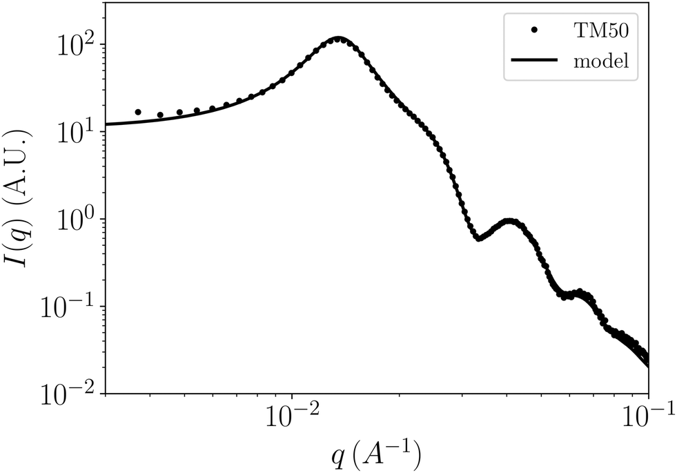Fig. 4 SAXS signal of the TM50 dispersion before compression (symbols) and corresponding model (line) for a reservoir salt concentration c_res = 5 mM. The optimized model parameters are: average radius a = 14.2 nm, polydispersity 1.46 nm, volume fraction ϕ = 0.082, pH = 9.02 (corresponding to a bare surface charge density σ = 0.42 e nm⁻²).

This spectrum has been fitted using eqn (1) with the following models for P(q) and S_m(q). Polydispersity has been accounted for using a Gaussian distribution for the radii in the form factor, which involves an average radius a and a polydispersity index. Computing a measurable structure factor is more involved. First, an effective interaction potential needs to be determined. Here we use a hard-sphere-Yukawa model u_eff depending on an effective colloidal charge Z_eff and on an effective screening length κ_eff⁻¹. These quantities were determined using a Poisson–Boltzmann (PB) cell model^33,34 for a monodisperse suspension of colloids with a radius equal to the average radius a. A simple one pK Stern model of colloidal surface chemistry was implemented in this cell model, so the bare surface charge density and the electrostatic potential around a colloid were computed self-consistently as a function of salt chemical potential and pH considering the surface reaction

Si–OH ⇌ Si–O⁻ + H⁺,

with an equilibrium constant corresponding to pK = 7.5, a Stern layer capacitance C_s = 2.9 F m⁻² and a total protonated and deprotonated site density Γ = 8 nm⁻². These parameters were considered fixed, and given by Trefalt and coworkers.³⁵ The solution of the PB cell model was then post-processed using the Extrapolated Point Charge (EPC) renormalization method³⁶ to obtain Z_eff and κ_eff⁻¹. To summarize, at the end of this step we have an effective potential accounting for both charge regulation and ion condensation, and their dependence on electrical double layer curvature and finite density effects, through the independent control parameters a, ϕ, and pH.

The measurable structure factor S_m(q) was then estimated as the structure factor S(q) of a monodisperse suspension of colloids with a radius equal to the average radius a at the same volume fraction. This function was obtained by solving the Ornstein–Zernike equation with the effective potential u_eff and the hypernetted-chain (HNC) closure. Identical results are obtained using the rescaled mean-spherical approximation (RMSA). We also tested a decoupling approximation^37,38 to include polydispersity effects in the structure factor calculation but it did not improve the results significantly. The monodisperse model S(q) was therefore used throughout this work for simplicity (see the ESI of ref. 27 more details concerning this approach).

Optimization of the free parameters of this model with respect to the SAXS data obtained before compression allowed to determine the average particle radius a = 14.2 nm, the size polydispersity 1.46 nm, the initial volume fraction of the suspension ϕ = 0.0822, and a pH of 9.02, which matches well the pH at which the suspension was prepared (pH = 9). These parameters yield an initial surface charge density of σ = 0.421 e nm⁻². The result of the fitting procedure matches the experimental data very closely (see Fig. 4). For comparison, Goehring and coworkers reported an average radius between 13.3 and 14.1 nm using different techniques and an identical polydispersity of 10%.^15,39

With the form factor measured in the “dilute” initial state, the structure factors of the suspension at higher volume fractions, after equilibration at 100, 150, and 200 mbar, could be extracted from the scattered intensities. They are reported in Fig. 5, together with one measurement by Chang and coworkers²³ which was conducted in conditions very close to those of our experiment at 100 mbar. Note that the experiment of Chang et al. was conducted on a synchrotron beamline, after weeks of classical osmotic compression. In both the present experiment at 100 mbar and Chang and coworker's experiment, we observe an essentially liquid-like structure with additional bumps located at the positions of the peaks of a body centered cubic (BCC) crystal. Such a structure has also been discussed by Bareigts and coworkers³² on the TM50 colloids used here. A notable difference between the structure factors reported by previous authors^23,32 and the one measured in the present microfluidic chip is the width of these additional BCC peaks. The peaks in the preliminary experiment at c_res = 1 mM reported in ESI† were thinner than those from the experiment reported here although the same X-ray beam and the same colloids were used. This rules out the influences of beam collimation and of polydispersity. The width of secondary peaks may also be influenced by the size of the crystallites. Here the half-width-half-maxima value δ ≃ 1 × 10⁻³ would suggest a crystallite size about π/δ ≃ 300 nm, which is outside the q range accessible by SAXS. The thinner peaks visible on Chang's curve would correspond to crystallites in the micrometer range. It could be possible that the time scale of our experiment did not allow to reach the same crystallite size as the one reported in ref. 23.

Fig. 5 Structure factors measured (crosses) and computed with liquid theory modeling (lines) ignoring the eventual existence of crystallites. The black dotted lines indicate the first theoretical BCC peak positions. The reservoir salt concentration was c_res = 5 mM, so κ_resa = 3.34. The dashed blue curve was taken from Fig. 10 in Chang et al.²³ for comparison, where ϕ = 0.23 and κ_resa = 3.33 (a = 10 nm, polydispersity 1.3 nm, c_res = 10 mM).

At a higher osmotic pressure of 150 mbar (and ϕ = 0.288), these peaks are barely discernible, and at 200 mbar (ϕ = 0.336) they seem to have completely disappeared. This crystal-to-glass transition upon concentration increase is consistent with previous results obtained on out-of-chip synchrotron runs and simulations, where the transition was found around ϕ = 0.25 at c_res = 5 mM.³² Predictions from the liquid theory are also reported in Fig. 5. They were obtained by fitting the volume fraction so the main peak position q_max is located at the correct q value, and by fitting the pH so the osmotic pressure in the model corresponds to the one imposed in the chip. The liquid theory model overestimates the main and secondary peak amplitudes because it cannot account for the presence of slightly denser and more ordered crystallites but it is consistent with the peak positions of the amorphous matrix.

Colloid volume fraction

In classical osmotic compression, measuring the volume fraction is straightforward: weigh a sample, dry it completely in an oven, and weigh it again. It is more delicate inside a microfluidic chip. If the colloids are dyed with fluorescent labels, optical microscopy can be used to infer the volume fraction after adequate calibration with known samples.²⁴ One drawback is that the tagging procedure usually involves playing with the surface chemistry of the colloids, which may alter in particular their electric charge and change the suspension properties. Another complication of this method when performing micro-structure measurements by SAXS is the need to implement a microscope on the X-ray setup.

The volume fractions reported above were determined by fitting the liquid theory model on the measured scattered intensities. Using this approach systematically on the different SAXS spectra obtained as a function of time yields the volume fraction evolution reported as a black curve in Fig. 6. The sometimes rough nature of this curve comes from the automatic fitting algorithm used on the ∼200 structure factors analyzed. As the present suspension sometimes contains BCC crystallites, we also used the relation

relating the volume fraction to the primary peak position of the structure factor in a perfect BCC crystal. The smooth evolution of this estimation reported in Fig. 6 as a blue line reflects the smooth evolution of q_max in this experiment. As in the present experiments we often observed a mixture of amorphous and crystalline phases, the average volume fraction lies somewhere between the BCC and liquid theory estimates, which are anyway quite close in the present strongly repulsive system.

Fig. 6 Volume fraction ϕ as a function of time during compression in the microfluidic chip. The different line colors correspond to different approaches to estimate the volume fraction, as described in the text. The black circles correspond to the 2D SAXS patterns reported in Fig. 3. Their ϕ value is the average of the “liquid” and “BCC” values.

Note that measuring ϕ by fitting the liquid theory to the SAXS spectra was achievable, though time consuming, because we utilized a well-known system of spherical, nearly monodisperse colloids for this proof of concept. However, the true value of exploring phase diagrams of colloidal suspensions using a microfluidic chip lies in studying systems that are not well understood, where a theoretical model is likely unavailable. Therefore, we will now discuss another approach to measure the colloid volume fraction.

A simple method to determine the volume fraction with the X-ray data is to compute the X-ray absorption based on the measured incident intensity I₀ and the transmitted intensity I(t) for each image. The absorbance follows Beer–Lambert's law

A(t) = ln(I₀/I(t)) = c + μ_wh(1 − ϕ(t)) + μ_shϕ(t), (2)

where c is the total absorbance of the walls of the chip, μ_w and μ_s are the linear attenuation coefficients of water and colloids, respectively, and h is the channel thickness. The reliable fit of the SAXS spectrum at initial time (Fig. 4) provides a reference value of ϕ allowing to fix c. Then the volume fraction estimated from sample absorbance at any time t isThe corresponding values reported in Fig. 6 as a grey line are consistent with the other estimation methods. The noise on these values is directly related to oscillations of the transmitted flux, which may be due to motions of the small crystallites inside the beam. Although this method yields results slightly more noisy than the other ones, it involves no a priori knowledge of the suspension and can therefore be used on any colloidal system.

Except when the volume fraction estimation based on absorbance fluctuates strongly for times larger than 50 hours, the difference between the three volume fraction estimations obtained with the different models was generally less than ±0.02 so the measurements were quite robust and consistent here.

Compression kinetics

Osmotic compression kinetics depend on the physico-chemical properties of the dispersion and on the device used. They are best discussed based on a Péclet number Pe = L[script L]_pΠ_i/D_i, where L is the length scale of the compression device, [script L]_p is the permeability of the membrane, Π_i is the initial osmotic pressure jump across the membrane, and D_i is the initial diffusion coefficient of the colloids.²⁴ This Péclet number compares the time scale for colloidal diffusion inside the drop L²/D_i and the time scale for meniscus displacement L/([script L]_pΠ_i). Here, L = 3.6 mm, the permeability of the membrane is supposed to be close to the one measured in our previous work²⁴ [script L]_p ≃ 2 × 10⁻¹² mPa⁻¹ s⁻¹, Π_i ≃ 0.1 bar, and the diffusion coefficient was estimated with the renormalized density fluctuation expansion of Beenakker and Mazur,^40–47 D_i ≃ 1.76 × 10⁻¹⁰ m² s⁻¹. These elements yield Pe ≃ 0.4, so both time scales are similar and we can estimate that the time to reach equilibrium in the device should be between L²/D_i ≃ 20 hours and L/([script L]_pΠ_i) ≃ 50 hours. The kinetics reported in Fig. 6 exhibit a first very fast volume fraction increase due to the fact that we imposed a very high pressure of 1 bar to speed up the concentration process (t < 7 h). After that, the relaxation events at 0.1, 0.15, and 0.2 bar are completely consistent with the time scale estimations above.

Note that this time scale to reach equilibrium is much larger than the 5 to 30 minutes achieved in our previous work using microfluidic osmotic compression without the constraints of in situ SAXS analysis.²⁴ Indeed, changes in the chip geometry were required to perform the SAXS experiments on a laboratory beamline: the initial colloidal drop length has been increased from 0.6 mm to 3.6 mm to allow the 0.25 mm beam size to fit into the drop even after a ten-fold compression, and the channel depth has been increased from 50 to 300 microns to increase the scattered to background intensity ratio. Therefore the volume of fluid to be exchanged through the membrane during a compression in the present chip was about 36 times larger than what could be realized without these constraints, while the membrane surface area involved in the exchange remained the same. Since at these small scales the water transfer kinetics are limited by the membrane permeability,²⁴ a 36-fold water volume increase induces a 36-fold transfer time increase, which is consistent with what was observed. Note that the present increase in drop size and channel depth were necessary to use a laboratory beamline, but a synchrotron X-ray source is much brighter and with a more focused beam so the present chip modifications would not be necessary in this context, and compression could be achieved in a few minutes with in situ micro-structure measurements. Finally, note that even if a compression step requires about 20 hours here, the device still allows for a continuous acquisition for different compression steps with a unique sample, without pipetting events that might disturb the micro-structure of the dispersion. It is therefore still a very valuable tool for the high-throughput screening of new colloidal formulations.

Equation of state

The equation of state (EOS) of colloidal suspensions, that is the evolution of the osmotic pressure as a function of volume fraction for fixed temperature and chemical potentials of the different ion species, is a useful macroscopic observable allowing to understand the mechanisms at play on the microscopic scale in different physico-chemical conditions. In this version of the microfluidic chip, osmotic pressure is imposed by the pressurization system and the volume fraction can be measured as described above, in particular with the X-ray absorbance method. EOS measurements are therefore quite straightforward, as they do not rely on the interpretation of the scattering data. Notably, they do not require any modeling or prior knowledge of the suspension. However, we will compare these experimental results with the predictions of liquid theory, as this comparison highlights a significant issue related to pH control in these microfluidic experiments.

To compute the osmotic pressure, we first compute the suspension meso-structure (in the form of S(q) or g(r)) by solving the OZ equation with an effective potential determined as introduced above. The osmotic pressure is then³⁶

where the first two terms constitute the standard virial pressure and the last one is introduced by the use of EPC renormalization. The very good accuracy and predictive capacity of this model can be verified by comparing its EOS predictions to the data from compression by standard dialysis at 0.5 and 5 mM reservoir salt concentrations obtained by Goehring and coworkers using a classical dialysis technique and a synchrotron for SAXS measurements, as shown in ESI.†^15,32 The input parameters of the model are the volume fraction, the colloid radius determined experimentally from scattering data, and the salt reservoir concentration and pH which are in principle controlled experimental parameters.

The Π(ϕ) data sets measured at equilibrium in microfluidic chips are reported in Fig. 7 for two different salt reservoir concentrations, together with theoretical results. The initial states (volume fractions) of the dispersion drops at c_res = 1 and 5 mM introduced inside the microfluidic chips are indicated with blue and red crosses, respectively. They were purposely set quite far from the equilibrium values, and arrows show the path followed by the dispersion during compression inside the microfluidic chip. Open circles are the stationary states obtained for each pressure step. For the experiment reported in red, the salt solution in the reservoir was prepared at pH = 10 and c_res = 5 mM. Agreement is very good with theory at pH = 10 for the first pressure step at 100 mbar reached after 17 hours, as expected. The volume fractions reached during the next two pressure steps at 150 and 200 mbar and obtained after 40 and 60 hours of compression appear to lie on equations of state corresponding to pH = 8.5 and 7.75, respectively. These results suggest a slow acidification of the salt reservoir with time. This is confirmed in the experiment at c_res = 1 mM reported in blue, where the first two data points are in good agreement with the theoretical values taken at pH = 10. The first data point was obtained after 27 hours of operation, and the second point was obtained after approximately 10 hours of aging the salt solution, following a refill of the salt reservoir in between. The final data point in this experiment appears to align with the equation of state for pH = 8.3, after 80 hours of aging the salt solution.

Fig. 7 Equation of state of TM50 colloids measured in the present microfluidic chip (open symbols), and calculated theoretically (lines, see main text for the details). For calculations, a = 14.2 nm. The two crosses show the initial volume fraction of the suspension and do not correspond to equilibrium data. The black arrows show the path followed by the dispersion in the microfluidic chip.

Water acidification due to CO₂ absorption is well known when it is left exposed to the atmosphere but we did not expect this to occur in the closed Fluigent pressurization cells. The pH was therefore not monitored during the compression experiments, but pH measurements have been conducted a posteriori in pressurized and non-pressurized cells over the course of 120 hours. Results reported in ESI† show that the pressurization cells indeed allow for acidification of the water they contain, either because they cannot be considered as completely airtight, or because they generate some gas motion accelerating CO₂ gas/liquid transfer inside the tubes. The rate at which the pH shifts may depend on the imposed pressure, on the seal model and condition, and on the tightening of the cap, so we did not pursue this issue further. Several solutions are possible to have a good control of the pH for experiments running over a few days: add an inert oil cap above the water in the pressurized tubes, use a CO₂ trap before the pressurization system inlet, use nitrogen as pressurizing gas, or use syringe pumps.

Comparison to other EOS measurement methods

To conclude this discussion, a comparison of the strengths and weaknesses of the present microfluidic method with other well established methods to determine osmotic pressures in colloidal dispersions is in order. The closest alternative method is membrane osmometry (see e.g. ref. 48 and references therein). The present microfluidic chip being in essence a miniaturized membrane osmometer, their weaknesses are in part similar. In particular, the membrane must not be deteriorated by the solvent. It should also have very small pores or even be dense if the colloids are small (polymers, some quantum dots or small proteins…). Although we could produce such membranes by removing partially or even totally the pore-forming component, their permeability to water becomes very low and equilibration times increase. In its present form, the microfluidic device is thus not well suited to the study of polymers or metallic colloids dissolved in organic solvents for example. The other major method to determine colloidal EOSs is analytical centrifugation,^6,12,49,50 in which a dispersion is centrifuged until an equilibrium concentration gradient emerges from a balance between “hydrostatic” and osmotic pressures. Interestingly, this method can be used with any solvent and colloids and yields a full equation of state in a single experiment, which can last a few tenth minutes. This method also handles well less stable suspensions that may aggregate at large volume fractions: dense phases will simply be present below more stable phases. However it requires sample volumes of a few mL, does not allow the exchange of small species with a controlled reservoir, and it could hardly be used for simultaneous characterization by SAXS. Compared to membrane osmometry and analytical centrifugation, the most significant advantages of the present microfluidic device are the very small sample volumes required, which allow to speed up the equilibration process and the study of expensive materials, and the flowing salt reservoir allowing a precise control of the chemical potentials of small dissolved species. Special care might be needed if less stable suspensions are to be studied. Indeed, the chip and membrane will be fouled if colloids aggregate irreversibly, with no efficient means for cleaning.

Conclusion and perspectives

We have developed an innovative microfluidic design for the osmotic compression of suspensions at the nanoliter scale, enabling the acquisition of in situ and operando structural features throughout the compression process. This design builds upon a previous set-up that operated without simultaneous X-ray scattering measurements.²⁴

In this updated chip design, several modifications have been implemented to facilitate small-angle X-ray scattering (SAXS) measurements on a laboratory beamline. Specifically, the thickness of the OSTEMER walls has been reduced to 50 μm to minimize undesired absorption and scattering. The thickness of the sample-containing channel has been increased to 300 μm to enhance the scattering from the sample, and its width has also been expanded to 300 μm to accommodate the X-ray beam size. Additionally, the channel length has been extended to 3.6 mm, allowing for ten-fold compressions. Because photo-polymerization of a membrane could not be reliably achieved in 300 μm thick channels, a 3D channel design was introduced with the membrane synthesized in a smaller 50 μm high section of the channel.

To evaluate the new design, we performed osmotic compression experiments on Ludox TM50 silica suspensions, which had previously been characterized using standard macroscopic osmotic compression techniques and analyzed with synchrotron radiation. Structural analysis revealed the presence of amorphous phases or mixtures of amorphous and FCC or BCC crystalline phases, aligning with prior observations. These results validate the capability of the setup to establish phase diagrams using a single nanoliter-scale sample, provided the structural transitions are reversible.

The equation of state (EOS) of colloidal suspensions is the other major critical type of data that can be obtained with this setup. We demonstrated that the volume fraction can be tracked over time during compression, either by monitoring X-ray absorbance or by modeling the scattered signals. The former method is universally applicable, even to unknown samples, while the latter requires some prior knowledge of the suspension, such as particle anisotropy or surface reactions. As the osmotic pressure and salt chemical potential are precisely controlled, EOSs can be determined unambiguously from the volume fraction measurements. The shapes of EOSs themselves can already inform qualitatively on phase transitions, offering insights in many practical applications. EOSs can also be compared with existing or new thermodynamic models on more academic topics, such as the determination of effective interaction potentials.

The primary drawback of the present microfluidic chips is their slower compression kinetics, approximately 20 hours per pressure step, compared to the 5–20 minutes per step achieved with chips designed for use under a microscope without simultaneous structure measurements. This difference is due to the increased channel depth and length required for use with a laboratory beamline. When several pressure steps are imposed sequentially, as in this study, continuous measurements over several days require careful pH control in the reservoirs, particularly if pH influences the colloidal suspension being investigated.

This drawback is offset by several significant advantages: (i) the current compression times are still considerably shorter than those required by the traditional osmotic compression technique (1–2 weeks); (ii) most of the benefits of microfluidics, such as small sample volumes and precise control, are retained while offering easier access to laboratory beamlines compared to synchrotron facilities; (iii) the same chip design, but with smaller channels, could be adapted for use with synchrotron sources, enabling compressions on time scales of just a few minutes; (iv) compared to the initial design presented in ref. 24, colloidal particles in the suspension no longer need to be labeled to measure their volume fraction. This is particularly valuable when the surface chemistry of the colloids governs inter-particle interactions, for example in mineral oxide suspensions or dispersions of colloids of biological origin, including proteins and lipid nano-particles.

These microfluidic chips will be valuable for understanding the behavior of colloidal suspensions, particularly when the chemical potential of the small dissolved species, such as ions, needs to be controlled precisely through the membrane. They will find applications in areas such as crystallization, nucleation, soil mechanics, control of living matter growth and interaction conditions, as well as the measurement of coarse-grained colloidal interaction potentials.

Data availability

The data supporting this article have been included as part of the ESI† in the archive named Radajewski2024_data.zip.

Author contributions

D. R. is the primary contributor who designed and built the microfluidic chips, and performed the scattering experiments. P. R. developed the SAXS equipment and performed the SAXS acquisition. M. M. and Y. H. contributed to SAXS data acquisition. Y. H. performed most of the modelling. M. M. and Y. H. supervised this work. All parties contributed to the review and editing of the manuscript.

Conflicts of interest

There are no conflicts to declare.

Acknowledgements

We thank J.-B. Salmon, I. Rodriguez-Ruiz, and S. Teychené for discussions concerning the microfluidic chip development. We acknowledge the ANR program Grant No. ANR-18-CE06-0021 for financial support.

Notes and references

1. R. Roy, Science, 1987, 238, 1664–1669.
2. T. F. Tadros, Adv. Colloid Interface Sci., 1993, 46, 1–47.
3. A. Mihranyan, N. Ferraz and M. Strømme, Prog. Mater. Sci., 2012, 57, 875–910.
4. R. Moreno, J. Eur. Ceram. Soc., 2020, 40, 559–587.
5. Z. Cai, Z. Li, S. Ravaine, M. He, Y. Song, Y. Yin, H. Zheng, J. Teng and A. Zhang, Chem. Soc. Rev., 2021, 50, 5898–5951.
6. E. L. Hansen, H. Hemmen, D. d. M. Fonseca, C. Coutant, K. Knudsen, T. Plivelic, D. Bonn and J. O. Fossum, Sci. Rep., 2012, 2, 618.
7. C. Bonnet-Gonnet, L. Belloni and B. Cabane, Langmuir, 1994, 10, 4012–4021.
8. C. Martin, F. Pignon, A. Magnin, M. Meireles, V. Lelièvre, P. Lindner and B. Cabane, Langmuir, 2006, 22, 4065–4075.
9. A. Mourchid, A. Delville, J. Lambard, E. Lecolier and P. Levitz, Langmuir, 1995, 11, 1942–1950.
10. A. Robbes, F. Cousin and G. Mériguet, Braz. J. Phys., 2009, 39, 156–162.
11. J. Li, B. Cabane, M. Sztucki, J. Gummel and L. Goehring, Langmuir, 2012, 28, 200–208.
12. R. Piazza, T. Bellini and V. Degiorgio, Phys. Rev. Lett., 1993, 71, 4267.
13. P. Pusey, H. Fijnaut and A. Vrij, J. Chem. Phys., 1982, 77, 4270–4281.
14. Y. Hallez, J. Diatta and M. Meireles, Langmuir, 2014, 30, 6721–6729.
15. L. Goehring, J. Li and P.-C. Kiatkirakajorn, Philos. Trans. R. Soc., A, 2017, 375, 20160161.
16. P. Bacchin, D. Brutin, A. Davaille, E. Di Giuseppe, X. D. Chen, I. Gergianakis, F. Giorgiutti-Dauphiné, L. Goehring, Y. Hallez and R. Heyd, et al., Eur. Phys. J. E: Soft Matter Biol. Phys., 2018, 41, 1–34.
17. W. Russel, J. Rheol., 1980, 24, 287–317.
18. Y. Hallez, I. Gergianakis, M. Meireles and P. Bacchin, J. Rheol., 2016, 60, 1317–1329.
19. B. Cabane, J. Li, F. Artzner, R. Botet, C. Labbez, G. Bareigts, M. Sztucki and L. Goehring, Phys. Rev. Lett., 2016, 116, 208001.
20. L. Feigin and D. I. Svergun, et al., Structure analysis by small-angle X-ray and neutron scattering, Springer, 1987, vol. 1.
21. O. Glatter, O. Kratky and H. Kratky, Small angle X-ray scattering, Academic press, 1982.
22. A. Guinier, G. Fournet and K. L. Yudowitch, Small-angle scattering of X-rays, Wiley, New York, 1955.
23. J. Chang, P. Lesieur, M. Delsanti, L. Belloni, C. Bonnet-Gonnet and B. Cabane, J. Phys. Chem., 1995, 99, 15993–16001.
24. C. Keita, Y. Hallez and J.-B. Salmon, Phys. Rev. E, 2021, 104, L062601.
25. D. Kleshchanok, P. Holmqvist, J.-M. Meijer and H. N. W. Lekkerkerker, J. Am. Chem. Soc., 2012, 134, 5985–5990.
26. M. A. Levenstein, K. Robertson, T. D. Turner, L. Hunter, C. O'Brien, C. O'Shaughnessy, A. N. Kulak, P. Le Magueres, J. Wojciechowski, O. O. Mykhaylyk, N. Kapur and F. C. Meldrum, IUCrJ, 2022, 9, 538–543.
27. D. Radajewski, P. Roblin, P. Bacchin, M. Meireles and Y. Hallez, Lab Chip, 2023, 23, 3280–3288.
28. C. E. Hoyle and C. N. Bowman, Angew. Chem., Int. Ed., 2010, 49, 1540–1573.
29. D. Radajewski, L. Hunter, X. He, O. Nahi, J. M. Galloway and F. C. Meldrum, Lab Chip, 2021, 21, 4498–4506.
30. T. Lange, S. Charton, T. Bizien, F. Testard and F. Malloggi, Lab Chip, 2020, 20, 2990–3000.
31. J. Decock, M. Schlenk and J.-B. Salmon, Lab Chip, 2018, 18, 1075–1083.
32. G. Bareigts, P.-C. Kiatkirakajorn, J. Li, R. Botet, M. Sztucki, B. Cabane, L. Goehring and C. Labbez, Phys. Rev. Lett., 2020, 124, 058003.
33. S. Alexander, P. Chaikin, P. Grant, G. Morales, P. Pincus and D. Hone, J. Chem. Phys., 1984, 80, 5776–5781.
34. E. Trizac, L. Bocquet, M. Aubouy and H.-H. von Grünberg, Langmuir, 2003, 19, 4027–4033.
35. G. Trefalt, S. H. Behrens and M. Borkovec, Langmuir, 2016, 32, 380–400.
36. N. Boon, G. I. Guerrero-García, R. Van Roij and M. Olvera de la Cruz, Proc. Natl. Acad. Sci. U. S. A., 2015, 112, 9242–9246.
37. M. Kotlarchyk and S.-H. Chen, J. Chem. Phys., 1983, 79, 2461–2469.
38. G. Nägele, Phys. Rep., 1996, 272, 215–372.
39. P.-c. Kiatkirakajorn, PhD thesis, Georg-August-Universität Göttingen, 2018.
40. C. Beenakker and P. Mazur, Phys. Lett. A, 1983, 98, 22–24.
41. C. Beenakker and P. Mazur, Phys. A, 1984, 126, 349–370.
42. C. Beenakker, Phys. A, 1984, 128, 48–81.
43. U. Genz and R. Klein, Phys. A, 1991, 171, 26–42.
44. A. J. Banchio and G. Nägele, J. Chem. Phys., 2008, 128(10), 104903.
45. M. Heinen, P. Holmqvist, A. J. Banchio and G. Nägele, J. Chem. Phys., 2011, 134, 044532.
46. F. Westermeier, B. Fischer, W. Roseker, G. Grübel, G. Nägele and M. Heinen, J. Chem. Phys., 2012, 137(11), 114504.
47. J. Riest and G. Nägele, Soft Matter, 2015, 11, 9273–9280.
48. C. S. Hale, D. W. McBride, R. Batarseh, J. Hughey, K. Vang and V. Rodgers, Rev. Sci. Instrum., 2019, 90, 034102.
49. D. Carrière, M. Page, M. Dubois, T. Zemb, H. Cölfen, A. Meister, L. Belloni, M. Schönhoff and H. Möhwald, Colloids Surf., A, 2007, 303, 137–143.
50. M. G. Page, T. Zemb, M. Dubois and H. Cölfen, ChemPhysChem, 2008, 9, 882–890.

---

Footnote

† Electronic supplementary information (ESI) available. See DOI: https://doi.org/10.1039/d4lc01087f

---