 Open Access Article
Creative Commons Attribution 3.0 Unported Licence
Precisely controlled colloids: a playground for path-wise non-equilibrium physics
Cai
Dieball
 a,
Yasamin
Mohebi Satalsari
b,
Angel B.
Zuccolotto-Bernez
b,
Stefan U.
Egelhaaf
 b,
Manuel A.
Escobedo-Sánchez
 *b and
Aljaž
Godec
 *a
*a
aMathematical bioPhysics Group, Max Planck Institute for Multidisciplinary Sciences, 37077 Göttingen, Germany. E-mail: agodec@mpinat.mpg.de
bCondensed Matter Physics Laboratory, Heinrich Heine University Düsseldorf, 40225, Düsseldorf, Germany. E-mail: escobedo@hhu.de
First published on 14th February 2025
Abstract
We investigate path-wise observables in experiments on driven colloids in a periodic light field to dissect selected intricate transport features, kinetics, and transition-path time statistics out of thermodynamic equilibrium. These observables directly reflect the properties of individual paths in contrast to the properties of an ensemble of particles, such as radial distribution functions or mean-squared displacements. In particular, we present two distinct albeit equivalent formulations of the underlying stochastic equation of motion, highlight their respective practical relevance, and show how to interchange between them. We discuss conceptually different notions of local velocities and interrogate one- and two-sided first-passage and transition-path time statistics in and out of equilibrium. Our results reiterate how path-wise observables may be employed to systematically assess the quality of experimental data and demonstrate that, given sufficient control and sampling, one may quantitatively verify subtle theoretical predictions.
1 Introduction
Colloidal particles, due to their high susceptibility to external fields, can be precisely manipulated using light,1–12 electrical and magnetic fields,1,13–15 or microfluidic devices.16 This makes them an ideal platform to validate fundamental physical theories of soft matter with a high degree of accuracy. Over the years, substantial effort has been made in colloidal soft matter to explore various aspects of both stochastic dynamics17–20 and stochastic thermodynamics.21,22 In fact, colloidal systems have always served as a paradigm for stochastic thermodynamics,21,22 which generalizes the notion of thermodynamic observables to individual stochastic paths. Many fundamental kinetic and thermodynamic properties have been discovered and verified using colloids, including the statistics of work performed on23,24 and heat dissipated by24 a driven colloid, detailed25 and transient26 fluctuation theorems, realizations of heat engines,6,11,12 as well as first-passage8,27,28 and transition-path time statistics,29–33 to name a few. Notably, these are properties of individual stochastic paths, so-called functionals, which inherently provide much deeper insight into the underlying dynamics than their ensemble-average counterparts.34–40Despite decades of intensive research leading to numerous significant discoveries, the potential of driven and controlled colloids to reveal fundamental physical laws remains far from exhausted. On the one hand, this may be because advances in abstract theory (e.g., functional fluctuation relations,39,41,42 speed limits,43–46 thermodynamic uncertainty relations45,47–56) do not so easily proliferate to experiments or require excellent statistics. On the other hand, reciprocal-space-based techniques (e.g., dynamic light scattering, neutron or X-ray scattering, differential dynamic microscopy and variants)57–60 are only beginning to be considered in the theory of stochastic thermodynamics.46
To go beyond the state-of-the-art in particle-tracking analysis we focus on path-wise observables that directly reflect properties of entire individual paths rather than properties of the probability density of an ensemble of particles, such as radial distribution functions or mean-squared displacements. Path-wise refers to those functionals of particular realizations of trajectories that map entire trajectories (Xτ)0≤τ≤t or large parts of them to some f[(Xτ)0≤τ≤t], as opposed to observables depending only on the value at some fixed set of times, e.g., f(Xτ1,Xτ2). A particular class of insightful path-wise observables is first-passage time,61,62 which is the stochastic time it takes for a trajectory to reach a prescribed target (position) for the first time, e.g., f[(Xτ)0≤τ≤t] = arg min0≤τ≤∞(Xτ = a) for a target at a. For example, first-passage time statistics have been shown to provide a deeper understanding of the origin of sub-diffusion than mean-squared displacements.63 Moreover, they can distinguish processes with equal transition probability densities,64 unravel the number of intermediate states,28 and reveal fractal dynamics of colloids.8 Related, albeit quite different, path-wise observables are transition-path times defined as the stochastic duration of successful transitions, whereby “successful” reflects that the particle does not return to its original position before arriving at a predefined target point.65–68 Under typical conditions, transition-path times obey a surprising symmetry,65 and violations of this symmetry may be used to gain intriguing insights.31
The “inherent” sensitivity of the selected observables is such that they can be systematically used to assess and critically verify the quality of experimental data. In this study, we conduct precise experiments on colloids driven through a periodic light field to investigate fundamental and complex aspects of transport, along with first-passage and transition-path times in out-of-equilibrium conditions. Our results reiterate how given sufficient control and sampling even the most subtle theoretical predictions may be verified quantitatively, which will hopefully reinforce the motivation in the field of experimental soft matter to test and further increase the quality of experimental data.
1.1 Structure of the paper
In the first part, we present two different ways to write the underlying stochastic equation of motion on a trajectory-based level and show how to interchange between the two in theory and practice. We highlight the necessity of knowing both representations by connecting them to essential dynamic and thermodynamic properties. Based on these representations, we discuss conceptually different notions of local velocities, whose interrelations are a priori not obvious. Next, we investigate first-passage time statistics for barrier-crossing events and show how these are linked to the local mean velocity (using ref. 69). Finally, we verify (and slightly extend to periodic systems) the transition-path time symmetry predicted in ref. 65,68. All of the aforementioned aspects are confirmed and supported by experimental data on both equilibrium (passive) and driven experiments. We conclude with a perspective on further research directions and open questions.2 Materials and methods
In this study, the applied potential is periodic in the x-direction and originates from the optical force resulting from the interaction of particles with a periodic light field with period L = 4.135 μm.2.1 Sample preparation
We prepared a dilute colloidal dispersion containing polystyrene Sulfate latex particles of 1.5 μm radius with a polydispersity of 4% (Thermo Fisher Scientific, batch number 1660463). The particles were suspended in ultra-pure water with a resistivity of 18.2 MΩ cm (Purelabs Flex, Elga). The dispersion was confined to quasi-two-dimensional (2D) sample cells, which were assembled as follows: 2.3 μL of the dilute colloidal dispersion was placed on top of a 22 × 50 mm cover slip, then a 22 × 22 mm cover slip was carefully placed on top, and the slides were glued together using UV-curing glue (NOA61, Norland Products Inc.). We mounted the assembled cell on a microscope slide. To avoid the two glasses to get too close to each other (by capillary forces) and pinning the particles, we have used the polydispersity of the sample, i.e., the larger sizes in the dispersion (particles of around 2 μm in radius), as spacers. All sample cells were left to reach equilibrium in a laboratory environment at 20 °C for two days. The area fraction was φa ≃ 1%.2.2 Experimental setup
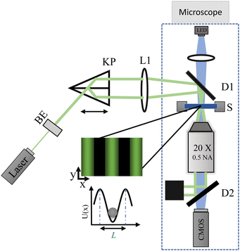
In this study, the periodic light field is created by the interference of two laser beams.70 A laser beam (Cobolt 05-01 Samba 1.5 W) of 532 nm wavelength, is expanded and then split into two parallel beams using a Köster prism. Using a lens and a dichroic mirror the beams are guided to interfere on the microscope sample plane, creating a fringe pattern. The period (L, dark-bright fringe) can be changed by moving the Kösters prism position. The laser beams are removed from the image path (with a dichroic mirror) and a CMOS camera (Mako U-130B) is used as sensor to record images. The sample cell sits on a piezo nanopositioner stage (Mad City Labs, Nano-BioS300), which is used to move the sample. A schematic representation of the experimental setup is shown in Fig. 1. For details on the extraction of the period L and amplitude of the potential, see Appedix A.2.3 Optical microscopy and particle tracking
All experiments were performed with the colloidal particles under the effect of the periodic light field.![[thin space (1/6-em)]](https://www.rsc.org/images/entities/char_2009.gif) 000 images per measurement. This corresponds to a total measurement duration of 1 hour. We conducted several experiments that reached a total collection of 1224 trajectories. We used modified MATLAB-based particle tracking routines based on those of D. Blair and E. Dufresne71 to accurately determine the position of the colloids. Additionally, by following the Michalet algorithm,72 we estimated the localization uncertainty to be ±2 nm. For a direct comparison to the driven state experiments, we treated the 1224 trajectories as 2448 trajectories with a duration of 30 minutes each.
000 images per measurement. This corresponds to a total measurement duration of 1 hour. We conducted several experiments that reached a total collection of 1224 trajectories. We used modified MATLAB-based particle tracking routines based on those of D. Blair and E. Dufresne71 to accurately determine the position of the colloids. Additionally, by following the Michalet algorithm,72 we estimated the localization uncertainty to be ±2 nm. For a direct comparison to the driven state experiments, we treated the 1224 trajectories as 2448 trajectories with a duration of 30 minutes each.
![[thin space (1/6-em)]](https://www.rsc.org/images/entities/char_2009.gif) 500 steps, with a 40 ms pause between each step. Optimizing these values allowed us to drag the sample cell at a controlled velocity of v0 = (0.053 ± 0.002) μm s−1. We recorded images at 25 frames per second, each measurement containing 45
500 steps, with a 40 ms pause between each step. Optimizing these values allowed us to drag the sample cell at a controlled velocity of v0 = (0.053 ± 0.002) μm s−1. We recorded images at 25 frames per second, each measurement containing 45![[thin space (1/6-em)]](https://www.rsc.org/images/entities/char_2009.gif) 000 images, for a total measurement time of 30 minutes. In total, we acquired 1168 trajectories.
000 images, for a total measurement time of 30 minutes. In total, we acquired 1168 trajectories.
3 Overdamped Langevin dynamics in a periodic drift field
3.1 Equilibrium dynamics
The dynamics of colloidal particles are generically overdamped on the observed scales.17 Thus, we consider the stochastic dynamics in one-dimensional space of a colloidal particle with position Xt connected to a thermal bath with temperature T, governed by the overdamped Langevin equation | (1) |
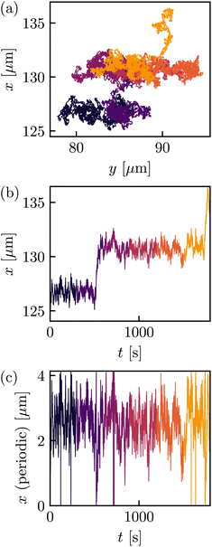
As mentioned in Section 2, in this study, the potential U(x) is periodic in the x-direction with a period L. An experimental trajectory is shown in Fig. 2. Note that the motion in the y-direction will only correspond to a free Brownian motion, as there is no force coming from U(x) in this direction. The latter is illustrated in Fig. 2(a) where the effect of U(x) constrains the movement in the x-direction, contrary to the y-direction where it is allowed to move freely.
In Fig. 2(b) and (c), we therefore focus onXt, where in (c) we show xt which is defined as Xt projected onto a single period [0,L), i.e., xt ≡ Xt![[thin space (1/6-em)]](https://www.rsc.org/images/entities/char_2009.gif) mod
mod![[thin space (1/6-em)]](https://www.rsc.org/images/entities/char_2009.gif) L. Accordingly, for U(x) = U(x + L) we may view eqn (1) as L-periodic dynamics for xt, i.e.,
L. Accordingly, for U(x) = U(x + L) we may view eqn (1) as L-periodic dynamics for xt, i.e.,  with the definition xt+dt ≡ (xt + dxt)
![[thin space (1/6-em)]](https://www.rsc.org/images/entities/char_2009.gif) mod
mod![[thin space (1/6-em)]](https://www.rsc.org/images/entities/char_2009.gif) L ensuring that xt remains confined to [0,L).
L ensuring that xt remains confined to [0,L).
If projected on [0,L), the system settles into a Boltzmann equilibrium density peq(x) ∝ exp(−U(x)/kBT).73
More generally, not all systems settle into equilibrium steady states. For sufficiently confined systems and drifts without an explicit time dependence, a steady state is approached for t → ∞. Similarly, for space-periodic dynamics treated as if they evolve in a single period, i.e., projected onto a single period, a steady state is approached for long times, assuming no explicit time dependence in the drift and diffusion. However, here, a stationary current emerges if the system is driven out of equilibrium by a non-conservative drift; see below.
3.2 Driven dynamics
While equilibrium dynamics are interesting and important, they are relatively well understood. However, they do not apply to irreversible (e.g., living) systems since these are inherently out of equilibrium, e.g., driven by non-conservative flows (i.e., shear) or ATP hydrolysis. Note that the theory presented here is not new but is simply presented in a comprehensive manner and in a potentially new logical order to stay close to the experiment. To address driven dynamics, we consider the simplest situation in which we add a constant bare velocity v0 in the x-direction to the Langevin eqn (1), yielding | (2) |
In the experiments, v0 is introduced by dragging the sample cell with a constant velocity −v0 along the periodic direction of U(x) using the piezo nanopositioner stage. For a sample trajectory in this driven setting, see Fig. 3. Note that, as before, the motion in the x- and y-directions decouples and that the motion in the y-directions remains equilibrium Brownian motion only, see Fig. 3(a).
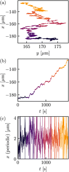 | ||
| Fig. 3 Example of a trajectory that is driven by ν0, see eqn (2), (a), and corresponding projection onto the x-axis (b) and (c) where time runs from dark to bright. (c) The period is always chosen as L = 4.135 μm. The dataset comprises 1168 such trajectories. | ||
What can we say about the driven dynamics? First, the dynamics projected onto a single period, see Fig. 3(c), still settles into a steady state—a non-equilibrium steady state (NESS)—with density ps(x), which, however, no longer has a Boltzmann form. Instead, the shape of ps(x) is skewed in the direction of sign (v0).
The first question that arises is, given eqn (2), what is ps(x) for a given bare velocity v0 ≠ 0? The second question refers to the movement (i.e., probability current) of the driven particle; see Fig. 3(b). This question is non-trivial, and compared to the bare velocity v0, the particle is expected to slow down by the barriers of U(x). Thus, one naturally wonders what theoretical velocity is implied by the equation of motion in eqn (2).
Both questions can be answered by rewriting eqn (2) into an alternative form
 | (3) |
In the following subsection, we will show how to derive it. First, we will discuss the properties and usefulness of this rewriting. Here, js is the steady-state probability current and νs(x) ≡ js/ps(x) is the “local mean velocity”.22 The latter has to fulfill ∂x[νs(x)ps(x)] = 0 to ensure that ps(x) is indeed the steady state density, which is seen by requiring that ∂tp(x,t) = 0 for p(x,t) = ps(x), where p(x,t) is the probability density goverend by the Fokker–Planck equation,73,74
| ∂tp(x,t) = −∂x{[−D∂xU(x)/kBT + v0 − D∂x]p(x,t)} |
= −∂x{[D∂xln![[thin space (1/6-em)]](https://www.rsc.org/images/entities/char_2009.gif) p(x,t) + ν(x,t) − D∂x]p(x,t)} p(x,t) + ν(x,t) − D∂x]p(x,t)} |
| = −∂x[ν(x,t)p(x,t)]. | (4) |
In one-dimensional space, this directly implies that there is a constant probability current js with νs(x) = js/ps(x). For equilibrium dynamics v0 = 0, js = 0, and thus both presentations eqn (2) and (3) agree, since for the equilibrium density peq(x) we have ∂xln![[thin space (1/6-em)]](https://www.rsc.org/images/entities/char_2009.gif) peq(x) = −∂xU(x)/kBT. Thus, both can be seen as a direct extension of eqn (1).
peq(x) = −∂xU(x)/kBT. Thus, both can be seen as a direct extension of eqn (1).
Eqn (3) is particularly insightful when considering microscopic reversibility (i.e., detailed balance) and its generalizations. Namely, if we let Gνs(x,t|x0) denote the two-point conditional probability density of xt (which is the Green's function of the Fokker–Planck eqn (4), i.e., ∂tGνs = −∂x[−D∂xln![[thin space (1/6-em)]](https://www.rsc.org/images/entities/char_2009.gif) ps(x) + νs(x)]Gνs with Gνs(x,0|x0) = δ(x − x0)), then detailed balance corresponds to
ps(x) + νs(x)]Gνs with Gνs(x,0|x0) = δ(x − x0)), then detailed balance corresponds to
| G0(x,t|x0)ps(x0) = G0(x0,t|x)ps(x). | (5) |
This indeed holds if and only if νs(x) = 0 (i.e., js = 0). In contrast, the generalization of eqn (5)–the so-called “dual reversal” symmetry-corresponds to40
| Gνs(x,t|x0)ps(x0) = G−νs(x0,t|x)ps(x). | (6) |
Note that the dual reversal symmetry eqn (6) and symmetries of dynamical functionals of xt (see ref. 40) are only applicable to the steady-state local mean velocity νs(x) in eqn (3) but not to the bare velocity v0 in eqn (2). On the other hand, the potential U(x) that enters thermodynamic potentials only appears in the first form (2). The main difference between the representations eqn (2) and (3) is that the additional term νs(x) = js/ps(x) (unlike v0) does not alter the steady-state density ps(x), irrespective of the value of the constant steady-state current js.
When discussing the velocity of the driven system, we must note that ẋt does not exist in a mathematical sense for overdamped motion as in eqn (2) and (3) [technically Prob(|ẋt| < C) = 0 for all C < ∞] and that there are, in fact, different notions of velocity. The bare velocity v0 and the drift velocity vdrift(x) (where 〈·|xτ = x〉 denotes the average conditioned on xτ = x for any τ ∈ [0,t]),
 | (7) |
![[small nu, Greek, macron]](https://www.rsc.org/images/entities/i_char_e0ce.gif) ,
, | (8) |
![[small nu, Greek, macron]](https://www.rsc.org/images/entities/i_char_e0ce.gif) as t → ∞. Moreover, note that for a periodic U(x) (with known period L), the mean velocity is equivalently characterized by the following expressions (recall that Xτ is the full dynamics and xτ ≡ Xτ
as t → ∞. Moreover, note that for a periodic U(x) (with known period L), the mean velocity is equivalently characterized by the following expressions (recall that Xτ is the full dynamics and xτ ≡ Xτ![[thin space (1/6-em)]](https://www.rsc.org/images/entities/char_2009.gif) mod
mod![[thin space (1/6-em)]](https://www.rsc.org/images/entities/char_2009.gif) L),
L), | (9) |
 to show 〈vdrift(xτ)〉s = 〈νs(xτ)〉s as well as
  (see, e.g., ref. 40 for details). The term τ(x → x + L) in eqn (9) denotes the first-passage time from x to x + L, i.e., the (stochastic) time that a trajectory (Xτ)0≤τ≤t starting at position x takes to reach position x + L for the first time, see also Fig. 7. The last equality in eqn (9) is shown in ref. 69 and will be revisited later in this work. Before we demonstrate and verify the different notions of velocities from the experimental data, we first need to find a way to swap between the representations, that is, from eqn (2) to eqn (3) and vice versa.
3.3 Swapping representations: From eqn (2) to eqn (3)
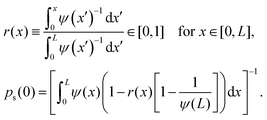
On a general note, we emphasize that determining eqn (3) analytically in a high-dimensional space is generally not feasible (i.e., it requires solving the stationary Fokker–Planck equation ∂tp(x,t) = 0; in practice, one would need to simulate long trajectories and estimate ps(x) as histograms). However, in the given one-dimensional scenario with constant bare velocity v0 there is a way to obtain ps(x) and, consequently, eqn (3) from eqn (2), see ref. 73, which we follow here.Define the auxiliary function ψ(x) (here 0 is the left side of the periodic interval, and x ∈ [0,L]) as
 | (10) |
The result for ps(x) is
| ps(x) = ps(0)ψ(x)(1 − r(x)[1 − ψ(L)−1]), | (11) |
 | (12) |
As a consistency check, we note that for v0 = 0 we should recover the Boltzmann distribution, and indeed we find ψ(x) = exp([U(0) − U(x)]/kBT) such that ψ(L) = e0 = 1 and ps(x)/ps(0) =ψ(x) provides it. Additionally, in Fig. 4(a), we also verify eqn (3) as its resulting ps (dashed line) overlaps with the ps measured from a histogram of the driven dynamics (red line) with experimental data.
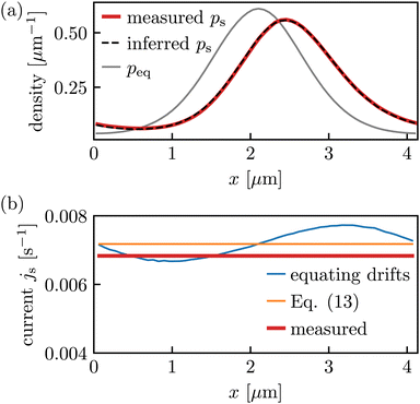 | ||
Fig. 4 (a) ps(x) in eqn (11) inferred from equilibrium (passive) experiments and using the value ν0= 0.053 μm s−1 of the experimentally fixed velocity, where we deduced U(x)/kBT up to a constant offset from ln![[thin space (1/6-em)]](https://www.rsc.org/images/entities/char_2009.gif) peq, where peq was estimated as a histogram of the equilibrium dynamics with 60 bins in [0,L) (setting a limited spatial resolution for the rest of the analysis). Note that for our experimental setting, U is technically known but involves a convolution with a Bessel function75,76 and is prone to experimental inaccuracies. We thus prefer to infer U directly from the equilibrium data. The diffusion coefficient D = 0.04 μm2 s−1 was fitted from var(dxτ)/2dτ averaged over [0,t] and over all trajectories, see eqn (14). The equilibrium density peq is only shown for comparison and we stress that it, as expected, does not agree with ps(x). (b) Probability current inferred from the equilibrium data using the value ν0 = 0.053 μm s−1 of the experimentally prescribed velocity as described in eqn (13) and below. The comparison to the measured value in the driven data, see eqn (15), shows slight deviations. peq, where peq was estimated as a histogram of the equilibrium dynamics with 60 bins in [0,L) (setting a limited spatial resolution for the rest of the analysis). Note that for our experimental setting, U is technically known but involves a convolution with a Bessel function75,76 and is prone to experimental inaccuracies. We thus prefer to infer U directly from the equilibrium data. The diffusion coefficient D = 0.04 μm2 s−1 was fitted from var(dxτ)/2dτ averaged over [0,t] and over all trajectories, see eqn (14). The equilibrium density peq is only shown for comparison and we stress that it, as expected, does not agree with ps(x). (b) Probability current inferred from the equilibrium data using the value ν0 = 0.053 μm s−1 of the experimentally prescribed velocity as described in eqn (13) and below. The comparison to the measured value in the driven data, see eqn (15), shows slight deviations. | ||
To obtain the representation in eqn (3) in full, we are also required to fit the constant js = νs(x)ps(x). This may be done either from
 | (13) |
 in eqn (3). With ps and js (eqn (11) and (13)) we can finally transform eqn (2) into eqn (3), as done for the experimental data in Fig. 4. We stress again that this transformation was only analytically feasible since we deal with a one-dimensional system and a constant bare velocity v0. While the inferred density ps (x) in Fig. 4(a) fits the measurement very well, there are slight deviations between the current js in Fig. 4(b) inferred from the equilibrium measurements using the input value of v0 (orange line) compared to the driven measurement (red line) or to inferring the current by equating the drifts in eqn (2) and (3) using the input v0 and peq(x) and ps(x) as in Fig. 4(a) (blue line in Fig. 4(b); note that the blue line should, in principle, be constant). We speculate that the deviations may be due to very slight imperfections in the periodicity L that become amplified since the field of view comprises many periods (about 60L, see Fig. 10 in the appendix).
3.4 Swapping representations: from eqn (3) to eqn (2)
For completeness, we also consider the reversed mapping, where we measure the driven data and want to infer the underlying potential U(x) and bare velocity v0. Note that this is only possible if we know that the driving arises purely from a constant drift velocity v0, and we can only infer U(x) up to a constant. Knowing U(x) is very relevant for stochastic thermodynamics (i.e., for determining free energy, internal energy, and work, but not the heat and entropy production or the dynamics). In the present case, transforming in the reverse direction mainly serves as a consistency check.As for peq(x) in the equilibrium setting before, we estimate ps(x) from an ensemble of NESS trajectories as a histogram with 60 bins, and the diffusion coefficient D from the short-time fluctuations
 | (14) |
It turns out (at least from our trajectories length) that the easiest and most reliable way to obtain js from NESS trajectories appears to be to use [see eqn (9)]
 | (15) |
 | (16) |
Now, we can obtain the potential (up to an additive constant) from its derivative [obtained by equating drift terms in eqn (2) and (3)]
 | (17) |
This way, one can transform back from eqn (3) to eqn (2). In practice, this allows us to check whether the driving v0 introduced in the experiment is what we expected (i.e., it serves as another consistency check in addition to Fig. 4). The potential U(x) [we set the additive constant to zero, i.e., we chose minU(x) = 0] and v0 computed this way are compared to the measured equilibrium (i.e., v0 = 0) and the results are shown in Fig. 5. As before, we observed slight deviations in velocity and current, probably connected to slightly washed-out barriers over the large field of view in the experiment (a tiny error in the value of L can become relevant when projecting on [0,L) via xτ = Xt![[thin space (1/6-em)]](https://www.rsc.org/images/entities/char_2009.gif) mod
mod![[thin space (1/6-em)]](https://www.rsc.org/images/entities/char_2009.gif) L since the range of Xτ comprises a range of about 60L, see Fig. 10 in the Appendix. However, in general the consistency check gives excellent results.
L since the range of Xτ comprises a range of about 60L, see Fig. 10 in the Appendix. However, in general the consistency check gives excellent results.
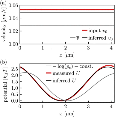 | ||
Fig. 5 (a) Inferred ν0 from driven experimental data compared to the desired input value ν0. Though there are some statistical deviations in the values for ν0 (related to Fig. 4(b)), both obtained values for ν0 are well distinguishable from the mean velocity ![[small nu, Greek, macron]](https://www.rsc.org/images/entities/i_char_e0ce.gif) (grey line). (b) The potential U(x) inferred from the driven data viaeqn (17) (black line) matches the potential measured from the equilibrium data projected on one period [0,L) using U(x) = −ln(peq(x)) − const. (red line) quite well. The barrier height (difference between minimum and maximum) is 2.76kBT in the red line and 2.65kBT in the black line, respectively. It deviates from − log(ps) (grey line) since the driven data set does not obey a Boltzmann density [see eqn (2) and (3)]. (grey line). (b) The potential U(x) inferred from the driven data viaeqn (17) (black line) matches the potential measured from the equilibrium data projected on one period [0,L) using U(x) = −ln(peq(x)) − const. (red line) quite well. The barrier height (difference between minimum and maximum) is 2.76kBT in the red line and 2.65kBT in the black line, respectively. It deviates from − log(ps) (grey line) since the driven data set does not obey a Boltzmann density [see eqn (2) and (3)]. | ||
4 Different notions of velocity
To provide more insight into the different notions of velocity in our system, we compute the bare velocity ν0, the drift velocity vdrift(x) in eqn (7), and the mean velocity![[small nu, Greek, macron]](https://www.rsc.org/images/entities/i_char_e0ce.gif) = 〈Xt − X0〉s/t in eqn (9) from the measured trajectories of the driven system. The results are shown in Fig. 6.
= 〈Xt − X0〉s/t in eqn (9) from the measured trajectories of the driven system. The results are shown in Fig. 6.
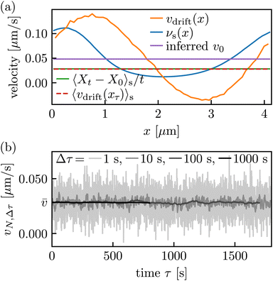 | ||
Fig. 6 (a) Different space-dependent and constant velocities in the NESS. See eqn (9) for different representations of the mean velocity ![[small nu, Greek, macron]](https://www.rsc.org/images/entities/i_char_e0ce.gif) . In equilibrium, only νdrift(x) deviates from zero. Quantities denoted by averages over xτ are independent of τ in the steady state and are here, for practical reasons to improve statistics, averaged over all τ ∈ [0,t]. (b) While . In equilibrium, only νdrift(x) deviates from zero. Quantities denoted by averages over xτ are independent of τ in the steady state and are here, for practical reasons to improve statistics, averaged over all τ ∈ [0,t]. (b) While ![[small nu, Greek, macron]](https://www.rsc.org/images/entities/i_char_e0ce.gif) = 〈xτ+Δτ−xτ〉s/Δτ for all τ and Δτ, see eqn (9), the approximation = 〈xτ+Δτ−xτ〉s/Δτ for all τ and Δτ, see eqn (9), the approximation  of this quantity over the finite number of trajectories N = 1168 as a function of τ, as expected, exhibits large fluctuations for small Δτ. of this quantity over the finite number of trajectories N = 1168 as a function of τ, as expected, exhibits large fluctuations for small Δτ. | ||
As mentioned above, two constants constitute a notion of velocity: the bare velocity ν0 and the mean velocity ![[small nu, Greek, macron]](https://www.rsc.org/images/entities/i_char_e0ce.gif) , see eqn (9). In addition, there are also local, x-dependent notions like the local mean velocity νs(x), as well as the drift velocity vdrift(x) = 〈dxt|xt = x〉/dt, see eqn (7). In equilibrium, only the drift velocity vdrift(x) deviates from 0. The mean velocity
, see eqn (9). In addition, there are also local, x-dependent notions like the local mean velocity νs(x), as well as the drift velocity vdrift(x) = 〈dxt|xt = x〉/dt, see eqn (7). In equilibrium, only the drift velocity vdrift(x) deviates from 0. The mean velocity ![[small nu, Greek, macron]](https://www.rsc.org/images/entities/i_char_e0ce.gif) can be computed in different ways; see eqn (9), some of which are also equivalent from a practical/numerical point of view (depending on how we choose to infer js). Note that generally, νs(x) ≠ 〈νs(xt)〉s ≠ vdrift(x) ≠ 〈vdrift(xt)〉s, that is, the different kinds of velocities indeed have a quite strikingly different meaning, which must be taken into account when characterizing and comparing transport properties.
can be computed in different ways; see eqn (9), some of which are also equivalent from a practical/numerical point of view (depending on how we choose to infer js). Note that generally, νs(x) ≠ 〈νs(xt)〉s ≠ vdrift(x) ≠ 〈vdrift(xt)〉s, that is, the different kinds of velocities indeed have a quite strikingly different meaning, which must be taken into account when characterizing and comparing transport properties.
5 First-passage times
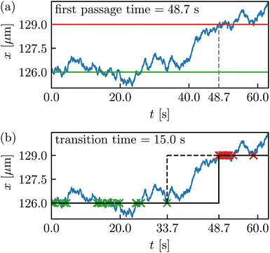
In this section, we evaluate the mean first-passage times, that is, the average time it takes for a particle to reach a certain point [see Fig. 7; in our case, the average time to cross the barrier in the potential U(x)] for the first time given some initial condition,61 using experimental data. The first-passage time for barrier crossing is an insightful observable, important, for instance, in the study of chemical reactions kinetics.77 Perhaps more important in the present context, first-passage observables are generally much more sensitive dynamics indicators than propagators, currents, or mean-squared particle displacement.8,63,64 As such, they are particularly suitable for critically assessing whether inferred properties of the dynamics (e.g., the parameters in the equations of motion) are appropriate. In particular, first-passage observables may distinguish between processes with identical transition probability densities,64 and, in contrast to mean-squared particle displacements, provide insight into the microscopic origin of anomalous dispersion in complex media.8,63Here we focus on two particular first-passage observables, namely the mean-first passage to transverse a distance equal to the period length L, 〈τ(x → x + L)〉 and the two-sided mean exit time from the interval [x − L,x + L], 〈τE(x ± L)〉. Note that we do not consider periodic boundary conditions here, i.e., we consider trajectories (Xτ)0≤τ≤t which evolve on the entire space and not only on [0,L). The chosen first-passage observables have two advantages. First, for a periodic potential U(x), they are independent of the initial position x,69 making them very practical to infer from experimental data. Second, the mean of its one-sided version, 〈τ(x → x + L)〉s is directly related to the mean velocity 〈τ(x → x + L)〉s = L/![[small nu, Greek, macron]](https://www.rsc.org/images/entities/i_char_e0ce.gif) , see eqn (9).
, see eqn (9).
To recapitulate where the independence comes from, consider τ(0 → L) and τ(x→x + L) for some x∈ [0,L]. Since we have one-dimensional trajectories, x is necessarily crossed in the transition 0 → L, and by the renewal theorem78,79 (note that we are dealing with a time-homogeneous Markov process with continuous paths) we immediately have statistical equality on the level of τ for τ(0 → L) = τ(0 → x) + τ(x → L). Moreover, by periodicity we obtain τ(0 → x) + τ(x → L) = τ(L → x + L) + τ(x → L) = τ(x → L) + τ(L → x + L) = τ(x → x + L), therefore τ(x → x + L) (and therefore 〈τ(x → x + L)〉) is independent of x, and similarly for τE(x ± L). We will exploit this in the notation and drop the dependence on x, i.e., 〈τ(x → x + L)〉 → 〈τ(L)〉.
The x-invariance helps to check the data for short-time bias due to under-sampling (see Appendix of ref. 8). Namely, whenever we infer τ from finite trajectories, say of duration t, starting at an arbitrary point x0, we estimate a conditional mean first-passage/exit time, 〈τ(L)|τ(L)<t〉,8i.e.,
 | (18) |
 is the probability density of τ(L), and the same holds for the two-sided exit time 〈τE(L)|τE(L) < t〉. Obviously,
  . For a periodic U(x) in the equilibrium setting ν0 = 0, 〈τ(L)〉 unlike the exit time 〈τE(L)〉 < ∞ is infinite, 〈τ(L)〉 = ∞ since the particle can escape to −∞ and thereby may not reach the target at any finite time. However, by the fundamental property of Brownian motion, in the equilibrium setting all trajectories eventually hit the target. Moreover, in the driven setting, we consider a bias towards the target, such that almost all trajectories reach the target in a finite time. Hence, we expect 〈τ(L)〉s < ∞61 (this would, of course, not be the case of a particle biased away from the target).
Any substantial deviations between the conditional and unconditioned first-passage (and exit times, respectively) reflect that a significant fraction of trajectories did not yet cross the barrier to the right of the initial condition and that the estimated mean first-passage time is statistically unreliable. The manifestation of this short-time bias in the equilibrium and driven setting is demonstrated in Fig. 8, where we mimic the effect of a progressively larger measurement time t in the experiment by disregarding long-time data. We find substantial effects of a finite duration of trajectories. In the equilibrium case, both the mean first-passage and the exit time increase with the duration t of trajectories, while in the driven case, the mean first-passage time is progressively approaching the predicted value. Based on the Langevin dynamics in eqn (2) or (3), the one-sided mean first-passage time (blue line) is known to diverge as t → ∞ in the equilibrium setting [see, e.g., ![[small nu, Greek, macron]](https://www.rsc.org/images/entities/i_char_e0ce.gif) → 0 in eqn (9)], while the two-sided version (orange line) must converge. In the non-equilibrium setting (green line), the mean first-passage time must converge, and we observe a quantitative agreement with the theoretical prediction L/
→ 0 in eqn (9)], while the two-sided version (orange line) must converge. In the non-equilibrium setting (green line), the mean first-passage time must converge, and we observe a quantitative agreement with the theoretical prediction L/![[small nu, Greek, macron]](https://www.rsc.org/images/entities/i_char_e0ce.gif) in eqn (9) (grey line), where the equality 〈τ(L)〉s = L/
in eqn (9) (grey line), where the equality 〈τ(L)〉s = L/![[small nu, Greek, macron]](https://www.rsc.org/images/entities/i_char_e0ce.gif) is approached for large t. If the deviation of the green and grey dashed line in Fig. 8(a), does not (approximately) vanish. We could immediately infer that the measurement time is too short. Equivalently, the fraction of successful trajectories (see Fig. 8(b)) ought to converge to 1 for the exit from the interval and generally for the driven setting (and asymptotically approach 1 for the one-sided first-passage in the equilibrium setting) if we are to infer a reliable estimate for 〈τ(L)〉. However, note that the additional test with the mean velocity
is approached for large t. If the deviation of the green and grey dashed line in Fig. 8(a), does not (approximately) vanish. We could immediately infer that the measurement time is too short. Equivalently, the fraction of successful trajectories (see Fig. 8(b)) ought to converge to 1 for the exit from the interval and generally for the driven setting (and asymptotically approach 1 for the one-sided first-passage in the equilibrium setting) if we are to infer a reliable estimate for 〈τ(L)〉. However, note that the additional test with the mean velocity ![[small nu, Greek, macron]](https://www.rsc.org/images/entities/i_char_e0ce.gif) may still be meaningful even if the fraction is already one (e.g., if one has a limited number of trajectories available or if one puts in the requirement of crossing the barrier as an additional condition).
may still be meaningful even if the fraction is already one (e.g., if one has a limited number of trajectories available or if one puts in the requirement of crossing the barrier as an additional condition).
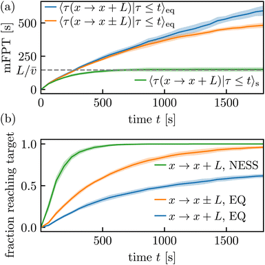 | ||
| Fig. 8 (a) Conditional mean first-passage times (mFPT) and (b) fraction of trajectories where the barrier crossing event was realized conditioned on times until t (i.e., we cut the data at time t to mimic shorter measurements). The green line approaches 148.8 s, which roughly agrees with the grey line at 146.4 s, confirming the last equality in eqn (9). Shaded regions show the sample standard deviation over the 11 (equilibrium “EQ”) or 13 (NESS) data sets. | ||
Note that a short-time bias is, in fact, typical. Specifically, whenever not (almost) all observed trajectories reach the target, the estimated mean first-passage time (or its inverse, the rate) will suffer from this bias. This occurs because the first-passage and the exit time are controlled (essentially dominated) by the long-time behaviour of  .61,80,81
6 Symmetry of transition-path times
An essential and closely related, but fundamentally quite different, concept to first-passage times is transition-path times.65–68,82 The transition-path time from a point A to a point B in (here considered in one-dimensional space) is defined as the time span between the last time that a trajectory (xτ)τ≥0 hits A before hitting B for the first time, see Fig. 7(b). This observable is deeply related to the concept of mile-stoning (see, e.g., ref. 68,83–86) and Fig. 7(b), (where the crosses indicate hits of the milestones). The important difference to first-passage times τ(A → B) is thus that the transition time
  does not contain the dwell time around A (see, e.g., ref. 68 for details). A practical difference for our analysis is that we had 0 or 1 samples per trajectory for the first-passage time (since we always started at t = 0) while a single trajectory may contain several transitions A → B and B → A, see Fig. 7. Moreover, we again consider the periodicity in space for the transition times.
Transition-path times encode subtle and important information about violations of the Markov property31,67,68 and are essential for consistent thermodynamics of non-Markovian processes.31,68,85,86 A particularly subtle, and at first glance surprising, property of transition-path times is the forward–backward symmetry for reversible Markov dynamics discovered in ref. 65 (for extensions, see ref. 32,68,87,88). It states that for a Markov process obeying detailed balance, we have the equality in time-distribution of transition paths,  . The surprising aspect is that if A is located in a potential minimum and B on a potential barrier, the duration of transition paths “uphill”' and “downhill” are statistically identical for any potential. Note that this symmetry does not hold for first-passage times (since the dwell times in A and B can be arbitrarily different).
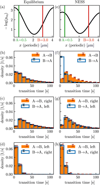
The transition-path time symmetry has seemingly not yet been experimentally verified (although its violations in multidimensional non-equilibrium systems have already been observed experimentally31 and by computer simulations88). Here we evaluate the transition times between two milestones (here points) A and B (see Fig. 9(a) and (e)) and evaluate frequency histograms of transition-path times as an estimator of their probability density for equilibrium (see Fig. 9(a)–(d)) and NESS dynamics (see Fig. 9(e)–(h)). Note that since the original transition-path time symmetry does not concern periodic systems, it only holds for transitions A → B and B → A either passing through the middle (around x = 2 μm) or passing through the periodic boundary (x = 0 μm), see overlap of blue and orange in Fig. 9(c) and (d), respectively. Note that the symmetry is equally expected to hold in one-dimensional NESS,87 as confirmed in Fig. 9(g) and (h) (it only breaks down in multidimensional NESS, see ref. 31). Nevertheless, we see in Fig. 9(b) that the symmetry also holds for “mixed”' transitions between A and B, i.e., if we consider all transitions indifferent to whether they do or do not make use of the periodic boundary. This is generally the case for periodic equilibrium dynamics (given 1d Markov) since orange and blue in Fig. 9(b) are a weighted average of orange and blue in Fig. 9(c) and (d) where both colours are weighted with the same proportions [different weights cannot occur in equilibrium since this would lead to a contraction as it implies directed motion (js ≠ 0)]. The symmetry is violated for mixed transitions in Fig. 9(f), since the weighting of Fig. 9(g) and (h) to obtain Fig. 9(f) is not the same for orange and blue.
To summarize, Fig. 9 demonstrates the validity of the predicted transition-path time symmetry between two milestones (Fig. 9(c), (d), (g) and (h)). While the transition-path time symmetry does not apply to periodic NESS dynamics (Fig. 9(f)), it holds true (in addition to the “unmixed” transitions in Fig. 9(c), (d), (g) and (h)) for periodic equilibrium dynamics (Fig. 9(b)).
7 Conclusions
We interrogated path-wise properties of driven colloids in a periodic light field to experimentally demonstrate some highly intricate and insightful features of transport, kinetics, and transition-path time statistics out of equilibrium. Our main goal was to emphasize how these observables can be systematically utilized to critically assess and verify the quality of the experimental data. We have reiterated that, with sufficient control and sampling, even subtle theoretical predictions can be rigorously tested and quantitatively validated. We hope this will motivate the experimental soft-matter community to undertake such tests and further enhance the quality of experimental data.Beyond the previous analyses of first-passage observables in experimental data8,28 we compared the mean particle velocity with the corresponding first-passage result69 to check for short-time biases in non-equilibrium steady states. Despite the measurement time being long enough for trajectories to equilibrate within one period [0,L), we illustrate that observables, such as the one-sided mean first-passage time in equilibrium, (have not yet converged, highlighting the intricate features of first-passage times and more generally, path-based observables). That is, small statistical fluctuations (i.e., small error bars) do not necessarily imply a sufficient quality of data as exemplified by the short-time biases in Fig. 8. From a practical perspective, our results show that first-passage analysis can be used to systematically test experimental data for short-time biases.
Moreover, we verify and extend predicted symmetries for the more subtle transition-path times. By showing that the symmetry persists in effectively one-dimensional non-equilibrium systems, we underscore the usefulness of violations of the transition-path-time symmetry to infer simultaneously broken time-reversal symmetry and the presence of multiple transition pathways.31,87
We also highlighted two well-established but distinct, yet mathematically equivalent, formulations of the Langevin equation of motion for colloidal particles. Notably, the second formulation, while less commonly employed in experiments, provides a more thermodynamically expressive framework. We hope this will encourage further integration between soft-matter experiments and stochastic thermodynamics, particularly in advancing thermodynamic inference using speed limits and thermodynamic uncertainty relations.
Author contributions
AG and SUE conceptualized the project, MAES and AG were responsible for the administration. SUE and AG provided the resources and acquired the funding for the experimental and theoretical work, respectively. CD and AG developed the theory. CD, YM, ABZB and MAES performed the investigations and validation. MAES and CD developed the software. ABZB and YM worked on the experimental setup. YM, CD and MAES worked on the methodology, data curation, and visualization. CD and AG wrote the original draft. CD, AG, ABZB, YM and MAES reviewed and edited the final version of the manuscript.Data availability
Data for this article, including all particle trajectories analyzed in the manuscript, are available at Zenodo at https://doi.org/10.5281/zenodo.13908799.Conflicts of interest
There are no conflicts to declare.Appendix
Details on the periodic potential
For the above analysis, we determined period L by comparing histograms for xτ ≡ Xτ![[thin space (1/6-em)]](https://www.rsc.org/images/entities/char_2009.gif) mod
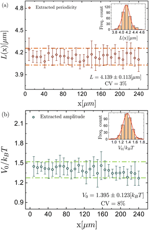
mod![[thin space (1/6-em)]](https://www.rsc.org/images/entities/char_2009.gif) L over the left and right half, respectively, of particles in the field of view. The chosen value correct value of L was optimized such that the two histograms optimally agree. While this does not rely on any assumptions about the exact shape of the potential (the shape was only later inferred from histograms; we only assumed that there is one barrier per period to remove ambiguity, since any L-periodic system is, e.g., also 2L-periodic), this procedure may generally only serve as a fine-tuning for the value for L. Therefore, we here also present an alternative, more systematic, approach to infer L using an approximation for the shape of U(x). Moreover, while the theory and inference of U(x) in the main part of the paper address general periodic potentials, the experimentally realized U(x) is well approximated by a cosine. To elaborate on the discussion of the inference of U(x), and to show the spatial variation that is not investigated in the paper (since it is lost after projecting onto one period; as done, e.g., to arrive at Fig. 5(b)), in this Appendix we also show a complementary approach, where we assume a cosine-shape and infer the amplitude and its spatial variation. Following earlier experiments with comparable setups, we assume that the effective potential induced by the periodic light field can be well approximated by,2,70U(x) = U0cos(kx) + Ubg, with k = 2π/L, U0 the potential amplitude and Ubg a constant background contribution. The potential background Ubg becomes irrelevant as it is neglected by the derivative in eqn (1). Over the whole field of view, particle density profiles ρ(x) for the equilibrium trajectories were analyzed to extract the periodicity and amplitude of an underlying potential via ρ(x) ∝ exp[−U(x)/kBT]. The natural logarithm of the density, ln(ρ(x)), was evaluated, and its derivative,
L over the left and right half, respectively, of particles in the field of view. The chosen value correct value of L was optimized such that the two histograms optimally agree. While this does not rely on any assumptions about the exact shape of the potential (the shape was only later inferred from histograms; we only assumed that there is one barrier per period to remove ambiguity, since any L-periodic system is, e.g., also 2L-periodic), this procedure may generally only serve as a fine-tuning for the value for L. Therefore, we here also present an alternative, more systematic, approach to infer L using an approximation for the shape of U(x). Moreover, while the theory and inference of U(x) in the main part of the paper address general periodic potentials, the experimentally realized U(x) is well approximated by a cosine. To elaborate on the discussion of the inference of U(x), and to show the spatial variation that is not investigated in the paper (since it is lost after projecting onto one period; as done, e.g., to arrive at Fig. 5(b)), in this Appendix we also show a complementary approach, where we assume a cosine-shape and infer the amplitude and its spatial variation. Following earlier experiments with comparable setups, we assume that the effective potential induced by the periodic light field can be well approximated by,2,70U(x) = U0cos(kx) + Ubg, with k = 2π/L, U0 the potential amplitude and Ubg a constant background contribution. The potential background Ubg becomes irrelevant as it is neglected by the derivative in eqn (1). Over the whole field of view, particle density profiles ρ(x) for the equilibrium trajectories were analyzed to extract the periodicity and amplitude of an underlying potential via ρ(x) ∝ exp[−U(x)/kBT]. The natural logarithm of the density, ln(ρ(x)), was evaluated, and its derivative,  , to remove any background contributions. We used a sinusoidal function to fit the derivative for a window consisting of two periods and performed the same analysis for the entire dataset, covering 30 windows. Averaging the results across all windows we estimate the periodicity and potential amplitude of the light field. The insets in Fig. 10 show histograms of the periodicity and amplitude values, with the frequency count plotted versus the extracted periodicity and amplitude for all measurements. The red curve represents a Gaussian fit to the histogram. This allows for a statistical summary with the mean and standard deviation extracted from the fit, and in particular shows the spatial variation. The error bars in the plot represent the standard deviation of the extracted periodicity values within each window. The results of the inference of L in Fig. 10(a), based on approximating U as a cosine, are in excellent agreement with the value L = 4.135 μm chosen in the main part by matching histograms in different parts in the field of view without assuming the shape of U(x). Moreover, the amplitude inferred in Fig. 10(b) match closely with the barrier heights of 2.76kBT and 2.65kBT in Fig. 5(b), keeping in mind that the barrier (difference of maximum and minimum) in the cosine potential is 2V0.
Acknowledgements
Financial support from the European Research Council (ERC) under the European Unions Horizon Europe research and innovation program (grant agreement no. 101086182 to AG) and from the Deutsche Forschungsgemeinschaft (DFG), project number 459399860 (to SUE and MAES), is gratefully acknowledged. This work is dedicated to the memory of our friend, mentor and colleague, Stefan U. Egelhaaf. Open Access funding provided by the Max Planck Society.Notes and references
- H. Löwen, J. Phys.: Condens. Matter, 2008, 20, 404201 CrossRef.
- F. Evers, R. D. L. Hanes, C. Zunke, R. F. Capellmann, J. Bewerunge, C. Dalle-Ferrier, M. C. Jenkins, I. Ladadwa, A. Heuer and R. Castañeda-Priego, et al. , Eur. Phys. J.-Spec. Top., 2013, 222, 2995 CrossRef.
- G. Volpe, G. Volpe and S. Gigan, Sci. Rep., 2014, 4, 3936 CrossRef PubMed.
- A. Ashkin, Proc. Natl. Acad. Sci. U. S. A., 1997, 94, 4853 CrossRef CAS PubMed.
- D. G. Grier, Nature, 2003, 424, 810 CrossRef CAS PubMed.
- I. A. Martínez, É. Roldán, L. Dinis, D. Petrov, J. M. R. Parrondo and R. A. Rica, Nat. Phys., 2015, 12, 67 Search PubMed.
- A. Militaru, A. Lasanta, M. Frimmer, L. L. Bonilla, L. Novotny and R. A. Rica, Phys. Rev. Lett., 2021, 127, 130603 CrossRef CAS PubMed.
- C. Zunke, J. Bewerunge, F. Platten, S. U. Egelhaaf and A. Godec, Sci. Adv., 2022, 8, eabk0627 CrossRef CAS PubMed.
- S. A. M. Loos, S. Monter, F. Ginot and C. Bechinger, Phys. Rev. X, 2024, 14, 021032 CAS.
- M. Ibáñez, C. Dieball, A. Lasanta, A. Godec and R. A. Rica, Nat. Phys., 2024, 20, 135 Search PubMed.
- I. A. Martínez, E. Roldán, L. Dinis and R. A. Rica, Soft Matter, 2017, 13, 22 RSC.
- V. Blickle and C. Bechinger, Nat. Phys., 2011, 8, 143 Search PubMed.
- N. Osterman, I. Poberaj, J. Dobnikar, D. Frenkel, P. Ziherl and D. Babic, Phys. Rev. Lett., 2009, 103, 228301 CrossRef CAS PubMed.
- R. M. Erb, H. S. Son, B. Samanta, V. M. Rotello and B. B. Yellen, Nature, 2009, 457, 999 CrossRef CAS PubMed.
- A. Yethiraj, Soft Matter, 2007, 3, 1099 RSC.
- A. Terray, J. Oakey and D. W. M. Marr, Science, 2002, 296, 1841 Search PubMed.
- J. K. G. Dhont, An introduction to dynamics of colloids, Elsevier, 1996 Search PubMed.
- A. J. Banchio, J. Bergenholtz and G. Nägele, Phys. Rev. Lett., 1999, 82, 1792–1795 CrossRef CAS.
- H. Löwen, Dynamical Density Functional Theory for Brownian Dynamics of Colloidal Particles, Springer, Singapore, 2016, pp. 255–284 Search PubMed.
- R. Wittkowski and H. Löwen, Mol. Phys., 2011, 109, 2935–2943 CrossRef CAS.
- K. Sekimoto, Stochastic Energetics, Springer, Berlin Heidelberg, 2010 Search PubMed.
- U. Seifert, Rep. Prog. Phys., 2012, 75, 126001 CrossRef PubMed.
- G. M. Wang, E. M. Sevick, E. Mittag, D. J. Searles and D. J. Evans, Phys. Rev. Lett., 2002, 89, 050601 CrossRef CAS PubMed.
- A. Imparato, L. Peliti, G. Pesce, G. Rusciano and A. Sasso, Phys. Rev. E: Stat., Nonlinear, Soft Matter Phys., 2007, 76, 050101 CrossRef CAS PubMed.
- G. M. Wang, J. C. Reid, D. M. Carberry, D. R. M. Williams, E. M. Sevick and D. J. Evans, Phys. Rev. E: Stat., Nonlinear, Soft Matter Phys., 2005, 71, 046142 CrossRef CAS PubMed.
- D. M. Carberry, J. C. Reid, G. M. Wang, E. M. Sevick, D. J. Searles and D. J. Evans, Phys. Rev. Lett., 2004, 92, 140601 CrossRef CAS PubMed.
- A. Magazzù, A. Callegari, J. P. Staforelli, A. Gambassi, S. Dietrich and G. Volpe, Soft Matter, 2019, 15, 2152–2162 RSC.
- A. L. Thorneywork, J. Gladrow, Y. Qing, M. Rico-Pasto, F. Ritort, H. Bayley, A. B. Kolomeisky and U. F. Keyser, Sci. Adv., 2020, 6, eaaz4642 CrossRef CAS PubMed.
- N. Zijlstra, D. Nettels, R. Satija, D. E. Makarov and B. Schuler, Phys. Rev. Lett., 2020, 125, 146001 CrossRef CAS PubMed.
- K. Neupane, D. B. Ritchie, H. Yu, D. A. N. Foster, F. Wang and M. T. Woodside, Phys. Rev. Lett., 2012, 109, 068102 CrossRef PubMed.
- J. Gladrow, M. Ribezzi-Crivellari, F. Ritort and U. F. Keyser, Nat. Commun., 2019, 10, 55 CrossRef CAS PubMed.
- R. Satija, A. M. Berezhkovskii and D. E. Makarov, Proc. Natl. Acad. Sci. U. S. A., 2020, 117, 27116–27123 CrossRef CAS PubMed.
- F. Sturzenegger, F. Zosel, E. D. Holmstrom, K. J. Buholzer, D. E. Makarov, D. Nettels and B. Schuler, Nat. Commun., 2018, 9, 4708 CrossRef PubMed.
- S. N. Majumdar and A. Comtet, Phys. Rev. Lett., 2002, 89, 060601 CrossRef PubMed.
- G. Bel and E. Barkai, Phys. Rev. Lett., 2005, 94, 240602 CrossRef.
- A. Rebenshtok and E. Barkai, J. Stat. Phys., 2008, 133, 565 CrossRef.
- S. Sabhapandit, S. N. Majumdar and A. Comtet, Phys. Rev. E: Stat., Nonlinear, Soft Matter Phys., 2006, 73, 051102 CrossRef PubMed.
- A. Lapolla, D. Hartich and A. Godec, Phys. Rev. Res., 2020, 2, 043084 CrossRef CAS.
- C. Dieball and A. Godec, Phys. Rev. Lett., 2022, 129, 140601 CrossRef CAS PubMed.
- C. Dieball and A. Godec, Phys. Rev. Res., 2022, 4, 033243 CrossRef CAS.
- M. Baiesi, C. Maes and B. Wynants, Phys. Rev. Lett., 2009, 103, 010602 CrossRef PubMed.
- A. Dechant and S.-i Sasa, Proc. Natl. Acad. Sci. U. S. A., 2020, 117, 6430 CrossRef CAS PubMed.
- N. Shiraishi, K. Funo and K. Saito, Phys. Rev. Lett., 2018, 121, 070601 Search PubMed.
- V. T. Vo, T. Van Vu and Y. Hasegawa, Phys. Rev. E, 2020, 102, 062132 CrossRef CAS PubMed.
- T. Van Vu and K. Saito, Phys. Rev. X, 2023, 13, 011013 CAS.
- C. Dieball and A. Godec, Phys. Rev. Lett., 2024, 133, 067101 CrossRef CAS PubMed.
- A. C. Barato and U. Seifert, Phys. Rev. Lett., 2015, 114, 158101 CrossRef PubMed.
- J. M. Horowitz and T. R. Gingrich, Nat. Phys., 2019, 16, 15 Search PubMed.
- K. Macieszczak, K. Brandner and J. P. Garrahan, Phys. Rev. Lett., 2018, 121, 130601 CrossRef CAS PubMed.
- T. Koyuk and U. Seifert, Phys. Rev. Lett., 2019, 122, 230601 CrossRef CAS PubMed.
- T. Koyuk and U. Seifert, Phys. Rev. Lett., 2020, 125, 260604 CrossRef CAS PubMed.
- A. Dechant and S.-i Sasa, Phys. Rev. X, 2021, 11, 041061 CAS.
- G. Falasco and M. Esposito, Phys. Rev. Lett., 2020, 125, 120604 CrossRef CAS PubMed.
- R.-S. Fu and T. R. Gingrich, Phys. Rev. E, 2022, 106, 024128 CrossRef CAS PubMed.
- T. Koyuk and U. Seifert, Phys. Rev. Lett., 2022, 129, 210603 CrossRef CAS PubMed.
- C. Dieball and A. Godec, Phys. Rev. Lett., 2023, 130, 087101 CrossRef CAS PubMed.
- R. Cerbino and V. Trappe, Phys. Rev. Lett., 2008, 100, 188102 CrossRef PubMed.
- M. A. Kamal, M. Brizioli, T. Zinn, T. Narayanan, R. Cerbino, F. Giavazzi and A. Pal, J. Colloid Interface Sci., 2024, 660, 314–320 CrossRef CAS PubMed.
- F. Giavazzi and R. Cerbino, J. Opt., 2014, 16, 083001 CrossRef.
- M. A. Escobedo-Sánchez, J. P. Segovia-Gutiérrez, A. B. Zuccolotto-Bernez, J. Hansen, C. C. Marciniak, K. Sachowsky, F. Platten and S. U. Egelhaaf, Soft Matter, 2018, 14, 7016–7025 RSC.
- S. Redner, A Guide to First-Passage Processes, Cambridge University Press, 2001 Search PubMed.
- R. Metzler, G. Oshanin and S. Redner, First-Passage Phenomena and Their Applications, World Scientific, 2013 Search PubMed.
- S. Condamin, V. Tejedor, R. Voituriez, O. Bénichou and J. Klafter, Proc. Natl. Acad. Sci. U. S. A., 2008, 105, 5675 CrossRef CAS PubMed.
- Y. Meroz, I. M. Sokolov and J. Klafter, Phys. Rev. Lett., 2011, 107, 260601 CrossRef PubMed.
- A. M. Berezhkovskii, G. Hummer and S. M. Bezrukov, Phys. Rev. Lett., 2006, 97, 020601 CrossRef PubMed.
- R. Satija, A. M. Berezhkovskii and D. E. Makarov, Proc. Natl. Acad. Sci. U. S. A., 2020, 117, 27116–27123 CrossRef CAS PubMed.
- A. M. Berezhkovskii and D. E. Makarov, J. Phys. Chem. Lett., 2018, 9, 2190–2195 CrossRef CAS PubMed.
- D. Hartich and A. Godec, Phys. Rev. X, 2021, 11, 041047 CAS.
- P. Reimann, C. Van den Broeck, H. Linke, P. Hänggi, J. M. Rubi and A. Pérez-Madrid, Phys. Rev. Lett., 2001, 87, 010602 CrossRef CAS PubMed.
- R. F. Capellmann, J. Bewerunge, F. Platten and S. U. Egelhaaf, Rev. Sci. Instrum., 2017, 88, 056102 CrossRef CAS PubMed.
- D. Blair and E. Dufresne, The Matlab Particle Tracking Code Repository, https://site.physics.georgetown.edu/matlab/, visited on 21/01/20.
- X. Michalet, Phys. Rev. E: Stat., Nonlinear, Soft Matter Phys., 2010, 82, 041914 CrossRef PubMed.
- C. W. Gardiner, Handbook of Stochastic Methods for Physics, Chemistry, and the Natural Sciences, Springer-Verlag, Berlin New York, 2nd edn, 1985 Search PubMed.
- H. Risken, The Fokker–Planck Equation, Springer, Berlin Heidelberg, 1989 Search PubMed.
- A. Chowdhury, F. Wood and B. J. Ackerson, Opt. Commun., 1991, 86, 547–554 CrossRef.
- J. Bewerunge and S. U. Egelhaaf, Phys. Rev. Accel. Beams, 2016, 93, 013806 Search PubMed.
- P. Hänggi, P. Talkner and M. Borkovec, Rev. Mod. Phys., 1990, 62, 251–341 CrossRef.
- A. J. F. Siegert, Phys. Rev., 1951, 81, 617–623 CrossRef.
- J. Keilson, J. Appl. Probab., 1965, 2, 405–428 CrossRef.
- O. Bénichou, C. Chevalier, J. Klafter, B. Meyer and R. Voituriez, Nat. Chem., 2010, 2, 472 CrossRef PubMed.
- A. Godec and R. Metzler, Phys. Rev. X, 2016, 6, 041037 Search PubMed.
- A. Godec and D. E. Makarov, J. Phys. Chem. Lett., 2023, 14, 49–56 CrossRef CAS PubMed.
- J. M. Bello-Rivas and R. Elber, J. Chem. Phys., 2015, 142, 094102 CrossRef PubMed.
- C. Schütte, F. Noé, J. Lu, M. Sarich and E. Vanden-Eijnden, J. Chem. Phys., 2011, 134, 204105 CrossRef PubMed.
- D. Hartich and A. Godec, Phys. Rev. Res., 2023, 5, L032017 CrossRef CAS.
- K. Blom, K. Song, E. Vouga, A. Godec and D. E. Makarov, Proc. Natl. Acad. Sci. U. S. A., 2024, 121, e2318333121 CrossRef CAS PubMed.
- A. M. Berezhkovskii and D. E. Makarov, J. Chem. Phys., 2019, 151, 065102 CrossRef.
- A. Ryabov, D. Lips and P. Maass, J. Phys. Chem. C, 2019, 123, 5714–5720 CrossRef CAS.
| This journal is © The Royal Society of Chemistry 2025 |

