Predicting self-assembly of sequence-controlled copolymers with stochastic sequence variation

Abstract

Sequence-controlled copolymers can self-assemble into a wide assortment of complex architectures, with exciting applications in nanofabrication and personalized medicine. However, polymer synthesis is notoriously imprecise, and stochasticity in both chemical synthesis and self-assembly poses a significant challenge to tight control over these systems. While it is increasingly viable to design “protein-like” sequences, specifying each individual monomer in a chain, the effect of variability within those sequences has not been well studied. In this work, we performed nearly 15 000 molecular dynamics simulations of sequence-controlled copolymer aggregates with varying level of sequence stochasticity. We utilized unsupervised learning to characterize the resulting morphologies and found that sequence variation leads to relatively smooth and predictable changes in morphology compared to ensembles of identical chains. Furthermore, structural response to sequence variation was accurately modeled using supervised learning, revealing several interesting trends in how specific families of sequences break down as monomer sequences become more variable. Our work presents a way forward in understanding and controlling the effect of sequence variation in sequence-controlled copolymer systems, which can hopefully be used to design advanced copolymer systems for technological applications in the future.

---

1 Introduction

Block copolymers consist of two or more polymer chains attached at their ends.¹ In dilute solution, these macromolecules have been shown to self-assemble into an assortment of nontrivial architectures,^2,3 with applications in drug delivery and personalized medicine.^4–7 The character of this self-assembly hinges upon the sequence of constituent blocks, resulting in a vast spectrum of possible morphologies, including micelles,^8,9 strings or wires,¹⁰ and vesicles.¹¹

In this vein, there has been increasing interest in sequence-controlled or protein-like copolymers as their aggregation behavior can be carefully tuned. The design of single-chain aggregation has been studied for more than 20 years,¹² with modern design methods assisting in both accelerating and broadening the search.^13–16 Some recent efforts have also been directed toward melts or aggregates of sequence-controlled copolymers,^17–19 though this remains somewhat less prevalent compared to studies of single chains. In our own prior work,^20,21 we studied the self-assembly of a model sequence-controlled copolymer into a large variety of different aggregate structures and showed that changing even a single monomer in a 20-mer may significantly alter the self-assembled morphology.

While the range of possible morphologies is known, it is challenging to obtain highly sequence-controlled polymers in practice. Chain growth polymerization is statistical in nature and provides imprecise control over the final sequence.²² Some causes of this are side reactions, such as chain transfer and radical coupling, which can be unavoidable. Reversible-deactivation radical polymerization techniques have been shown to generate more accurate sequences, especially in recent years, but they, too, cannot achieve perfect accuracy.²³ Some recent developments in synthesis have yielded new levels of sequence control,^24–29 but exact control over every monomer in the system still seems unlikely.

Since experimentally synthesized polymers are imperfect (i.e., not identical in length and monomer sequence) due to this inherent randomness in chain synthesis and self-assembly, the polymers community has invested some effort in developing descriptions that account for such variability. One example is BigSMILES,³⁰ an extension of the popular SMILES notation³¹ for chemical structure. BigSMILES supports “stochastic objects” such as side chains or repeat units that vary statistically due to polymerization chemistry. These stochastic objects are machine-friendly representations of the natural variations in polymer sequences (or, more generally, structures) and allow the encoding of ensembles of similar molecular structures that vary in random but well-behaved ways.

In this work, we extend our previous investigation^20,21 to monodisperse (a term we reserve for describing chain length) but non-identical (stochastic) chains, such that each aggregate contains an ensemble of similar sequences derived from a common “template” sequence. We use the term template to refer to the intended or as-designed monomer sequence to clarify that the monomer sequence within each chain in the simulation may vary from that template copolymer. This variation results in an ensemble of monodisperse 20-mers (as in our previous work) whose monomer sequence (and composition) vary in prescribed ways.

The self-assembly of these chains with stochastically varying monomer sequences fundamentally differs from that of either a single chain or ensembles of identical sequence-controlled copolymers, as in our prior work. These stochastic variations pose even greater challenges to conventional methods for modeling macromolecular aggregation such as self-consistent field theory (SCFT),^32–36 which cannot account for stochastic sequence variation at the monomer level, especially monomer-level sequence variation within one simulation. Our previous work²¹ demonstrated the predictive capability of data-driven models to rapidly screen from over 60 000 possible monomer sequences to identify the desired morphology. This framework significantly reduces the computational demands previously required for sequence-controlled polymer design. However, our prior work and others^17–19 used simulations of perfectly monodisperse and identical polymer chains within the system (all chains of identical length and monomer sequences), which limits their translation to presently available synthesis techniques.²⁸

We simulate the self-assembly of ensembles of sequence-controlled copolymers with stochastic sequence variation using molecular dynamics (MD), a scenario that has received little attention in the published literature. To this end, we generated a large dataset of different template sequences under varying levels of sequence variability, yielding nearly 15 000 simulation trajectories. These trajectories were analyzed with our previously established dimensionality reduction technique,²⁰ providing new insight into how these variations in monomer sequence affect the self-assembled morphologies. We also applied supervised learning to model the effect of stochastic sequence variation as a function of template morphology and degree of stochasticity. Our model's prediction error when deployed on unseen test data was comparable to the intrinsic uncertainty resulting from the self-assembly process, indicating excellent performance. Finally, we used this model to quantitatively describe the sensitivity of different self-assembled morphologies to sequence variation.

2 Methods

2.1 Molecular dynamics simulations

We follow the same simulation procedures as in ref. 20. Each coarse-grained polymer chain contains a sequence of A and B beads, with the A beads being attractive and the B beads being purely repulsive. The attractive beads interact with each other using the Lennard-Jones potential³⁷ (σ, ε, r_cut = 3σ), while the purely repulsive beads' self- and cross-interactions are described using the Weeks–Chandler–Anderson potential (σ, ε, r_cut = 2^1/6σ).³⁸ Here the σ is the dimensionless bead diameter and ε is the dimensionless energy unit. The bonds between beads in the chain were described by the standard finitely extensible nonlinear elastic potential³⁹ . An implicit solvent model was used to maximize computational efficiency, so solvent interactions were neglected. All simulations were performed using the HOOMD-blue⁴⁰ simulation package with an NVT ensemble and a Langevin thermostat at fixed temperature T = 0.5ε with damping constant γ = 0.1. The density is fixed at ρ = 0.05m/σ³, with the box size set to L ≈ 40σ on each side and the simulation containing 500 chains of length L = 20/σ. Simulations were run at a time step of δt = 0.005τ, and the aggregates were allowed to equilibrate for 5 × 10⁶ timesteps (2.5 × 10⁴τ).

Our previous work^20,21 was limited to completely identical, monodisperse chains. Here, in contrast, stochasticity was introduced by allowing each monomer bead from each template sequence in the simulation to randomly (and independently) flip at a fixed probability p (Fig. 1a). Sequences were independently randomized, giving up to 500 unique sequences (although some independent randomization may coincidentally result in the same sequence). Note that these events resulted in a random selection between A and B type such that p = 1 generated completely random sequences (if p is defined as the probability of changing type then p = 1 would simply yield the sequence with all A replaced by B and vice versa). By defining p as a probability for a bead to flip if and only if the bead succeeds on a coin flip, we avoid having the inverse sequences at p = 1. The inherent stochasticity observed in the self-assembly process^20,21 was investigated by creating five replicas of each set of input parameters (i.e., template sequence and p).

Fig. 1 Schematic describing the supervised learning method used to predict the final manifold coordinates (Z) of a template sequence (Z°) that has undergone some amount of sequence variation (p). (a) illustrating the probability of a bead to switch types, where every bead is given a random number from 0 to 1, and beads with a random number less than or equal to the chosen p value are given a 50% chance to flip their type. (b) Showing the predicted trajectory of a starting sequence on the manifold as randomness is increased.

The relationship between our p parameter and real-world copolymer systems deserves some consideration. Experimental systems with well-defined reactivity ratios might exhibit some characteristic p, but this would result in variations in monomer sequences, whereas our coarse-grained model has variations in groups of monomers (multiple monomers making up each bead). Also, our coarse-grained system assumes no selectivity in the reaction, which makes the behavior a bit simpler. These effects could be represented within a similar coarse-grained model through additional bead types representing blends of monomer units in different ratios and consequently incorporating a matrix of transition probabilities that depend on the base sequence. We leave this additional complexity to future study, but felt the need to clarify these aspects for the sake of the reader.

2.2 Unsupervised representation learning

The same unsupervised learning method discussed in our previous work²⁰ was used to generate the Z order parameters from the simulation trajectories. To summarize, the beads are first further coarse-grained such that 10 beads are represented by a single point at their center of mass. These coarsened point clouds are used to generate geometric features of the local environments according to ref. 41. The uniform manifold approximation and projection (UMAP)⁴² technique is then applied to project these local features into a 3D coordinate space; we refer to this as the local UMAP. These local features are pooled into a global feature for the entire simulation snapshot by generating a 3D histogram of all the local coordinates, similar to kernel density estimation. Finally, this histogram is used to embed the snapshot into a 2D space with a second UMAP; we refer to this as the global UMAP. All aspects of this embedding process are identical to ref. 20, and the source code is available on Github.⁴³ All relevant code and data are also available in a Zenodo repository created for this project.⁴⁴

2.3 Supervised learning

Once the Z order parameter was obtained for each sequence, we randomly split the dataset into training (60%), validation (20%), and testing (20%) sets using scikit-learn.⁴⁵ These splits were performed on sequences rather than individual observations to avoid data leakage (e.g., the same sequence appearing in training and test sets does not provide an accurate view of generalization performance). Next, a shallow Neural Network (NN) was trained to approximate the function,where Z° represents the order parameter for a template sequence (i.e., p = 0), p is the level of mutation applied, and Z is the model prediction at that p (Fig. 1b). Note that this NN is separate from the previously defined unsupervised learning task. The NN model was implemented in pytorch⁴⁶ and the hyperparameters were tuned with Bayesian optimization using ax-platform⁴⁷ (the optimized hyperparameters are reported in the results section).

2.4 Sensitivity analysis

After the model was trained, the sensitivity S of Z to changes in p was calculated according to the L₂ norm of the gradient at various points (Z°, p) throughout the manifold, i.e.,The model was also evaluated for any spatial error dependence, specifically whether manifold location correlates to certain errors. This was done by applying the model to the training, testing, and validation datasets and finding the Euclidean distance between the predicted manifold location and the simulated manifold location.

3 Results

3.1 Molecular dynamics simulations

We simulated 259 randomly selected, 20-monomer-long sequences at 11 p values ranging from 0 to 1 with five replicas each for a total of 14 795 total MD trajectories. The natural variability in MD simulations and the randomization of the sequences resulted in differences in the Z order parameter for identical runs. Across all p values, the Root Mean Square Deviation (RMSD) for these Z order parameters averaged to be 1.07, with no spatial dependence on RMSD throughout the manifold, as seen in Fig. 3. To visualize the space of possible morphologies, including strings, spherical micelles, membranes, liquids, vesicles, wormlike micelles, and structured liquids as observed in ref. 20, we render selected snapshots in Fig. 2 to form an approximately regular grid. Beyond the recognizable structures, we observed continuous variations of each morphology, with no apparent discontinuities in the order parameter space; thus, many aggregates for which we have no obvious name are shown. Only snapshots for p = 0 are shown in Fig. 2 for consistency with our prior work. The full dataset, including gsd simulation trajectories and full-resolution renderings in png format, are available in our Zenodo archive.⁴⁴

Fig. 2 A representative subset of the 14 795 total simulations performed for this work as embedded in the manifold generated in ref. 20. The color scheme is the same as the one introduced there, with each bead being colored in RGB space according to its position in the local environment manifold.

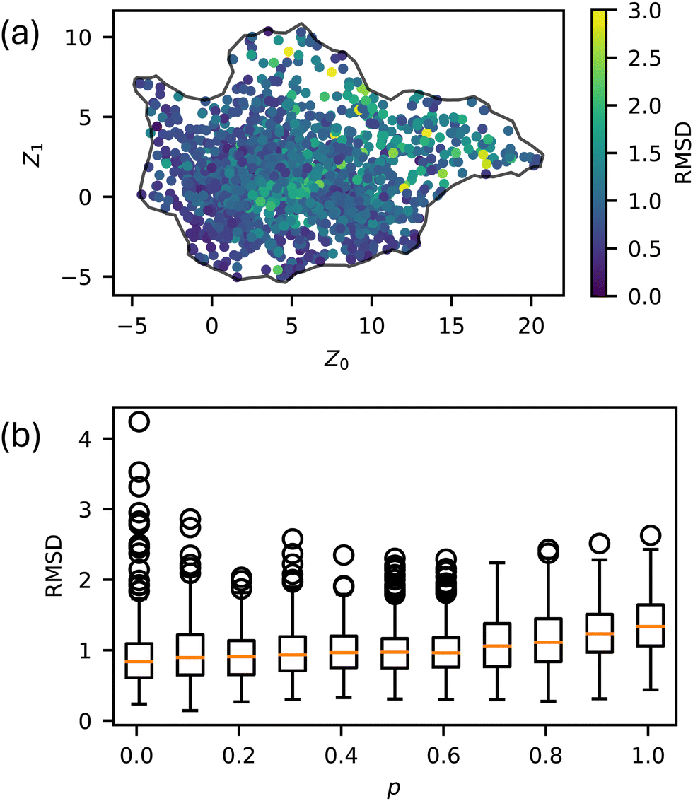Fig. 3 Natural variability of Z order parameters throughout the latent space. (a) RMSD for each sequence at each p value, and (b) RMSD as a function of p.

When introducing stochastic sequences (i.e., p > 0), we find that morphologies tend towards a center point, which we refer to as Z^R ≈ (5,1). Such a point must exist because when p = 1, all sequences are equivalent (completely random). This behavior is illustrated for some representative sequences in Fig. 4; we choose sequences for which Z° are on the periphery of the manifold to best illustrate their breakdown from “archetypal” morphologies into the common random morphology. As discussed in our prior work, Z^R must be located in the center of the manifold to maximize the distance from the recognizable structures around the periphery.

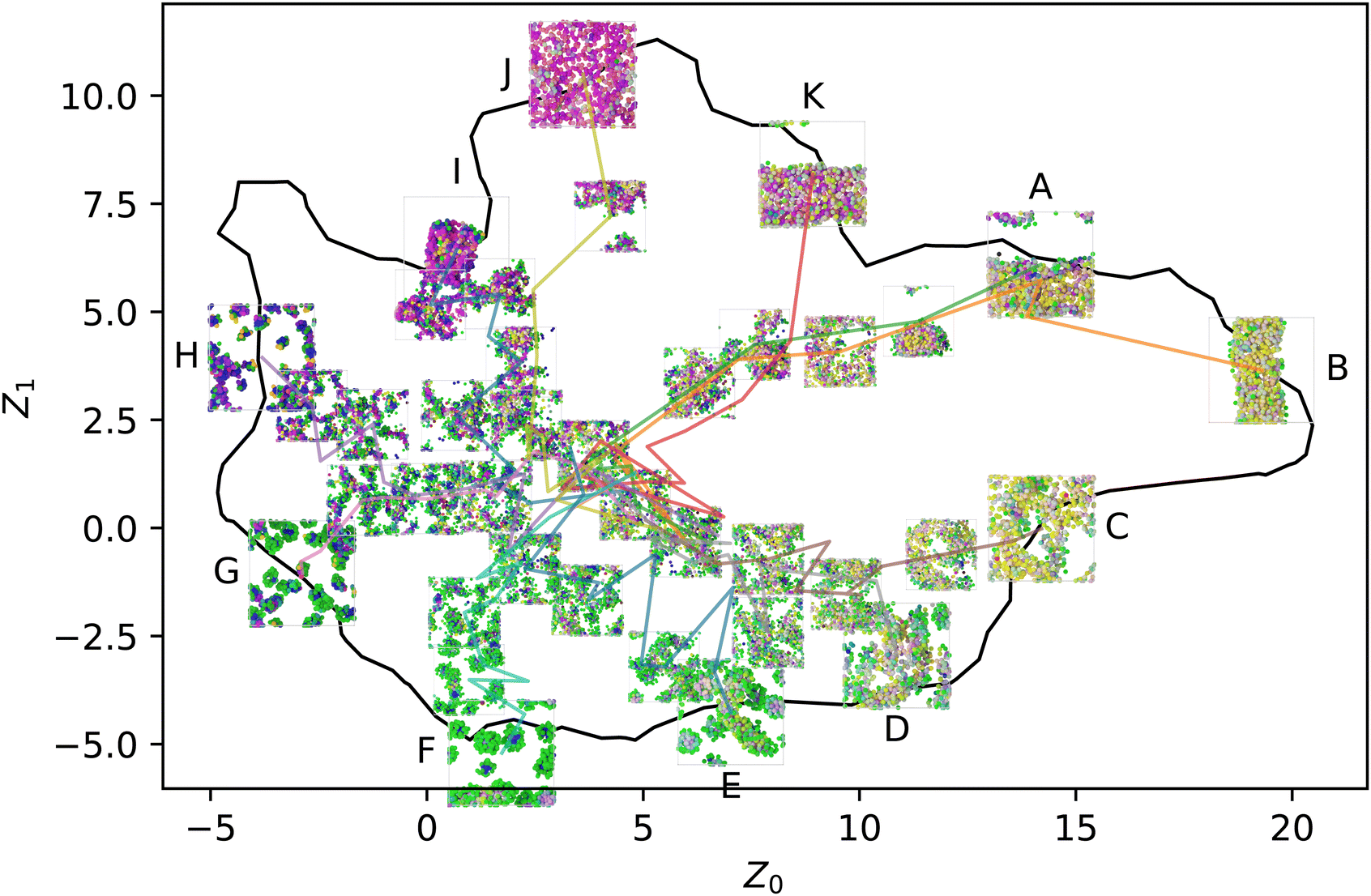Fig. 4 Selected p series from the periphery of the manifold: initially liquid (A) and (B), structured liquid (C)–(E), spherical micelles (F) and (G), wormlike micelles (H), membranes (I) and (J), and vesicles (K). The color scheme is the same as Fig. 2 and ref. 20, with each bead being colored in RGB space according to its position in the local environment manifold.

On the other hand, the appearance of common pathways on which several different peripheral sequences collapse is not expected. This can be seen especially with the structures labeled K, A, and B, where 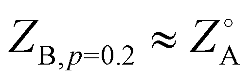and Z_B,p=0.4 ≈ Z_A,p=0.2 ≈ Z_K,p=0.1. This indicates that introducing finite p to some sequences drives them towards the template state of others, though no obvious trend appears to the authors in evaluating the sequences by eye: K, AABAABBAAABBBAAABAAB; A, ABABAABBBAABAAAABAAB; B, ABAABAABBAABABABAAAB.

We will hereafter refer to the collection of Z embeddings for a single sequence at different p as a series. Note that the various series shown in Fig. 4 are independently equilibrated at each p, so there is no hysteresis, and the use of lines to connect the different snapshots in the figure is purely for clarity in associating different points with the same series. Furthermore, the figure shows only one of the five replicas simulated for each (sequence, p) pair, so the plot appears quite noisy; averaging over the replicas helps resolve this noise to reveal more consistent trends.

Another view of the same series is shown in Fig. 5. This time, the series is laid out on a grid, with rows representing a common sequence and columns representing a common p. This view clearly shows the gradual convergence of the different sequences to a common, randomized morphology as p → 1. Each panel in Fig. 5 corresponds to a point along the lines in Fig. 4, where tracing the lines from exterior to interior is equivalent to following the series from left to right along a single row.

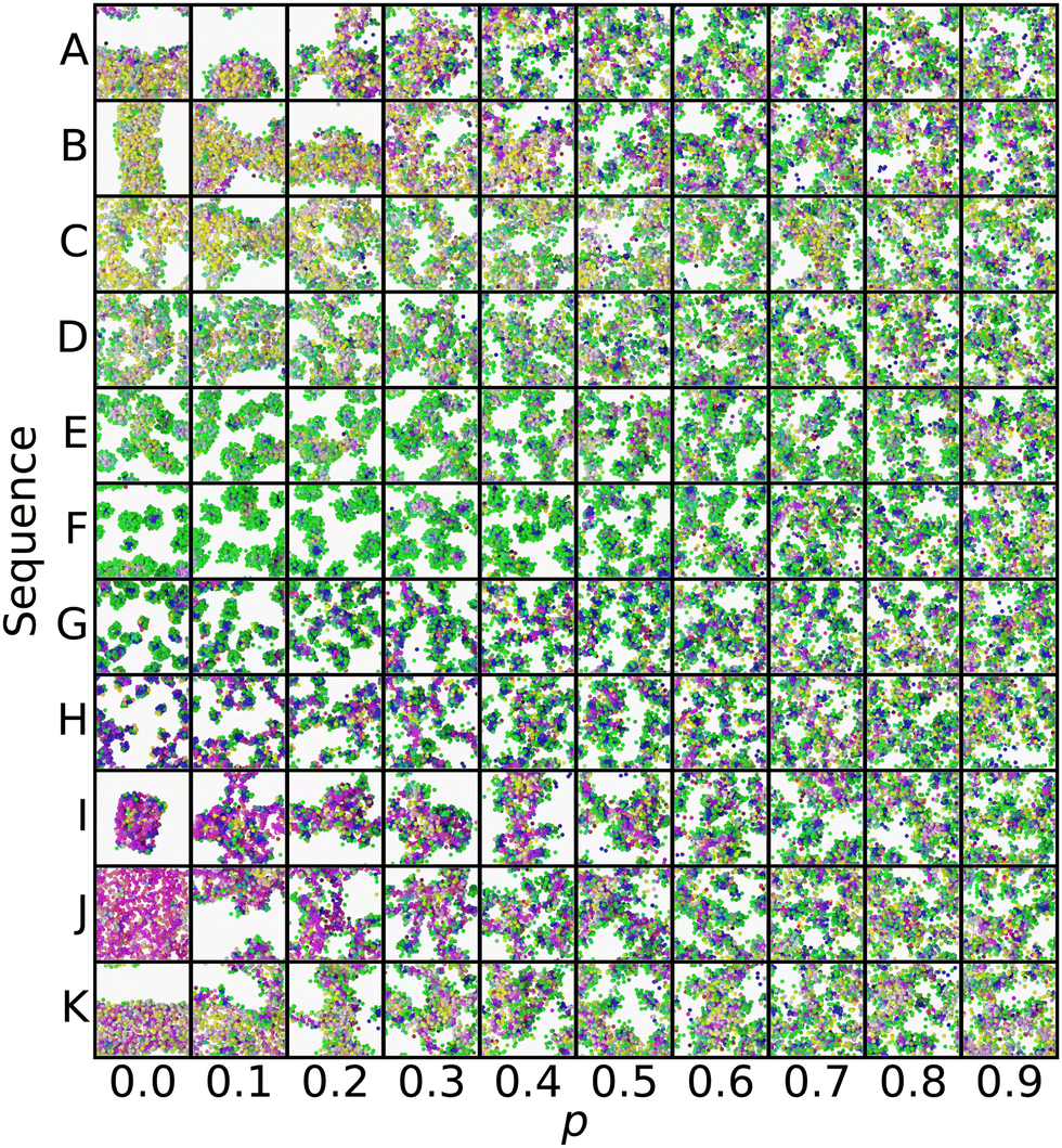Fig. 5 Grid view of the same series selected in Fig. 4, including simulation snapshots at more p values. The color scheme is the same as Fig. 2 and 4, and ref. 20, with each bead being colored in RGB space according to its position in the local environment manifold.

In evaluating Fig. 4 and 5, we found that spherical micelles (F, AAAAAAABABAABABBBABB) could tolerate more sequence variability than any other structure, remaining micelle-like for p < 0.5. This property extended to adjacent structures E (AABAAAAAAABBAABABBBB) and G (AABBABABBAAAAAAABBAB), which were also able to sustain their approximate structure for p < 0.4. On the other hand, membranes (J, AABBBAABABAAABAAAABB) broke down as soon as p > 0. We analyzed the magnitude of deviation from each sequences template Z° in Fig. 6. While most sequences could tolerate p = 0.1 variability without substantial morphology change, there were some notable outliers, including the liquid, vesicle, and membrane regions of the manifold. These outliers show the structural instability of these three aggregate morphologies when undergoing sequence variation and show that even small changes in sequence can lead to large structural changes.

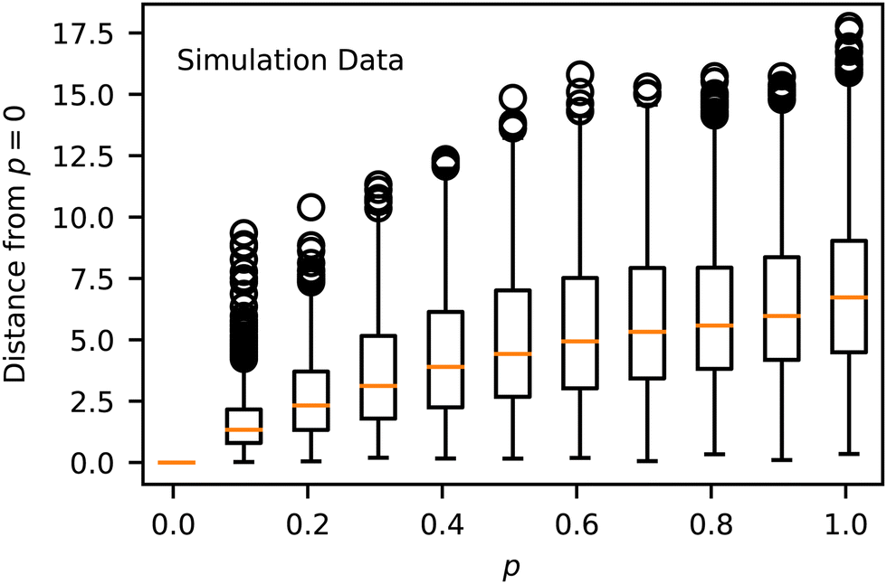Fig. 6 Euclidean distance from Z° as a function of p.

We hypothesize that the relative structural stability of spherical micelles under greater sequence variation is due to the longer block sequences present in the spherical micelle sequence that remain comparatively unaffected by minor sequence variation. Sequences defined by patterns of long blocks still contain comparatively long blocks when variability is introduced, and thus, the overall pattern remains intact. For sequences defined by patterns of short blocks, small changes in sequence disrupt the pattern more, and the short blocks in the simulation look different both from the template sequence and from each other.

This can be verified by evaluating the sequences most and least prone to deviation in Z. For the p = 0.1 case, the template sequences that are most sensitive to sequence variation are AAABAABAABAAAABABBBB, AAABAABAABAAAABABBBB, and AAABAABAABAAAABABBBB, and the least sensitive are ABBAAABAAABAAAABBBBA, ABAABABABBABAABAAAAB, and ABBAABABAABAABAABAAB. A value of p = 0.1 corresponds to an average of one flipped bead per chain (two selected for flipping, probability of 1/2 to flip). This means that the difference between most and least sensitive chains involves disruptions to the patterns of only a single bead on average. Therefore, it is not surprising that it is difficult or impossible to identify features of these sequences that lead to this result by eye. Instead, like in our prior work,²¹ we must rely on data-driven models to identify such patterns reliably.

3.2 Predicting morphology response

Bayesian hyperparameter tuning resulted in the following: learning rate of 2.75 × 10⁻³, 1185 training epochs, 4 hidden layers, number of neurons (79, 67, 56, 45), and ReLU activations. When the aggregates were simulated, they were replicated five times from the same starting conditions, which leads to variation between identical model inputs. Due to UMAP approximately maintaining topological structure, there are smooth structural transitions between nearby points on our manifold, which was expected. Previously, we found this intrinsic variance to be characterized by a Root Mean Square Deviation of approximately 0.67 (arbitrary units). The trained model gave RMSE = 1.044 on the validation set (used for selection of the hyperparameters) and RMSE = 0.909 on the test set (held out entirely from training optimization), which is only about 50% higher than the intrinsic randomness in the self-assembly process.

The resulting model allows us to predict the evolution of a series (i.e., fixed sequence, varying p) through the manifold, as shown in Fig. 7. There, we view the trajectories of archetypal (i.e., Z° on the manifold periphery) aggregate structures through the manifold as a function of p. As in Fig. 4, we see the model predicting some preferred paths, namely the S-shaped curve from the liquid region to the area of most randomness. It is interesting that the sequences take a non-linear path, as this indicates that there is some preferential architecture in this area; an explanation for this preference requires further investigation.

Fig. 7 Predicted series for archetypal structures colored by p, trained on 8547 self-assembled structures. Non-linear paths are observed through the manifold, along with some seemingly preferred regions.

We analyzed the model error as a function of p and Z, shown in Fig. 8 and 9, respectively. The error has a slight peak around p = 0.3 but otherwise remains relatively flat for all p > 0, demonstrating that the model accurately predicts the influence of p. Note that the training error for all p is just above the RMSD of approximately 1.0 identified above, indicating that the NN model is learning the trends in the training data almost perfectly. The validation and test errors are slightly higher, but the standard deviations are so large that this effect is relatively small. We also analyzed the error as a function of Z to identify possible bias towards certain morphologies. There is no discernible pattern in Fig. 9, indicating no difference in the error rate across different sequences or structures. It is noteworthy that the model seems to perform equally well in previously identified outlier regions (e.g., from Fig. 6).

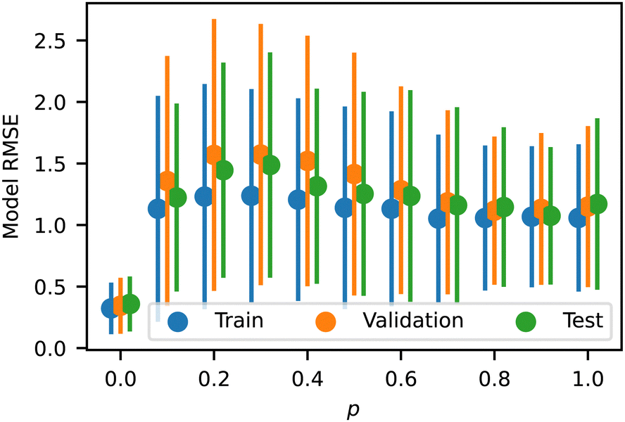Fig. 8 Model RMSE as a function of p for the training, testing, and validation datasets. Error bars indicate standard deviation.

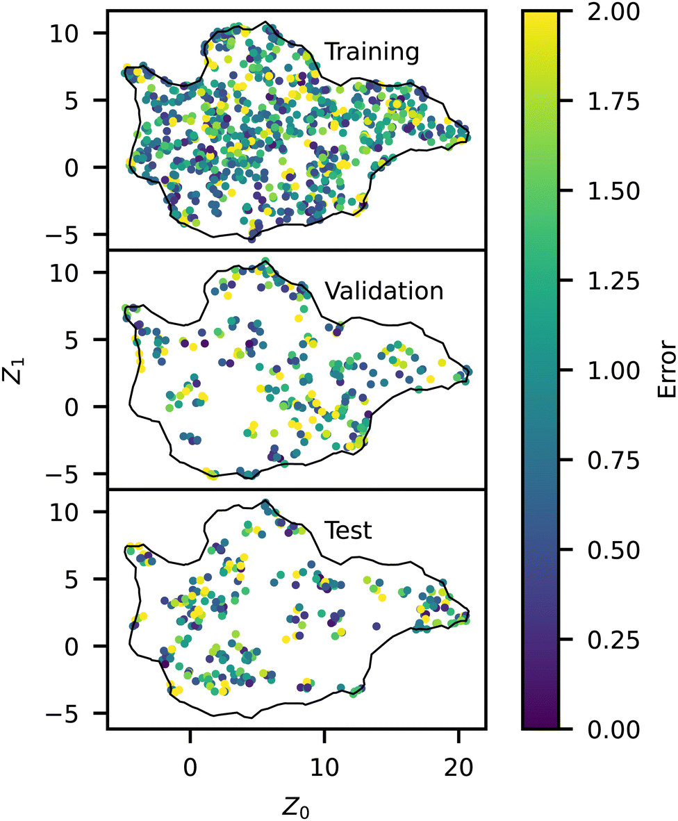Fig. 9 Spatial representation of model RMSE across the manifold for the training, testing, and validation datasets, colored by the error.

3.3 Model sensitivity

In addition to the predictive capabilities of our trained surrogate model, it also has the benefit of smoothing the stochastic response in order to more clearly show general trends in the data. We analyzed the magnitude of the gradient (which we refer to as sensitivity) throughout the manifold using the trained NN model and plotted this quantity for different p in Fig. 10. The sensitivity is highest in the liquid, membrane, and string morphologies for low p, especially around p = 0.2. As p increases, the magnitudes decrease for these regions since the structures are already close to completely random after this point. As p → 1, it is statistically more difficult to drive these structures away from Z° since they are already mostly random, so the embedded representations of these structures also move less. The previous qualitative analysis of the simulation data also arrived at this conclusion, as the outliers in Fig. 6 occurred mainly in the liquid, membrane, and vesicle regions. On the other hand, we see that the micelle region (bottom left) of the manifold is relatively insensitive to p and only experiences an appreciable gradient at p = 0.8. This is partly due to being closer to Z^R to begin with but also appears to be related to the sequence itself, with smaller p being less disruptive to the long blocks.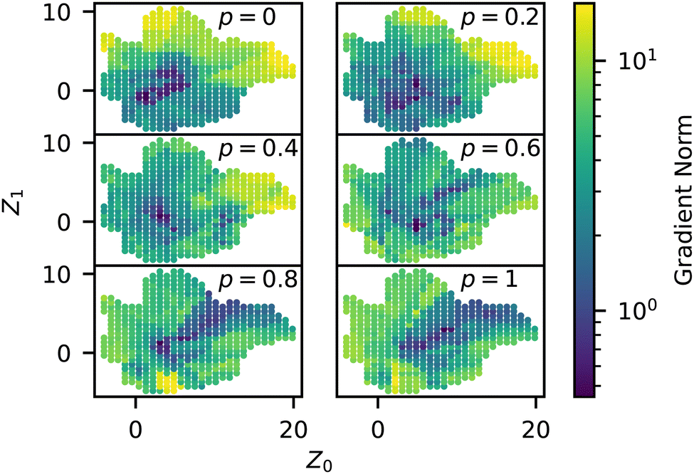

Fig. 10 Norm of the trained model gradients across the manifold for different values of p, colored by the norm (i.e., eqn (2)).

4 Conclusions

In this work, we demonstrate the application of machine learning to predict the morphological response of self-assembled aggregates to stochastic sequence variation in a model sequence-controlled copolymer. The incorporation of stochastic variation in monomer sequences while keeping their length fixed allows us to investigate sequence sensitivity and enables our design scheme to mimic variations present in real-world polymer systems. The objective of this work, therefore, was to quantitatively predict how a given template sequence undergoing a given level of mutation p leads to changes in self-assembled aggregate morphology.

We generated a dataset of 14 795 MD simulation trajectories of 259 monomer sequences with 11 variations of p ranging from 0 to 1 in intervals of 0.1, representing nearly 2000 GPU hours of compute time on NVIDIA A100 GPUs. An unsupervised representation learning technique developed in our recent work²⁰ was applied to learn relevant order parameters. Supervised learning was then used to predict the effect of independent random sequence variation at rate p within each chain via a shallow NN. This model was then analyzed to identify patterns across the entire morphology space and to quantitatively describe the simulation results.

From the MD simulations, we found that liquids, membranes, and vesicles were more sensitive to sequence randomness than other aggregate structures, as indicated by the large number of statistical outliers present in these regions when analyzing the morphology deviation as a function of p. This observation is consistent with the explanation that sequences defined by small blocks have relatively high sensitivity to single monomer edits compared to sequences defined by large blocks.

We also observed that the series tended to progress through the manifold between Z° and Z^R via a relatively jagged and stochastic path, requiring averaging over many replicas in order to obtain reliable trends. We have previously shown that the Z order parameters are smooth within the dynamics of a single simulation,²⁰ so when it occurs, this shows that small perturbations to the sequence can lead to relatively large changes in morphology.

Despite the stochastic nature of the self-assembly process, our supervised NN performed well, resulting in a validation RMSE of 1.04, slightly lower than the observed RMSD of 1.07 from simulation replicas; this indicates that performance is on par with the intrinsic variance from self-assembly. The model showed no bias toward either particular p (aside from p = 0 performing well) or Z, indicating that it is equally valid across the entire manifold. The model also revealed some interesting contours in the trajectories of sequence embeddings throughout the manifold. Preferred pathways were visible, indicating collapse onto locally common aggregate structures during randomization. The underlying reason for these preferred intermediate morphologies will require further study. Spatial analysis of model gradients showed the largest structural shifts around the liquid, membrane, and vesicle areas of the manifold, quantitatively describing the previously observed sensitivity to sequence variation in these areas.

We have shown that stochasticity in chemical sequences can profoundly affect self-assembly and that this affects different sequences to very different degrees depending on their characteristics. This is an important step towards understanding the potential and limitations of sequence-controlled polymers with imperfect chemical sequences, as typically synthesized in the laboratory. We have demonstrated that our previously developed framework can be applied to study stochastic sequences and, together with the supervised learning approach deployed here, may be useful for probing the robustness of a particular morphology against sequence variations. We believe this is an important design consideration as computational tools converge with experimental applications. In future work, we will consider more complex chain structures, including varying lengths and sequences simultaneously, further to align our models with attainable, real-world chemical systems.

Author contributions

Kaleigh Curtis: software, data curation, investigation, writing – original draft, writing – review and editing, visualization. Antonia Statt: software, conceptualization, writing – review and editing. Wesley Reinhart: conceptualization, software, data curation, writing – original draft, writing – review and editing, visualization, supervision.

Data availability

All data and code for this article are available on Zenodo at https://doi.org/10.5281/zenodo.11507385.

Conflicts of interest

There are no conflicts to declare.

Acknowledgements

This material is based upon work supported by the National Science Foundation under Grant No. DMR-2401663 and DMR-2401664. We acknowledge the Pennsylvania State University Institute for Computational and Data Sciences (ICDS) for computational resources and financial support and the Department of Materials Science and Engineering for financial support.

Notes and references

1. P. Weiss, J. Polym. Sci., Polym. Lett. Ed., 1978, 16, 151–152.
2. C. Li, Q. Li, Y. V. Kaneti, D. Hou, Y. Yamauchi and Y. Mai, Chem. Soc. Rev., 2020, 49, 4681–4736.
3. C. K. Wong, X. Qiang, A. H. Müller and A. H. Gröschel, Prog. Polym. Sci., 2020, 102, 101211.
4. A. Rösler, G. W. M. Vandermeulen and H.-A. Klok, Adv. Drug Delivery Rev., 2012, 64, 270–279.
5. H. Feng, X. Lu, W. Wang, N.-G. Kang and J. W. Mays, Polymers, 2017, 9, 494.
6. C. Park, J. Yoon and E. L. Thomas, Polymer, 2003, 44, 6725–6760.
7. Y. Mai and A. Eisenberg, Chem. Soc. Rev., 2012, 41, 5969–5985.
8. D. Dolgov, T. Grigorev, A. Kulebyakina, E. Razuvaeva, R. Gumerov, S. Chvalun and I. Potemkin, Polym. Sci., Ser. A, 2018, 60, 902–910.
9. S. Li, C. Yu and Y. Zhou, Sci. China: Chem., 2019, 62, 226–237.
10. S. Cui, L. Yu and J. Ding, Macromolecules, 2019, 52, 3697–3715.
11. D. Liu, H. Sun, Y. Xiao, S. Chen, E. J. Cornel, Y. Zhu and J. Du, J. Controlled Release, 2020, 326, 365–386.
12. A. R. Khokhlov and P. G. Khalatur, Phys. A, 1998, 249, 253–261.
13. M. A. Webb, N. E. Jackson, P. S. Gil and J. J. de Pablo, Sci. Adv., 2020, 6, eabc6216.
14. A. A. Bale, S. M. Gautham and T. K. Patra, J. Polym. Sci., 2022, 60, 2100–2113.
15. J. Shi, M. J. Quevillon, P. H. Amorim Valenca and J. K. Whitmer, ACS Appl. Mater. Interfaces, 2022, 14, 37161–37169.
16. P. S. Ramesh and T. K. Patra, Soft Matter, 2023, 19, 282–294.
17. V. Meenakshisundaram, J.-H. Hung, T. K. Patra and D. S. Simmons, Macromolecules, 2017, 50, 1155–1166.
18. T. K. Patra, T. D. Loeffler and S. K. Sankaranarayanan, Nanoscale, 2020, 12, 23653–23662.
19. T. Zhou, Z. Wu, H. K. Chilukoti and F. Muller-Plathe, J. Chem. Theory Comput., 2021, 17, 3772–3782.
20. A. Statt, D. C. Kleeblatt and W. F. Reinhart, Soft Matter, 2021, 17, 7697–7707.
21. D. Bhattacharya, D. C. Kleeblatt, A. Statt and W. F. Reinhart, Soft Matter, 2022, 18, 5037–5051.
22. G. Gody, P. B. Zetterlund, S. Perrier and S. Harrisson, Nat. Commun., 2016, 7, 10514.
23. J. D. Neve, J. J. Haven, L. Maes and T. Junkers, Polym. Chem., 2018, 9, 4692–4705.
24. H. K. Murnen, A. R. Khokhlov, P. G. Khalatur, R. A. Segalman and R. N. Zuckermann, Macromolecules, 2012, 45, 5229–5236.
25. H. Mutlu and J.-F. Lutz, Angew. Chem., Int. Ed., 2014, 53, 13010–13019.
26. M. Porel and C. A. Alabi, J. Am. Chem. Soc., 2014, 136, 13162–13165.
27. G. L. Sternhagen, S. Gupta, Y. Zhang, V. John, G. J. Schneider and D. Zhang, J. Am. Chem. Soc., 2018, 140, 4100–4109.
28. A. J. DeStefano, R. A. Segalman and E. C. Davidson, JACS Au, 2021, 1, 1556–1571.
29. A. J. DeStefano, S. D. Mengel, M. W. Bates, S. Jiao, M. S. Shell, S. Han and R. A. Segalman, Macromolecules, 2024, 57, 1469–1477.
30. T.-S. Lin, C. W. Coley, H. Mochigase, H. K. Beech, W. Wang, Z. Wang, E. Woods, S. L. Craig, J. A. Johnson, J. A. Kalow, K. F. Jensen and B. D. Olsen, ACS Cent. Sci., 2019, 5, 1523–1531.
31. D. Weininger, J. Chem. Inf. Comput. Sci., 1988, 28, 31–36.
32. S.-M. Hur, C. J. García-Cervera, E. J. Kramer and G. H. Fredrickson, Macromolecules, 2009, 42, 5861–5872.
33. S. M. Blinder, Am. J. Phys., 1965, 33, 431–443.
34. M. W. Matsen, Eur. Phys. J. E: Soft Matter Biol. Phys., 2009, 30, 361.
35. M. W. Matsen and F. S. Bates, Macromolecules, 1996, 29, 7641–7644.
36. W. S. Loo, M. D. Galluzzo, X. Li, J. A. Maslyn, H. J. Oh, K. I. Mongcopa, C. Zhu, A. A. Wang, X. Wang, B. A. Garetz and N. P. Balsara, J. Phys. Chem. B, 2018, 122, 8065–8074.
37. J. Jones, Proc. R. Soc. London, Ser. A, 1924, 106, 441–462.
38. J. D. Weeks, D. Chandler and H. C. Andersen, J. Chem. Phys., 1971, 54, 5237–5247.
39. K. Kremer and G. S. Grest, J. Chem. Phys., 1990, 92, 5057–5086.
40. J. A. Anderson, J. Glaser and S. C. Glotzer, Comput. Mater. Sci., 2020, 173, 109363.
41. W. F. Reinhart, Comput. Mater. Sci., 2021, 196, 110511.
42. L. McInnes, J. Healy, N. Saul and L. Großberger, J. Open Source Software, 2018, 3, 861.
43. W. Reinhart and D. Bhattacharya, sdmm-regression, 2022, https://github.com/wfreinhart/sdmm-regression.
44. K. Curtis, A. Statt and W. Reinhart, Data for “Predicting self-assembly of sequence-controlled copolymers with stochastic sequence variation”, 2024 DOI:10.5281/zenodo.11507385.
45. F. Pedregosa, G. Varoquaux, A. Gramfort, V. Michel, B. Thirion, O. Grisel, M. Blondel, P. Prettenhofer, R. Weiss, V. Dubourg, J. Vanderplas, A. Passos, D. Cournapeau, M. Brucher, M. Perrot and E. Duchesnay, J. Mach. Learn. Res., 2011, 12, 2825–2830.
46. A. Paszke, S. Gross, F. Massa, A. Lerer, J. Bradbury, G. Chanan, T. Killeen, Z. Lin, N. Gimelshein and L. Antiga, et al., Adv. Neural Inf. Process. Systems, 2019, 32, 8026–8037.
47. E. Bakshy, L. Dworkin, B. Karrer, K. Kashin, B. Letham, A. Murthy and S. Singh, Conference on neural information processing systems, 2018, pp. 1–8.

---