An integrated experimental-computational investigation of the mechanical behavior of random nanofiber networks

Abstract

An integrated experimental-computational methodology was developed to study the mechanical behavior of random polymer nanofiber networks with controlled network structural parameters. Random nanofiber networks, comprised of continuous polyethylene oxide (PEO) nanofibers with ∼250 nm diameter and controlled mean fiber segment length, were designed with a computer algorithm and printed via near-field electrospinning. The structure of the same networks served as input to a computational model to obtain predictions of the macroscopic mechanical response. This methodology provides consistency in fabricating, testing and simulating nominally identical random fiber networks. Specimens with 500 to 5000 nanofibers were subjected to uniaxial tension and compared to modeling predictions for the network mechanical behavior. The predictions by the computational model, with inputs from the experimental network structure, the measured single PEO nanofiber properties, and the fiber crimp parameter, agreed with the experimental results both quantitatively and with respect to the dependence of the measured quantities on the network parameters. The network stiffness and strength followed a power-law scaling with the network density, with exponents 2.78 ± 0.15 and 1.59 ± 0.04, respectively, while the network stretch at failure gradually decreased with increasing network fiber density. Finally, the experimentally determined network toughness demonstrated a rather weak power-law dependence on the network fiber density (exponent of 1.18 ± 0.12).

---

1. Introduction

Nanofiber networks provide versatility in tailoring their mechanical properties by controlling their structural parameters. This makes them useful in a variety of applications,^1–5 such as air filtration and water purification,⁶ and tissue scaffolds for wound healing.⁷ Most networks can be classified as either thermal or athermal. In thermal networks, the temperature significantly influences the network mechanical behavior, while in athermal networks fiber interactions such as crosslinking dominate. Athermal networks can be described in terms of the network structural parameters, such as the nanofiber diameter, d, the fiber orientation, the fiber density, ρ, and the crosslink density, ρ_b. The effective network properties are further controlled by the mechanical properties of individual nanofibers and their interactions at contacts and crosslinks. In the past, a significant body of research has been focused on quantifying the mechanical properties (elastic modulus, tensile strength, and ductility) of individual nanofibers through various experimental modalities.^8–12 More recently, a systematic study using precision Microelectromechanical System (MEMS) tools and contact mechanics analysis quantified the normal and shear detachment of pairs of electrospun nanofibers under quasi-static¹³ and dynamic loading conditions.¹⁴ Yet, experimental studies of the mechanical response of nanofiber networks, are still lacking albeit all nanofiber applications involve networks of nanofibers.

On the other hand, several computational studies have explored the effect of network parameters on the effective and local mechanical behavior.^15–20 These studies led to a general understanding of structure–property relationships.²¹ The small strain stiffness, E₀, and the fiber density (defined as the total length of fibers per unit volume in 3D, or area in 2D) are related through a power law, E₀ ∼ ρ^x, where the exponent depends on the type of network and assumes larger values in 2D than in 3D networks.^22–25 If the network is sufficiently dense and densely cross-linked to deform approximately affinely, E₀ is proportional to ρ, i.e. x = 1.²⁶ The ultimate tensile strength (UTS) of the network is proportional to the density, UTS ∼ ρ, as established by modeling^19,27,28 and confirmed experimentally for certain networks.^29,30 Beyond the peak stress, networks may fail either in a brittle manner by propagation of a major crack, or may exhibit gradual failure due to accumulation of diffuse damage that does not coalesce to form a major crack. This second mechanism leads to a large toughness. In these cases, the toughness has been computed to be proportional to UTS.³¹ This proportionality does not apply to the more brittle regime where failure is caused by the unstable propagation of a dominant crack and diffuse damage contributes less to the overall energy dissipation. In general, if fibers are weaker than the crosslinks and fail first, the network rupture is brittle and toughness is low, while if crosslinks fail before the fibers, the network rupture is more ductile, and the toughness is large.

If the fiber and the crosslink strength are described by distributions and vary across a given network, the network strength is lower than in the case where all fibers or crosslinks have the same strength and are equal in value to the mean of the respective distribution.^22,32 This result is relevant to post-fabrication treatments, such as crosslinking and annealing of a network,^33–36 that have been effective in changing the network structural parameters and hence its mechanical response.

Contrary to the aforementioned wealth of information derived from computational studies, a quantitative experimental evaluation of structure–property relationships in nanofiber networks is lacking due to challenges in determining the network structure which, in turn, prohibits an accurate evaluation of the network parameters. While recent advances in network graph theory³⁷ may provide a means to quantify the network structural parameters, collection and processing of statistical (imaging) data from large network areas remains a challenge especially for polymeric nanofibers that are susceptible to electron microscopy imaging damage. In order to facilitate a direct comparison between modelling predictions and experimental data, it is important to control nanofiber positioning during network fabrication. Conventional electrospinning has been widely used to generate stochastic networks, but this method does not provide control of the network structure due to the associated polymer solution jet instabilities.^38,39 The need for precise nanofiber positioning can be addressed by near-field electrospinning^40–43 that operates at reduced nozzle to collector distances (<1 mm) and applied voltages (<1000 V) compared to conventional electrospinning. These conditions prevent the onset of spinning and bending instabilities of the jet and allow for spatially accurate nanofiber positioning to construct networks with controlled structural parameters.

In this research, an integrated experimental and computational methodology was developed to investigate the mechanical behavior of polymer nanofiber networks with emphasis on the synthesis and testing of networks with controlled structural parameters. This experimental methodology enables developing computational models that reproduce the exact structure of a physical network, which, in turn, could be used to infer network properties that are beyond what could be determined experimentally. A near-field electrospinning system was built to print networks of polymer nanofibers and determine, both experimentally and computationally, the effect of network density on the network stiffness, strength, ductility and toughness.

2. Materials and methods

2.1. Experimental methodology

Poly(ethylene oxide) (PEO) nanofibers with an average molecular weight of M_v = 400 000 g mol⁻¹ (Sigma-Aldrich) were electrospun using a 10 wt% PEO solution in de-ionized (DI) water that was mixed at room temperature for 12 h. A home-built near-field electrospinning apparatus was used to deposit the nanofiber networks onto a gold-coated silicon wafer in Fig. 1(a). The applied voltage, the distance between the tip of the polymer solution droplet emerging from a fine needle and the Si-wafer collector, the polymer solution concentration, and the collector speed influence the nanofiber diameter^43,44 and morphology.

Fig. 1 Schematics of (a) near-field electrospinning apparatus, and (b) mechanical testing device used for uniaxial tension testing of electrospun nanofiber networks. The inset shows the design of a network consisting of 500 fibers.

A systematic parametric study (ESI†) was conducted to determine the near-field electrospinning parameters that result in continuous and straight PEO nanofibers with ∼250 nm diameter and limited adhesion to the Si-wafer collector for easy removal and mechanical testing of the network. A collector speed of 31 mm s⁻¹ was selected to lay straight PEO nanofibers, Fig. S1 (ESI†). An optimal set of values for the rest of the near-field electrospinning parameters included an applied voltage of 800 V, a needle-to-collector distance of 0.5 mm, and a PEO solution concentration of 10 wt%. These conditions also allowed for sufficient solvent evaporation during electrospinning, which reduced the adhesion of PEO fibers to the collector and facilitated the successful lift-off of the printed nanofiber networks from the collector.

The network structure was generated in Python using an algorithm that placed straight fibers with their ends at the boundaries of a 16 mm × 8 mm rectangular frame. The end points of each fiber were selected at random on this rectangular frame. To avoid bridging fibers that would directly connect the loading grips and dominate the mechanical behavior of the entire network, the fiber angle was allowed to vary in the range of 20°–80° with respect to the uniaxial loading direction. The fiber end coordinates were provided to a home-built apparatus that controlled the movement of the near-field electrospinning print head. This approach allowed printing many copies of the same networks with 500, 1000, 3000 and 5000 nanofibers, e.g. inset in Fig. 1(b). The network densities corresponding to these fiber numbers were 28 mm⁻¹, 56 mm⁻¹, 169 mm⁻¹ and 281 mm⁻¹, respectively. This network synthesis method also allows for repetition of mechanical experiments with nominally the same networks (i.e. networks with different microstructure but the same structural parameters).

The printed networks were lifted off from the collector surface with the aid of a rectangular polydimethylsiloxane (PDMS) window of 8 mm × 4 mm (outside window frame dimensions 20 mm × 10 mm) fabricated by using a Sylgard 184 silicone elastomer. The nanofibers adhered to the PDMS window frame to form freestanding network specimens with dimensions of 8 mm × 4 mm. This network specimen size was determined by the largest possible field of view provided by the available, aberration corrected, optical microscope objective that was used during mechanical testing. The network specimen size was also evaluated for finite-size effects. A very large network size compared to the mean fiber segment length is required to reduce finite specimen size effects. This condition was evaluated for our networks by using existing literature on random fiber network size effects.^45,46 Using the results in ref. 45 it was determined that the PEO nanofiber networks tested in this study were sufficiently large compared to the mean fiber segment length, and therefore finite-size effects are expected to be rather small.

After lift-off the printed networks were annealed in an oven for 10 min at 60 °C. This temperature was chosen to promote bonding (cross-linking) between nanofibers because it is slightly below the melting point of PEO (65 °C), and also assist with the evaporation of residual solvent (water). After mounting a PDMS window frame with the PEO nanofiber network onto the mechanical testing apparatus, Fig. 1(b), the PDMS frame edges that were parallel to the loading direction were cut and separated from the network by locally dissolving the PEO nanofibers with de-ionized (DI) water. During network stretching, the mechanical testing apparatus, Fig. 1(b), was designed to maintain the test specimen in the field of view of an upright optical microscope with a 2.5× objective lens, which was used to capture images of the fiber network during tensile testing. Additionally, a horizontal optical microscope equipped with a 1.4× objective lens was used to record the motion of the specimen grips during testing. A random speckle pattern, consisting of circular speckles with a diameter of 0.2 mm (Speckle Generator, Correlated Solutions, Inc.), was applied to the sides of the specimen grips. The rigid-body displacement of the grips was determined via Digital Image Correlation (DIC) (VIC-2D, Correlated Solutions, Inc.), from which the macroscopic stretch ratio of a fiber network was calculated. The applied force was measured with a high resolution loadcell (Futek LPM 200) with 100 mN force capacity and 0.01 mN resolution.

The mechanical properties of individual PEO fibers, serving as input to the computational model, were obtained through uniaxial tension tests using a MEMS-based method.^9,10 A recent modification of this method using real-time edge detection instead of DIC, was implemented to measure the force and the stretch ratio of individual PEO nanofibers.^47,48 The diameter of the individual nanofibers was determined from images obtained via scanning electron microscopy (SEM), as described in ref. 11. Prior to mechanical testing, high-resolution images of the nanofiber networks were obtained using a scanning laser confocal microscope (Keyence VK-X1000) equipped with a 5× objective lens. Stitched images with a resolution of 3652 × 2080 pixels provided detailed visualization of the network structure. A Hitachi S-4800 high-resolution SEM was used to determine the nanofiber diameter distribution. The fibers were sputter-coated with Au–Pd to prevent charging and damage during SEM imaging that was conducted with a low accelerating voltage of 2 kV to minimize beam-induced damage and heating effects that would alter the fiber morphology. A ThermoFisher Axia ChemiSEM in low vacuum mode was used to measure the mean fiber segment length (l_c), which is the average distance between two adjacent crosslinks along a given fiber.

2.2. Computational modelling

Computational models were developed to replicate the exact structure of the printed networks. The network structure generated by the Python code and used for near-field electrospinning of the experimental networks served as the input in model generation. All fiber overlaps were initially treated as crosslinks. This is expected in the physical network specimens because of (a) thermal annealing that was applied after network deposition, and (b) the relatively low density of nanofibers resulting in considerably large distances between cross-link points (e.g. this averages 6030 nm for networks with 5000 fibers) compared to the average nanofiber diameter (250 nm). The fibers were discretized while ensuring that nodes were placed at all crosslinks. Each fiber was discretized into multiple two-node linear Timoshenko beam elements (B21 element in Abaqus), with the number of elements per fiber segment (defined by two successive crosslinks along a given fiber) being a function of the fiber segment length. The smallest element for discretization was determined based on the mesh convergence test shown in Fig. S2 of the ESI.† The test considered model cases with element lengths ranging from 50 μm to 0.5 μm for increasing mesh refinement level. In each case, segments shorter than the specified element length were eliminated by merging the respective crosslinks and nodes. Convergence of the effective stress (force/specimen width) vs. network stretch curves took place for a minimum element size of 1 μm. Therefore, this element length was used in all simulations. This procedure⁴⁹ provided a balance between modelling accuracy and computational cost.

Meshing resulted in 200 000 to 7 500 000 elements for networks ranging between ρ = 28 mm⁻¹ (500 fibers) to 281 mm⁻¹ (5000 fibers). All fibers in the model were considered to have the same diameter, which was determined as described in Section 2.1. Due to thermal annealing, the fiber crosslinks were considered of ‘weld’ type, i.e. the crosslinks allowed transmitting forces and moments between fibers and along each fiber. Electron microscopy observations confirmed fiber fusion at contacts after thermal annealing, as shown in Fig. 2(a). Moreover, some degree of fiber crimping was observed after lift-off. Fiber crimping could arise from pre-strain or fiber undulations⁵⁰ during network printing or from external factors such as thermal excitations.⁵¹ In this study, crimping was introduced during network lift-off. All PEO fibers were laid straight on the Si-wafer by controlling the collector speed during near-field electrospinning (Fig. 2(b)). However, the network had to be gradually lifted off (peeled) the Si-wafer, causing crimping due to relative fiber movement. Subsequent thermal annealing at 60 °C created permanent cross-links between fibers but did not change the crimping. The crimp parameter (ratio between the end-to-end length and the contour length of each fiber segment) was measured in the physical samples. In the model, all fibers were given a uniform crimp parameter value equal to the mean of the experimental crimp distribution.

Fig. 2 (a) SEM image showing fiber fusion at crosslinks after annealing. (b) Optical image at 20× magnification of as-printed straight PEO fibers. (c) and (d) Optical images at 5× magnification showing fiber rupture between two cross-link points.

The boundary conditions applied to the computational model represented the experimental setup: the model edges attached to the rigid grips were subjected to displacements in the loading direction, while preventing the displacement of these boundary nodes in the direction orthogonal to loading. The edges parallel to the loading direction were traction-free. Finally, in order to account for lateral contraction taking place after releasing the network from the lateral supports in the PDMS window frame, the undeformed network model shape was modified by the amount of hourglassing measured in the annealed specimens.

The fiber mechanical behavior was defined by stress-stretch curves (Fig. 3) obtained from tests on individual PEO nanofibers. These tests also provided elastic-plastic material data and the individual fiber strength, which were used to define fiber damage (maximum stress sustained by individual fibers) in the computational model, and thus model damage initiation and evolution in the network. Experimental observations confirmed that damage proceeded by fiber failure rather than by crosslink rupture, as shown in Fig. 2(c and d).

Fig. 3 Tensile behaviour of individual PEO nanofibers and derived properties (table). Inset: SEM image of a PEO nanofiber section. The scale bar corresponds to 500 nm.

The fully non-linear (both material nonlinearity and geometric nonlinearities, i.e. large rotations and deformations, were accounted for) and quasistatic simulations were performed with Abaqus Explicit (version 2022). Abaqus Explicit utilizes a central difference-based forward time marching algorithm and for nonlinear formulation it uses explicit dynamic integration methods. To ensure quasistatic conditions, inertia forces were minimized by artificially keeping the material density low and by introducing alpha damping with values in the range 0.01–0.1. Artificial mass scaling of short elements was used to improve the computational efficiency (for high density networks) while ensuring inertia forces are negligible. A variable mass scaling factor in the range of 10⁻⁶–10⁻⁸ was used, as short element lengths vary among different networks. The damping and mass scaling parameters were chosen to ensure that the kinetic energy remained a small fraction (<5%) of the total energy.⁴⁹ Enforcing this condition is relatively easy up to the peak force but becomes gradually more challenging in the post peak regime due to rapid damage accumulation.

3. Results and discussion

3.1. Individual PEO nanofiber properties

Fig. 3 shows the stress vs. stretch curves for three PEO nanofibers. The three experiments yielded an average Young's modulus of 1.96 ± 0.08 GPa and a mean stretch at failure of 1.06 ± 0.01. The high stiffness and low ultimate tensile strain of PEO fibers are attributed to partial crystallization occurring during thermal annealing at 60 °C, which increased their mechanical stiffness while reducing their ductility.⁵² The fiber diameter (table inset in Fig. 3) was measured at 20 different locations along each tested fiber, showing consistency with small fluctuations.

3.2. Characterization of network parameters

Examples of networks with four different nanofiber densities (corresponding to 500, 1000, 3000, and 5000 fibers in a 16 mm × 8 mm deposition area) are shown in Fig. 4(a–d). The corresponding network properties are provided in Table 1. The distribution of fiber diameters sampled from a network with all four densities is given in Fig. 4(e), with the average diameter being 243 ± 28 nm. The fiber diameter depends on the electrospinning parameters, i.e. applied voltage, needle-to-collector distance, and polymer solution density, and not on the number of fibers in a network, as shown in Fig. S3 of the ESI.† Based on our prior research,^11,12 the mechanical properties of electrospun nanofibers are expected to be quite uniform in this tight range of diameters. The mean segment length, l_c, was measured directly from the printed networks as the mean of the distribution of end-to-end segment lengths, with a segment being defined by two consecutive crosslinks along a fiber. A total of two hundred fiber segments from nine locations in each printed network were measured from SEM images. The experimental measurements and the model predictions using the print input are shown in Fig. 4(f) and are compared to l_c calculated from the 2D version of the Kallmes–Corte model:⁵³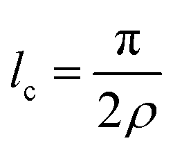which assumes a random distribution of fiber orientations. A good agreement was observed between the experimental l_cvs. ρ curve and the Kallmes–Corte model predictions, demonstrating that the printed networks approximated random fiber networks in terms of their structural parameters. The small (but systematic) difference between the experimental and the Kallmes–Corte theoretical values could be attributed to restrictions imposed on the orientation of the printed fibers to avoid bridging between the test grips, as described in Section 2.1.

Fig. 4 Printed PEO nanofiber networks with (a) 500 (ρ = 28 mm⁻¹), (b) 1000 (ρ = 56 mm⁻¹), (c) 3000 (ρ = 169 mm⁻¹) and (d) 5000 (ρ = 281 mm⁻¹) fibers. Scale bars are 1 mm. (e) Nanofiber diameter distribution compiled with data pooled from networks with all four densities. (f) Mean fiber segment length as a function of inverse network density. (g) Fiber crimp measured as the ratio of the actual contour length of each fiber segment (red line) to the fiber end-to-end length (orange line). (h) Experimental vs. simulation-derived force vs. stretch ratio curves of a network (ρ = 28 mm⁻¹) with and without fiber crimp.

Table 1 Network fiber density and crimp parameters

Number of fibers	Fiber density [mm^−1]	Fiber crimp
500	28	1.13 ± 0.08
1000	56	1.13 ± 0.05
3000	169	1.10 ± 0.04
5000	281	1.08 ± 0.03

---

A smaller albeit systematic difference was registered between the experimental and computational results. This difference is attributed to the fiber crimp which in the computational model was accounted only as the average value and not the distribution. Fiber crimping can significantly affect the mechanical behavior of nanofiber networks.^54,55 The crimp parameter, c, serves as a measure of the fiber waviness, and is defined as the ratio of the actual contour length of each fiber segment to the end-to-end fiber length, Fig. 4(g). A value of c = 1 corresponds to a completely straight fiber, while values much greater than 1 indicate a high degree of waviness. The crimp parameter was calculated using ImageJ software and images obtained via scanning laser confocal microscopy, as illustrated in Fig. 4(g). The crimp values for the four network types are summarized in Table 1.

Fig. 4(h) provides a computational evaluation of the effect of fiber crimp on the mechanical behavior of the network with the largest crimp parameter (ρ = 28 mm⁻¹). At the early stages of mechanical loading, the crimped fibers must be straightened before they can transmit forces. Once the crimps are removed from a significant number of fibers, the network begins to respond to the applied load, and the simulation results are in general agreement with the experiment. The differences in the initial response (before the onset of failure) between the experimental and the modelling curves in Fig. 4(h) are attributed to the way the fiber crimp was described in the computational model: while the fiber crimps in the physical networks followed a distribution of c values, all fibers in the computational model were assigned the mean value of the crimp parameter distribution. On the other hand, simulated networks with and without crimps exhibited a similar mechanical response after the onset of the force response (Fig. 4(h)). Therefore, henceforth the crimp straightening regime is disregarded, and all effective force vs. stretch ratio curves are presented with the origin shifted to the onset of the high-stiffness regime.

3.3. Effect of network density on mechanical response

The experimental and simulation results shed light into the effects of network structural parameters, in particular the fiber density, on the mechanical response of a random nanofiber network. Fig. 5(a and b) present effective force-stretch curves for the network densities considered in this study. The effective force was computed as the ratio of applied force divided by the specimen width, measured at the narrowest network cross-section to account for hourglassing. The results of four independent tests for each network density are presented in Fig. 5. The shaded bands illustrate the variability across each set of the four tests. The bold line in the center of each band represents the average of the data points at each time across all tests, up to the point of failure. The error bars at each point represent the standard deviation, showing the variation of the data. The error bars in Fig. 5(c)–(f) represent the standard deviation of the four tests conducted for each network density. The network mechanical response is divided into two regimes. In the first regime that is bound by the peak force, damage develops gradually in a diffuse manner throughout the network. This phase is mainly characterized by progressive failure of individual fibers, e.g.Fig. 2(c and d), leading to a gradual reduction in the tangent modulus. However, damage remains dispersed, allowing the network to sustain additional loading through force redistribution among intact fibers. In the second regime beyond the peak force, which marks the onset of damage localization, fiber rupture concentrates in a few sections of the network, eventually leading to the formation of failure paths and complete breakdown of the network. In the post-peak regime, the deformation remains stable because damage gradually accumulates and spreads, rather than causing sudden failure. This allows the network to continue deforming with progressively reduced load bearing capacity.

Fig. 5 (a) and (b) Effect of fiber density on the mechanical behavior of fiber networks composed of 500 (ρ = 28 mm⁻¹) to 5000 fibers (ρ = 281 mm⁻¹). Network (c) stiffness, (d) UTS, and (e) stretch ratio at failure vs. fiber density. Network toughness as a function of (f) fiber density, and (g) UTS.

The small strain stiffness of the networks followed a power-law relationship with density, E₀ ∼ ρ^x, with x = 2.78 ± 0.15, Fig. 5(c). This scaling captured the network stiffness vs. density response dependence in both the experiments and the simulations. The non-linear dependence of the stiffness on density is expected for non-affine networks, however, the exponent, x, obtained here is smaller than the values discussed in the literature for Mikado models where x has been reported to take values as large as 6²³ and 8.²² An exponent x = 2 is typical for 3D cellular networks.⁵⁶ Such large exponents are obtained from networks defined in 2D and confined to deform in 2D. The present network is defined in 2D, but it is free to deform in 3D. On the other hand, a linear relationship between the ultimate tensile strength (UTS) and network density has been predicted in the past for stochastic 3D networks¹⁹ and is expected based on mean field considerations. In the mean field sense, the area corresponding to a fiber is l_c². Therefore, an arbitrary fiber is loaded by a force proportional to the product of the far-field stress and l_c. Specifically, the mean field model states that the UTS is proportional to the fiber strength, f_c, and inversely proportional to l_c in 2D: UTS ∼ f_c/l_c or equivalently ρf_c. In this study, the UTS of the network followed a power-law relationship, UTS ∼ ρ^x, x = 1.59 ± 0.04, as shown in Fig. 5(d). The deviation of this relationship from linearity could be attributed to structural effects within the network that are not fully captured by models. In the actual printed networks, the fiber orientation and network heterogeneity could lead to uneven load distributions that reduce the effective contribution of all fibers to the overall network strength. Beyond the peak force, the effective force decreased continuously due to diffuse damage, where individual fibers failed gradually rather than catastrophically. Gradual failure enabled the network to sustain loading for large stretches beyond the peak stress (Fig. 5(a and b)). As shown in Fig. 5(e), the stretch ratio at failure decreased with increasing network density because denser networks, while stronger, are more constrained and less capable of accommodating large deformations. The network toughness, which provides a measure of the total energy absorbed prior to failure, was computed by integration of the experimental curves (the computational results could not be used for this purpose because numerical instabilities precluded, in some cases, extending the curves significantly beyond the peak stress to full network failure).

Finally, the network toughness scaled with the fiber density following a rather weak power law, T ∼ ρ^x, with a fitted exponent of x = 1.18 ± 0.12 as shown in Fig. 5(f). The toughness vs. UTS also demonstrated weak power-law scaling with UTS, as shown in Fig. 5(g). Prior studies of 3D networks predicted that the toughness is roughly proportional to the network strength.³¹ This power-law behavior could be explained by the combined effects of increased load-bearing capacity and enhanced energy dissipation in denser networks. Higher fiber densities provide more pathways for load redistribution, thus delaying catastrophic failure and allowing the network to dissipate more energy. However, the trade-off is a reduction in stretch ratio at failure, as the network becomes stiffer and less deformable. This interplay between strength, toughness, and stretch at failure highlights the critical role of fiber density in governing the mechanical response of random fiber networks.

4. Conclusions

An integrated experimental and modeling methodology for the study of random nanofiber networks was presented, in which random PEO nanofiber networks were designed and printed using near field electrospinning, and also modeled via FEM by using as inputs the experimental network structure and the mechanical behavior of individual fibers measured with MEMS devices. The fiber crimp that was present in the experimental network realizations was also incorporated in the FEM. The simulated mechanical response was in very good agreement with the experimental data. The network stiffness and strength were found to increase with network fiber density following power law relationships. The network toughness, as computed from the experimental curves, also scaled with fiber density following a rather weak power-law relationship. Comparison of the FEM results with experiments indicated that the main parameter controlling the mechanical behavior is the mean fiber segment length.

Author contributions

H. L.: conceptualization, writing – original draft, review and editing, methodology, experiment: data collection, data analysis; M. K. D.: investigation: model development and data collection, formal analysis, data curation, writing; H. L. and M. K. D. contributed equally to this manuscript; K. K.: single fiber testing; C. R. P.: supervision, project administration, investigation, funding acquisition, formal analysis, conceptualization, writing; I. C.: supervision, project administration, investigation, funding acquisition, formal analysis, conceptualization, writing – review, editing, manuscript correspondence, revisions and submission supervision.

Conflicts of interest

There are no conflicts to declare.

Acknowledgements

The UIUC and RPI authors acknowledge the support from the CMMI program of the US National Science Foundation through grants #2022471, and #2022489, respectively. The SEM studies were carried out at the Frederick Seitz Materials Research Laboratory Central Research Facilities, University of Illinois. Simulations were performed at the Rensselaer Center for Computational Innovations (CCI).

Notes and references

1. C. T. Lim, Prog. Polym. Sci., 2017, 70, 1–17.
2. J. Xue, J. Xie, W. Liu and Y. Xia, Acc. Chem. Res., 2017, 50, 1976–1987.
3. B. Yang, L. Wang, M. Zhang, J. Luo, Z. Lu and X. Ding, Adv. Funct. Mater., 2020, 30, 2000186.
4. M. Rahmati, D. K. Mills, A. M. Urbanska, M. R. Saeb, J. R. Venugopal, S. Ramakrishna and M. Mozafari, Prog. Mater. Sci., 2021, 117, 100721.
5. M. S. Islam, B. C. Ang, A. Andriyana and A. M. Afifi, SN Appl. Sci., 2019, 1, 1–16.
6. P. Gibson, H. Schreuder-Gibson and D. Rivin, Colloids Surf., A, 2001, 187–188, 469–481.
7. Y. Pilehvar-Soltanahmadi, A. Akbarzadeh, N. Moazzez-Lalaklo and N. Zarghami, Artif. Cells, Nanomed., Biotechnol., 2016, 44, 1350–1364.
8. E. P. S. Tan and C. T. Lim, Compos. Sci. Technol., 2006, 66, 1102–1111.
9. M. Naraghi, I. Chasiotis, H. Kahn, Y. Wen and Y. Dzenis, Rev. Sci. Instrum., 2007, 78, 085108.
10. M. Naraghi, I. Chasiotis, H. Kahn, Y. Wen and Y. Dzenis, Appl. Phys. Lett., 2007, 91, 151901.
11. P. V. Kolluru and I. Chasiotis, Polymer, 2015, 56, 507–515.
12. P. V. Kolluru and I. Chasiotis, Polymer, 2016, 99, 544–551.
13. D. Das and I. Chasiotis, J. Mech. Phys. Solids, 2020, 140, 103931.
14. D. Das and I. Chasiotis, J. Mech. Phys. Solids, 2021, 156, 104597.
15. A. Ridruejo, C. Gonzlez and J. Llorca, J. Mech. Phys. Solids, 2010, 58, 1628–1645.
16. S. Chen, T. Markovich and F. C. Mackintosh, Phys. Rev. Lett., 2023, 130, 088101.
17. A. Kulachenko and T. Uesaka, Mech. Mater., 2012, 51, 1–14.
18. V. Negi and R. C. Picu, Soft Matter, 2019, 15, 5951–5964.
19. S. Deogekar, M. R. Islam and R. C. Picu, Int. J. Solids Struct., 2019, 168, 194–202.
20. S. Mane, F. Khabaz, R. T. Bonnecaze, K. M. Liechti and R. Huang, Int. J. Solids Struct., 2021, 230, 111164.
21. Catalin and R. Picu, Network materials: structure and properties, 2022.
22. S. Deogekar and R. C. Picu, J. Mech. Phys. Solids, 2018, 116, 1–16.
23. A. S. Shahsavari and R. C. Picu, Int. J. Solids Struct., 2013, 50, 3332–3338.
24. D. A. Head, A. J. Levine and F. C. MacKintosh, Phys. Rev. E, 2003, 68, 061907.
25. J. Wilhelm and E. Frey, Phys. Rev. Lett., 2003, 91, 108103.
26. H. L. Cox, Br. J. Appl. Phys., 1952, 3, 72.
27. S. Heyden and P. J. Gustafsson, J. Pulp Pap. Sci., 1998, 24, 160–165.
28. S. Borodulina, H. R. Motamedian and A. Kulachenko, Int. J. Solids Struct., 2018, 154, 19–32.
29. M. L. Akins, K. Luby-Phelps, R. A. Bank and M. Mahendroo, Biol. Reprod., 2011, 84, 1053–1062.
30. N. Chen, M. K. A. Koker, S. Uzun and M. N. Silberstein, Int. J. Solids Struct., 2016, 97–98, 200–208.
31. R. C. Picu and S. Jin, J. Mech. Phys. Solids, 2023, 172, 105176.
32. E. Ban, V. H. Barocas, M. S. Shephard and R. C. Picu, J. Mech. Phys. Solids, 2016, 87, 38–50.
33. E. P. S. Tan and C. T. Lim, Nanotechnology, 2006, 17, 2649.
34. J. T. Chen, W. L. Chen, P. W. Fan and I. C. Yao, Macromol. Rapid Commun., 2014, 35, 360–366.
35. K. K. H. Wong, M. Zinke-Allmang and W. Wan, J. Mater. Sci., 2010, 45, 2456–2465.
36. J. L. Vondran, W. Sun and C. L. Schauer, J. Appl. Polym. Sci., 2008, 109, 968–975.
37. D. A. Vecchio, S. H. Mahler, M. D. Hammig and N. A. Kotov, ACS Nano, 2021, 15, 12847–12859.
38. D. H. Reneker and A. L. Yarin, Polymer, 2008, 49, 2387–2425.
39. T. Subbiah, G. S. Bhat, R. W. Tock, S. Parameswaran and S. S. Ramkumar, J. Appl. Polym. Sci., 2005, 96, 557–569.
40. D. Sun, C. Chang, S. Li and L. Lin, Nano Lett., 2006, 6, 839–842.
41. G. Zheng, W. Li, X. Wang, D. Wu, D. Sun and L. Lin, J. Phys. D: Appl. Phys., 2010, 43, 415501.
42. X. X. He, J. Zheng, G. F. Yu, M. H. You, M. Yu, X. Ning and Y. Z. Long, J. Phys. Chem. C, 2017, 121, 8663–8678.
43. C. Chang, K. Limkrailassiri and L. Lin, Appl. Phys. Lett., 2008, 93, 123111.
44. G. S. Bisht, G. Canton, A. Mirsepassi, L. Kulinsky, S. Oh, D. Dunn-Rankin and M. J. Madou, Nano Lett., 2011, 11, 1831–1837.
45. S. Mane, F. Khabaz, R. T. Bonnecaze, K. M. Liechti and R. Huang, Int. J. Solids Struct., 2021, 230, 111164.
46. A. S. Shahsavari and R. C. Picu, Int. J. Solids Struct., 2013, 50, 3332–3338.
47. F. Yang, D. Das and I. Chasiotis, Opt. Lasers Eng., 2022, 150, 106869.
48. F. Yang, D. Das, K. Karunakaran, G. M. Genin, S. Thomopoulos and I. Chasiotis, Acta Biomater., 2023, 163, 63–77.
49. N. Parvez, S. N. Amjad, M. K. Dey and C. R. Picu, Fibers, 2024, 12, 9.
50. P. R. Onck, T. Koeman, T. Van Dillen and E. Van Der Giessen, Phys. Rev. Lett., 2005, 95, 178102.
51. Y. Lin, X. Wei, J. Qian, K. Y. Sze and V. B. Shenoy, J. Mech. Phys. Solids, 2014, 62, 2–18.
52. S. A. Jabarin, K. Majdzadeh-Ardakani and E. A. Lofgren, Encyclopedia of Polymer Blends, Structure, 2016, 3, 135–190.
53. O. Kallmes and H. Corte, Tappi J., 1960, 43, 737–752.
54. R. C. Picu, S. Deogekar and M. R. Islam, J. Biomech. Eng., 2018, 140, 021002.
55. F. Cacho, P. J. Elbischger, J. F. Rodríguez, M. Doblaré and G. A. Holzapfel, Int. J. Non Linear Mech., 2007, 42, 391–402.
56. L. J. Gibson and M. F. Ashby, Cellular solids: structure and properties, 1997.

---

Footnotes

† Electronic supplementary information (ESI) available. See DOI: https://doi.org/10.1039/d4sm01288g

‡ H. L. and M. K. D. contributed equally to this manuscript.

---