
 Open Access Article
 This Open Access Article is licensed under a
 Creative Commons Attribution 3.0 Unported Licence
Transport of partially active polymers in chemical gradients†
Shashank
Ravichandir
 ab,
Bhavesh
Valecha
c,
Pietro Luigi
Muzzeddu
d,
Jens-Uwe
Sommer
*ab and
Abhinav
Sharma
*ac
ab,
Bhavesh
Valecha
c,
Pietro Luigi
Muzzeddu
d,
Jens-Uwe
Sommer
*ab and
Abhinav
Sharma
*ac
aInstitut Theory der Polymere, Leibniz-Institut für Polymerforschung, 01069 Dresden, Germany
bInstitut für Theoretische Physik, Technische Universität Dresden, 01069 Dresden, Germany. E-mail: jens-uwe.sommer@tu-dresden.de
cInstitut für Physik, Universität Augsburg, 86159 Agusburg, Germany. E-mail: abhinav.sharma@uni-a.de
dDepartment of Biochemistry, University of Geneva, 1211 Geneva, Switzerland
First published on 20th February 2025
Abstract
The transport of molecules for chemical reactions is critically important in various cellular biological processes. Despite thermal diffusion being prevalent in many biochemical processes, it is unreliable for any sort of directed transport or preferential accumulation of molecules. In this paper, we propose a strategy for directed motion in which the molecules are transported by partially active polymeric structures. These polymers are assumed to be Rouse chains, in which the monomers are connected via harmonic springs and these chains are studied in environments that have activity varying spatially. The transport of such polymers is facilitated by these chemical/activity gradients which generate an effective drift. By marginalizing out the active degrees of freedom of the system, we obtain an effective Fokker–Planck equation for the Rouse modes of the polymer. In particular, we solve for the steady state distribution of the center of mass and its mean first passage time to reach an intended destination. We focus on how the arrangement of active units within the polymer affects its steady-state and dynamic behavior and how they can be optimized to achieve high accumulation or rapid motility.
Chemical gradients are ubiquitous in biological systems across length scales. These gradients help in carrying out chemical reactions, mechanical work, and biological interactions,1 which include growth and migration of cells, healing of wounds, cancer metastasis,2 and in the positioning of nuclei within cells.3 Polymers also play a prominent role in microbiological processes. These include DNA transcription and replication where DNA/RNA polymerases move along the DNA,4,5 the dynamics of chromosomal loci6,7 and chromatin,8 arrangement of eukaryotic genome,9 formation of cell organelles via phase separation,10,11 among many others.
In biology, biopolymers often function in active12–18 environments. For example, myosin motors actively stress the actin network in the cytoskeleton,19 while kinesin motors transport cargo along microtubules.20–22 Rather than being uniformly active, these polymers are active at specific locations. Inspired by such systems, this work explores a potential structure–function relationship in active–passive hybrid polymers, specifically, how such partially active polymers can facilitate the targeted transport of molecules. It is important to recognize that the term active polymers is also used for polymers in non-equilibrium surroundings like bacterial baths and there have been various studies that look into the structural and dynamical properties of both interpretations of active polymers.23–39 However, it is only recently that self-localization of these polymers in response to chemical gradients has received some attention.40,41 In this work we consider polymer molecules that are inherently active and self-propelled due to a fuel/activity field.
Consider an environment, in which there are gradients in the fuel concentration, leading to space-dependent activity,42,43 filled with a mixture of active (the carriers) and passive (the molecules to be delivered to their intended destinations) monomers. We consider a scenario where monomers can link together to form composite polymers that are modeled as Rouse chains consisting of both active and passive units as shown in Fig. 1. The passive and active monomeric units are modeled as simple Brownian particles and active Brownian particles (ABPs), respectively. We do not assume a specific mechanism of activity but consider a scenario where a particle's activity is proportional to the local concentration.44 We assume gradients are small, and therefore activity remains effectively constant on the particle's length scale, and no directional cue is present. The choice of ABPs is motivated by the fact that it is a simple model that is also used to describe self-propelled colloidal molecules45–47 that can be synthesized in labs.44,48–52 It has been analytically demonstrated that individual ABPs, in the presence of gradients, accumulate in regions of low fuel concentration or activity.53,54 This is in contrast to some living systems, e.g. the bacterium E. coli which moves up the activity gradient by altering its tumble rate,55 thus leading to chemotaxis.56,57 Though there have been some studies on the transient behavior of ABPs leading to the phenomenon of “pseudochemotaxis”,58–62 this did not lead to any sort of preferential accumulation in regions of high activity. However, recent works40,63–66 have shown that connected structures with single or multiple ABPs can show chemotactic behaviour, the principles of which we’ll be building upon.
 | ||
| Fig. 1 (a) A mixture of active (red spheres) and passive (blue spheres) particles in an inhomogeneous environment. These spheres can either be representative of colloidal particles or coarse-grained molecules. (b) In absence of interparticle interactions, the passive particles will remain homogeneously distributed, wheras the active particles will accumulate in low activity regions. (c) The active and passive particles can connect to each other to form polymeric structures, which are modeled as Rouse chains. (d) These partially active polymers preferentially accumulate in low or high activity regions based on their structures. Note: these are schematic snapshots that do not give any information on the degree of self-localization. | ||
In the present work, we address the following questions: (i) does the number and location of active monomers in a polymer affect its preferential accumulation? (ii) Are the polymer chains that localize most effectively also the fastest in getting to the target region? Investigating these will help us understand the static and dynamic accumulative behavior of active–passive hybrid polymers. We also show that the results of this work are unaffected by the model of activity of the particles, and hence, could give insights into the transport of molecules for various bio-chemical processes.
We model the active–passive hybrid polymers as Rouse chains, in which the interacting monomers are connected to each other via harmonic springs of stiffness ζ. For a polymer of chain length N, the activities are assigned by the binary variables {αi}, with i = {0, 1⋯N − 1}. Specifically, αi = 1 if the i-th monomer is active and αi = 0 otherwise. The overdamped Langevin equations describing the stochastic dynamics of the positions {Xi(t)} and orientation unit vectors {pi(t)} of individual monomers are:
Ẋi(t) = −μ∇Xi![[script letter H]](https://www.rsc.org/images/entities/char_e142.gif) + μαifs(Xi)pi + ξi(t), + μαifs(Xi)pi + ξi(t), |
| ṗi(t) = pi × ηi(t), | (1) |
modeling the spring interactions between particles is | (2) |
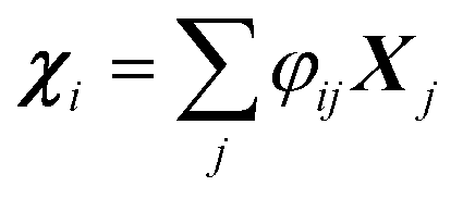 , where φij is the diagonalizing matrix of Mij such that
  . γi's are the relaxation rates of the individual Rouse modes and they are normalized by the relaxation rate due to the harmonic interactions γ = μζ. The coarse-grained Fokker–Planck equation for the probability density ρ(XCOM,t) in terms of the polymer's center of mass,
 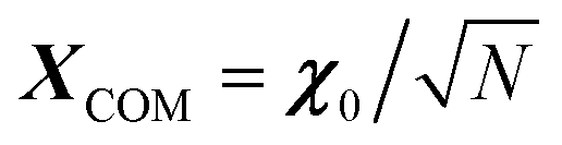 , is then obtained by integrating out the orientation vectors {pi(t)} and the other Rouse modes {χi(t); i ≠ 0} under a small gradient approximation as
 | (3) |
![[scr V, script letter V]](https://www.rsc.org/images/entities/char_e149.gif) and diffusive coefficient
and diffusive coefficient ![[scr D, script letter D]](https://www.rsc.org/images/entities/char_e523.gif) are functions of XCOM and are given by
are functions of XCOM and are given by | (4) |
 | (5) |
 | (6) |
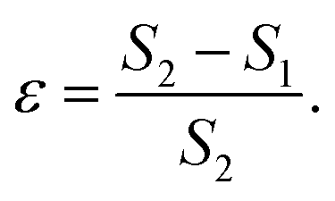
One can see in eqn (4) that the diffusivity of the polymer is enhanced due to activity compared to its all-passive counterpart (in which case the effective diffusivity would have been D/N) and the enhancement is proportional to the fraction S2 of active monomers in the polymer. The effective drift is generated by the gradient of the swim force squared, and is otherwise absent in passive or even constant activity systems. The steady state density of the center of mass of the polymer chain can now be calculated using the zero flux condition in (3) and the fact that 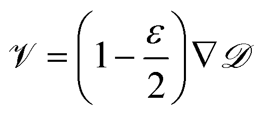 , where
 | (7) |
In particular, we obtain-
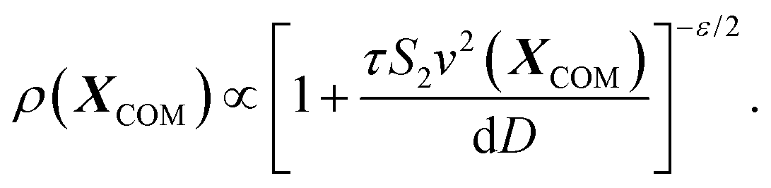 | (8) |
This tells us that the localization of polymers in response to activity is governed by the exponent ε, which encapsulates the competition between the effective drift, which causes the directed motion toward high activity regions, and effective diffusion, which tends to displace the polymer from its residing place. In particular, it is the sign of ε (or S2 − S1) that determines whether a polymer prefers to localize in high or low activity regions. For ε < 0, the density profile grows with the activity profile leading to preferential accumulation in high activity regions which is known as chemotaxis, while for ε > 0, the polymers accumulate in regions of low activity, leading to anti-chemotaxis.
Fig. 2 shows the steady state density profiles of various configurations of polymers for chain lengths N = 6 and N = 18, in an environment with a sinusoidal fuel concentration. Let us first consider the density distribution of polymers with a single active monomer compared to that with all monomers active. A polymer with only an end active monomer shows stronger accumulation in high activity regions compared to a polymer composed uniquely by active units. However, if the active monomer is located in the interior of the chain, the polymer's localization is weaker than an all-active polymer. This can be explained by the value of the exponent ε, which as mentioned before determines the location and effectiveness of the preferential accumulation. Precisely, the more negative is the value of ε, the more efficient is the accumulation of polymer in high activity regions. Therefore, by evaluating the values of ε (eqn (7)), we see that |εend| > |εall| > |εinterior| which supports the results presented in Fig. 2, which holds good independent of the polymer length, as can be seen from the results for N = 18 in Fig. 2.
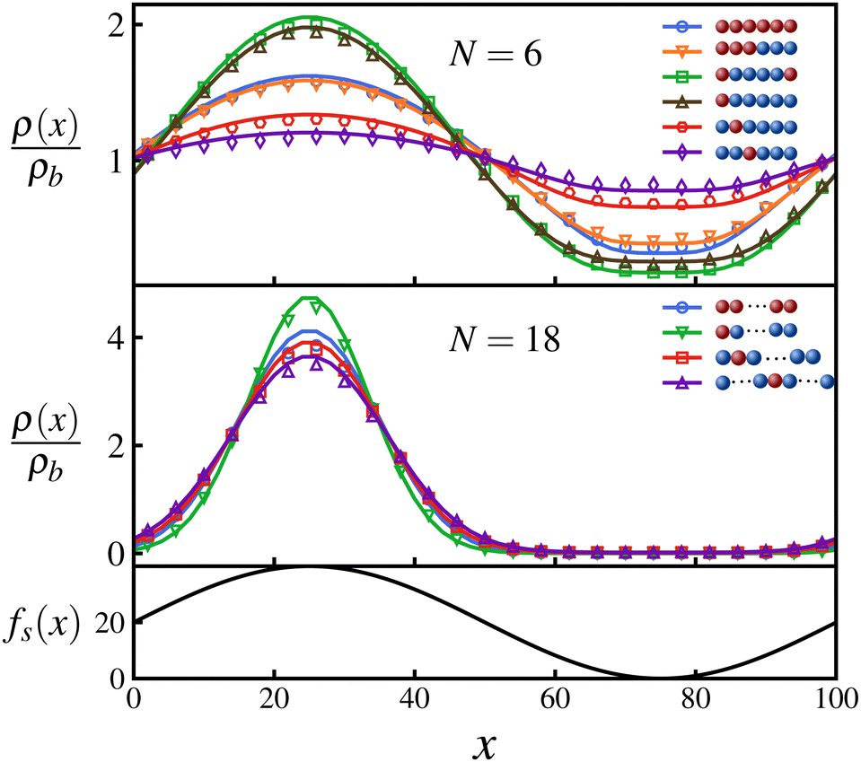 | ||
Fig. 2 The steady state density profiles for various configurations of a polymer with chain length N = 6 and N = 18 for ζ = 8, Dr = 5, μ = 1, and D = 1 in a box of length L = 100 that has a sinusoidally varying activity profile in the x-direction: 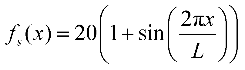 as depicted. The densities are normalized by ρb = 1/L. The solid lines represent analytical predictions and the symbols represent Langevin dynamics simulation results. as depicted. The densities are normalized by ρb = 1/L. The solid lines represent analytical predictions and the symbols represent Langevin dynamics simulation results. | ||
The limit N ≫ 1 can be considered analytically for selected configurations of chains with one active monomer. In this case the summations in eqn (5) can be transformed into integrals leading to closed analytic expressions as shown in the ESI.† In particular we obtain for ε:
 | (9) |
Using the symmetry of the eigenfunctions of the connectivity matrix for the linear chain (see ESI†) we draw some further general conclusions about the role of the position of the active monomers inside the chain: Consider polymers that have a symmetric distribution of active monomers along the chain, e.g., a polymer with both terminal monomers active, and their corresponding antisymmetric polymers in which the active monomers are present in only one of half of the chain, e.g., for the above mentioned case is a polymer chain with only one end monomer active. Using the fact that the absolute values of the elements of the eigenvectors form a palindromic set, we can show that the values of S1 and S2 (eqn (5)) for a symmetric polymer are twice of those of its corresponding antisymmetric polymer. This leads to the same epsilon value (eqn (7)) for both cases and as a result, their steady state densities differ only marginally due to the difference in the pre-factor in eqn (8), as can be seen in Fig. 2. This further emphasizes the fact that accumulative behaviour is largely determined by ε and shows that such a pair of symmetric–antisymmetric polymers have similar localization with respect to inhomogeneous activity.
Therefore, limiting our focus to polymers with just one or all monomers active, we construct in Fig. 3 a state diagram of the accumulation behavior of hybrid polymers. In particular, we consider polymers with different chain lengths N and three different configuration: active end monomer active, active central monomer active, and all monomers active. We observe that the switch from accumulation in lower activity regions to higher activity regions, for a given set of parameter values (ζ, μ, τ), can be achieved not only by increasing the chain length or varying the connectivity matrix as reported in ref. 41 but also by altering the number and positions of the active monomers within the polymer. Note that when all the monomers are active (αi = 1 for all i), the expression for the steady state density simplifies to the one presented in ref. 41 for polymers made up of Active Ornstein Uhlenbeck particles (AOUP's).71,72 This illustrates that the accumulative behavior of polymers is not dependent on the specific model of active particles considered. Our findings remain robust for semiflexible polymers with small bending stiffness. For a detailed study on the effect of bending interactions, one can refer the ESI.†
 | ||
| Fig. 3 Scatter plot for ε which indicates the location and degree of preferential accumulation for three distinct configuration of polymers of various chain length. Values of ε obtained analytically for the set of parameters mentioned in Fig. 2. As mentioned in the main text, ε < 0 on the colorbar indicates accumulation in high activity regions, and those greater than zero represent low-activity accumulation. | ||
Though eqn (8) gives us the steady state accumulation of various polymer chains, it does not give any insights into their dynamic behaviour, for example how fast do they get to the regions of high fuel concentration. In this direction, we solve for the mean first passage time (MFPT) T(x), x being the initial position of the polymer's center of mass, the equation for which is obtained using the coarse-grained Fokker–Planck equation as68
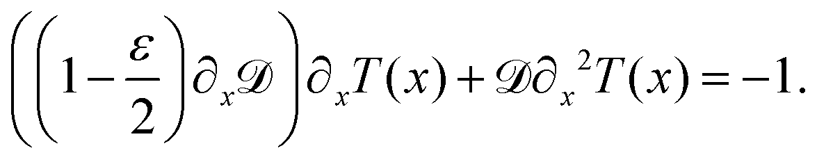 | (10) |
Setting tm = T(50) for a box of length L = 100, we calculate the average time taken by a polymer to reach the location of highest activity by imposing absorbing boundary conditions.68 The results for the mean first passage time for various polymer configurations are presented in Fig. 4. For a polymer with all monomers active, the MFPT decreases as we increase the number of monomers, becoming nearly independent of the chain length for N > 10. However, other polymers with one or two monomers active take longer to reach the region of highest activity. As can be evinced from Fig. 4, the MFPT of polymers with a single active monomer varies depending on the position of the latter along the chain, reaching the minimum value when the active monomer is an end monomer. Furthermore, in contrast to the previously discussed accumulation behavior, Fig. 4 shows that introducing a further active monomer in a symmetric position compared to a preexisting one (as shown by the green and red solid lines in Fig. 4) has a tangible impact on the MFPT. In particular, the configuration with two monomers (red lines) is much faster compared to the other (green line). These results suggest that increasing the number of active units within a polymer decreases its MFPT.
 | ||
| Fig. 4 The mean first passage time taken by a polymer to travel to the most active location starting from x = L/2 vs. the chain length of the polymer for four different configurations (other parameters are same as those specified in Fig. 2). The solid lines are theoretical predictions while the symbols are from Langevin dynamics simulations. | ||
Constructing a qualitative state diagram that encapsulates both the agility (defined as the inverse of MFPT) and the preferential accumulation behavior of polymers in Fig. 5, we get a comprehensive picture regarding hybrid polymers in chemical gradients. There seems to be no correlation between preferential accumulation and the mean first passage time of the polymers. We can therefore have polymers ranging from those that accumulate in high activity regions but are slow getting there (like long polymers (N > 10) with a sole interior monomer active) to those that are fast in getting to the high active regions but do not prefer to localize there (like relatively short polymers (N = 4) with all monomers active).
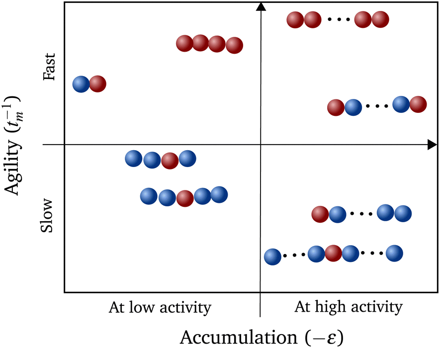 | ||
| Fig. 5 A qualitative state diagram that illustrates the two studied properties of various polymers: (i) location of accumulation on the x-axis – by taking the negative of ε and (ii) mean first passage time of polymers to reach the location of highest activity tm. | ||
From our studies, we can therefore suggest strategies for polymerization that leads to (i) maximum accumulation and (ii) fastest motion, for a given N. A polymer with both terminal monomers active would result in the former while the one with all units active would be the fastest. This information may shed light onto the evolutionary development of important biopolymers like actin73,74 and tubulin,75 even though the form of activity at these length scales are different. The best strategy required for the function of the biopolymer can still be constructed by altering the number and position of the active units within the polymer. Similar self-localization of symmetric and corresponding anti-symmetric polymers can also be an indicator of introduction of asymmetry in biopolymers during evolution to yield an energy efficient directed transport.
The resulting directed transport in our work is an emergent property. While one could explicitly couple particle orientation to the local activity gradient, dependent on the specific activity mechanism, this would introduce an additional effect beyond the one in our study. We have also focused on polymers of fixed lengths. The incorporation of polymerization and depolymerization into a dynamical model is left for a future work. Our findings can also be coupled with existing studies on polymerization induced phase separation to study the formation and behaviour of active cell organelles76 in future works.
Data availability
The code and primary data can be found at https://zenodo.org/records/14825768 with https://doi.org/10.5281/zenodo.14825768.Conflicts of interest
There are no conflicts to declare.Acknowledgements
A. S. acknowledges support by the Deutsche Forschungsgemeinschaft (DFG, German Research Foundation) within Project No. SH 1275/5-1. J. U. S. was supported by the DFG under Germany's Excellence Strategy – EXC 2068 – 390729961– Cluster of Excellence Physics of Life of TU Dresden. S. R. acknowledges support by the Deutscher Akademischer Austauschdienst (DAAD) – Funding ID-57693453.Notes and references
- F. Müller, Ecol. Modell., 1998, 108, 3–21 CrossRef.
- T. M. Keenan and A. Folch, Lab Chip, 2008, 8, 34–57 RSC.
- M. Almonacid, W. W. Ahmed, M. Bussonnier, P. Mailly, T. Betz, R. Voituriez, N. S. Gov and M.-H. Verlhac, Nat. Cell Biol., 2015, 17, 470–479 CrossRef CAS PubMed.
- M. Guthold, X. Zhu, C. Rivetti, G. Yang, N. H. Thomson, S. Kasas, H. G. Hansma, B. Smith, P. K. Hansma and C. Bustamante, Biophys. J., 1999, 77, 2284–2294 CrossRef CAS PubMed.
- B. Alberts, A. Johnson, J. Lewis, M. Raff, K. Roberts and P. Walter, Bray D. Cell movements: from molecules to motility, Garland Science, 2nd edn, 2000 Search PubMed.
- A. Javer, Z. Long, E. Nugent, M. Grisi, K. Siriwatwetchakul, K. D. Dorfman, P. Cicuta and M. Cosentino Lagomarsino, Nat. Commun., 2013, 4, 3003 CrossRef PubMed.
- S. C. Weber, A. J. Spakowitz and J. A. Theriot, Proc. Natl. Acad. Sci. U. S. A., 2012, 109, 7338–7343 CrossRef CAS PubMed.
- A. Zidovska, D. A. Weitz and T. J. Mitchison, Proc. Natl. Acad. Sci. U. S. A., 2013, 110, 15555–15560 CrossRef CAS.
- M. Di Pierro, D. A. Potoyan, P. G. Wolynes and J. N. Onuchic, Proc. Natl. Acad. Sci. U. S. A., 2018, 115, 7753–7758 CrossRef CAS PubMed.
- S. F. Banani, H. O. Lee, A. A. Hyman and M. K. Rosen, Nat. Rev. Mol. Cell Biol., 2017, 18, 285–298 CrossRef CAS.
- J.-U. Sommer, H. Merlitz and H. Schiessel, Macromolecules, 2022, 55, 4841–4851 CrossRef CAS.
- S. Ramaswamy, Annu. Rev. Condens. Matter Phys., 2010, 1, 323–345 CrossRef.
- S. Ramaswamy, J. Stat. Mech.: Theory Exp., 2017, 2017, 054002 CrossRef.
- G. De Magistris and D. Marenduzzo, Phys. A, 2015, 418, 65–77 CrossRef.
- É. Fodor, C. Nardini, M. E. Cates, J. Tailleur, P. Visco and F. Van Wijland, Phys. Rev. Lett., 2016, 117, 038103 CrossRef PubMed.
- G. Gompper, R. G. Winkler, T. Speck, A. Solon, C. Nardini, F. Peruani, H. Löwen, R. Golestanian, U. B. Kaupp and L. Alvarez, et al. , J. Phys.: Condens. Matter, 2020, 32, 193001 CrossRef CAS PubMed.
- F. Jülicher, S. W. Grill and G. Salbreux, Rep. Prog. Phys., 2018, 81, 076601 CrossRef PubMed.
- M. C. Marchetti, J.-F. Joanny, S. Ramaswamy, T. B. Liverpool, J. Prost, M. Rao and R. A. Simha, Rev. Mod. Phys., 2013, 85, 1143–1189 CrossRef CAS.
- C. P. Brangwynne, G. H. Koenderink, F. C. MacKintosh and D. A. Weitz, J. Cell Biol., 2008, 183, 583–587 CrossRef CAS PubMed.
- W. Lu, M. Winding, M. Lakonishok, J. Wildonger and V. I. Gelfand, Proc. Natl. Acad. Sci. U. S. A., 2016, 113, E4995–E5004 CAS.
- A. Ravichandran, G. A. Vliegenthart, G. Saggiorato, T. Auth and G. Gompper, Biophys. J., 2017, 113, 1121–1132 CrossRef CAS PubMed.
- C. A. Weber, R. Suzuki, V. Schaller, I. S. Aranson, A. R. Bausch and E. Frey, Proc. Natl. Acad. Sci. U. S. A., 2015, 112, 10703–10707 CrossRef CAS PubMed.
- R. G. Winkler, J. Elgeti and G. Gompper, J. Phys. Soc. Jpn., 2017, 86, 101014 CrossRef.
- R. G. Winkler and G. Gompper, J. Chem. Phys., 2020, 153, 040901 CrossRef CAS PubMed.
- S. K. Anand and S. P. Singh, Phys. Rev. E, 2018, 98, 042501 CrossRef.
- R. E. Isele-Holder, J. Elgeti and G. Gompper, Soft Matter, 2015, 11, 7181–7190 RSC.
- C. A. Philipps, G. Gompper and R. G. Winkler, J. Chem. Phys., 2022, 157, 194904 CrossRef PubMed.
- E. Locatelli, V. Bianco and P. Malgaretti, Phys. Rev. Lett., 2021, 126, 097801 CrossRef CAS PubMed.
- A. Kaiser and H. Löwen, J. Chem. Phys., 2014, 141, 044903 CrossRef CAS PubMed.
- C. Zhang, C. Xie, W. Feng, H. Luo, Y. Liu and G. Jing, New J. Phys., 2023, 25, 043029 CrossRef.
- C. J. Anderson, G. Briand, O. Dauchot and A. Fernández-Nieves, Phys. Rev. E, 2022, 106, 064606 CrossRef CAS PubMed.
- J. Harder, C. Valeriani and A. Cacciuto, Phys. Rev. E, 2014, 90, 062312 CrossRef CAS PubMed.
- S. M. Mousavi, G. Gompper and R. G. Winkler, J. Chem. Phys., 2021, 155, 044902 CrossRef CAS PubMed.
- J. Shin, A. G. Cherstvy, W. K. Kim and R. Metzler, New J. Phys., 2015, 17, 113008 CrossRef.
- M. Foglino, E. Locatelli, C. Brackley, D. Michieletto, C. Likos and D. Marenduzzo, Soft Matter, 2019, 15, 5995–6005 RSC.
- V. Bianco, E. Locatelli and P. Malgaretti, Phys. Rev. Lett., 2018, 121, 217802 CrossRef CAS PubMed.
- L. Natali, L. Caprini and F. Cecconi, Soft Matter, 2020, 16, 2594–2604 RSC.
- J.-X. Li, S. Wu, L.-L. Hao, Q.-L. Lei and Y.-Q. Ma, Phys. Rev. Res., 2023, 5, 043064 CrossRef CAS.
- M.-B. Luo and Y.-F. Shen, Soft Matter, 2024, 20, 5113–5121 RSC.
- H. D. Vuijk, H. Merlitz, M. Lang, A. Sharma and J.-U. Sommer, Phys. Rev. Lett., 2021, 126, 208102 CrossRef CAS PubMed.
- P. L. Muzzeddu, A. Gambassi, J.-U. Sommer and A. Sharma, Phys. Rev. Lett., 2024, 133, 118102 CrossRef CAS PubMed.
- L. Caprini, U. M. B. Marconi, R. Wittmann and H. Löwen, Soft Matter, 2022, 18, 1412–1422 RSC.
- A. Wysocki, A. K. Dasanna and H. Rieger, New J. Phys., 2022, 24, 093013 CrossRef.
- J. R. Howse, R. A. Jones, A. J. Ryan, T. Gough, R. Vafabakhsh and R. Golestanian, Phys. Rev. Lett., 2007, 99, 048102 CrossRef PubMed.
- H. Löwen, Europhys. Lett., 2018, 121, 58001 CrossRef.
- J. Elgeti, R. G. Winkler and G. Gompper, Rep. Prog. Phys., 2015, 78, 056601 CrossRef CAS PubMed.
- C. Bechinger, R. Di Leonardo, H. Löwen, C. Reichhardt, G. Volpe and G. Volpe, Rev. Mod. Phys., 2016, 88, 045006 CrossRef.
- R. Dreyfus, J. Baudry, M. L. Roper, M. Fermigier, H. A. Stone and J. Bibette, Nature, 2005, 437, 862–865 CrossRef CAS PubMed.
- A. Najafi and R. Golestanian, Phys. Rev. E: Stat., Nonlinear, Soft Matter Phys., 2004, 69, 062901 CrossRef PubMed.
- H.-R. Jiang, N. Yoshinaga and M. Sano, Phys. Rev. Lett., 2010, 105, 268302 CrossRef PubMed.
- I. Theurkauff, C. Cottin-Bizonne, J. Palacci, C. Ybert and L. Bocquet, Phys. Rev. Lett., 2012, 108, 268303 CrossRef CAS PubMed.
- L. F. Valadares, Y.-G. Tao, N. S. Zacharia, V. Kitaev, F. Galembeck, R. Kapral and G. A. Ozin, Small, 2010, 6, 565–572 CrossRef CAS PubMed.
- M. J. Schnitzer, Phys. Rev. E, 1993, 48, 2553 CrossRef CAS PubMed.
- A. Sharma and J. M. Brader, Phys. Rev. E, 2017, 96, 032604 CrossRef CAS PubMed.
- H. C. Berg, E. coli in Motion, Springer, 2004 Search PubMed.
- M. Schnitzer, S. Block and H. Berg, Biology of the chemotactic response, 1990, vol. 46, pp. 15 Search PubMed.
- H. C. Berg, Random walks in biology, Princeton University Press, 1993 Search PubMed.
- I. R. Lapidus, J. Theor. Biol., 1980, 86, 91–103 CrossRef CAS PubMed.
- F. Peng, Y. Tu, J. C. Van Hest and D. A. Wilson, Angew. Chem., Int. Ed., 2015, 54, 11662–11665 CrossRef CAS PubMed.
- P. K. Ghosh, Y. Li, F. Marchesoni and F. Nori, Phys. Rev. E, 2015, 92, 012114 CrossRef PubMed.
- H. D. Vuijk, A. Sharma, D. Mondal, J.-U. Sommer and H. Merlitz, Phys. Rev. E, 2018, 97, 042612 CrossRef CAS PubMed.
- H. Merlitz, H. D. Vuijk, R. Wittmann, A. Sharma and J.-U. Sommer, PLoS One, 2020, 15, e0230873 CrossRef CAS PubMed.
- H. D. Vuijk, S. Klempahn, H. Merlitz, J.-U. Sommer and A. Sharma, Phys. Rev. E, 2022, 106, 014617 CrossRef CAS PubMed.
- P. L. Muzzeddu, H. D. Vuijk, H. Löwen, J.-U. Sommer and A. Sharma, J. Chem. Phys., 2022, 157, 134902 CrossRef CAS PubMed.
- P. L. Muzzeddu, É. Roldán, A. Gambassi and A. Sharma, EPL, 2023, 142, 67001 CrossRef CAS.
- B. Valecha, P. L. Muzzeddu, J.-U. Sommer and A. Sharma, arXiv, 2024, preprint, arXiv:2409.18703 DOI:10.48550/arXiv.2409.18703.
- J.-U. Sommer and A. Blumen, J. Phys. A: Math. Gen., 1995, 28, 6669 CrossRef CAS.
- C. W. Gardiner, Springer series in synergetics, 1985 Search PubMed.
- H. Risken, The Fokker–Planck Equation, 1996 Search PubMed.
- M. Doi, S. F. Edwards and S. F. Edwards, The theory of polymer dynamics, oxford university press, 1988, vol. 73 Search PubMed.
- D. Martin, J. O’Byrne, M. E. Cates, É. Fodor, C. Nardini, J. Tailleur and F. Van Wijland, Phys. Rev. E, 2021, 103, 032607 CrossRef CAS PubMed.
- L. Caprini and U. M. B. Marconi, Soft Matter, 2018, 14, 9044–9054 RSC.
- F. Straub, Stud. Inst. Med. Chem., Univ. Szeged, 1943, 3, 23–37 CAS.
- S. Y. Khaitlina, Biochemistry, 2014, 79, 917–927 CAS.
- E. Hamel and C. M. Lin, Biochemistry, 1984, 23, 4173–4184 CrossRef CAS PubMed.
- C. A. Weber, D. Zwicker, F. Jülicher and C. F. Lee, Rep. Prog. Phys., 2019, 82, 064601 CrossRef CAS PubMed.
Footnote |
| † Electronic supplementary information (ESI) available. See DOI: https://doi.org/10.1039/d4sm01357c |
| This journal is © The Royal Society of Chemistry 2025 |