
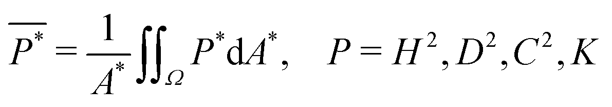
 Open Access Article
 This Open Access Article is licensed under a Creative Commons Attribution-Non Commercial 3.0 Unported Licence
Cholesteric liquid crystal roughness models: from statistical characterization to inverse engineering†
Ziheng
Wang
 ,
Phillip
Servio
and
Alejandro D.
Rey
*
,
Phillip
Servio
and
Alejandro D.
Rey
*
Department of Chemical Engineering, McGill University, 3610 University Street, Montréal, Québec H3A 2B2, Canada. E-mail: alejandro.rey@mcgill.ca
First published on 16th May 2025
Abstract
The surface geometry, particularly the curvature and roughness, play crucial roles in the functionalities of bio-compatible cholesteric liquid crystal (CLC) substrates. For example, experiments show increased alignment of hBMSCs (human bone-marrow-derived stromal cells) with larger curvature on a cylindrical manifold [Callens et al., Biomaterials, 2020, 232, 119739]. Previous studies on cholesteric liquid crystal surfaces have primarily focused on an elastic approach, which does not fully capture the anisotropic nature and multiscale wrinkling profiles. The objective of this research is to characterize the surface geometry of CLCs based on a generalized anisotropic anchoring model (the Rapini–Papoular model). In this paper, we propose both analytic approximations and direct numerical solutions for surface wrinkling, curvature profiles, and surface roughness characterization. We also explore the important limits of the Rapini–Papoular model, including lower bounds for the kurtosis and Willmore energy. The inverse problem offers an alternative approach to measuring the anchoring coefficients, which are difficult to determine experimentally. These findings suggest that surface anchoring is the key determinant of multiscale surface wrinkling patterns. This paper sheds light on the applications and functionalities of surface wrinkling patterns in liquid crystals and their solid analogues. Furthermore, this research incorporates a novel coordinate-free differential geometric approach and provides a general framework for studying dynamic properties and surface evolution.
1 Introduction
Synthetic and biological liquid crystals (LCs) are partially ordered materials formed by anisotropic components such as rod-like molecules, fibrils, and filaments which exhibit anisotropic viscoelastic properties.1–3 Being partially ordered in terms of position and orientation, LCs exhibit both solid (such as anisotropy) and liquid (such as fluidity) characteristics. The macroscopic orientation is denoted by a unit vector or director n(x) of cholesteric liquid crystals (CLCs) show chirality, which is characterized by the helix pitch P0, that satisfies n(x + P0) = n(x), that is, the spatial distance for a 2π rotation of the director field is P0.4–6 The chiral architecture is ubiquitous in biological materials,7–11 and was systematically studied by Bouligand. Synthetic and biological cholesteric liquid crystal analogues (CLCAs) are solids with the frozen-in structure of CLCs resulting from various solidification processes.12–17 As mentioned in more detail, below in this paper, we model and study surface roughness in CLCs for potential biomimetic functional surface applications while CLCAs and related nature's surfaces are the source of biological inspiration as well as geometric data for surface roughness.Some examples of biological CLCAs are the chitin fibres of the shimmering beetles’ exoskeleton,18–20 cellulosics of biological plywoods19,21,22 and collagens of human compact bones.19,23,24 Other important examples of CLCs and CLCAs analogues are DNA both in vivo and in vitro,10,25 viruses,26 spider silk,27,28 fibroblasts and osteoblasts.29,30
Fig. 1 summarizes the main objectives, key phenomena and modelling methods used in this paper. The middle schematic of Fig. 1 shows the surface wrinkling of flower petals, where the cellulosics form a Bouligand structure that is a source of inspiration and data for our surface geometry model for cholesteric liquid crystals. The surface morphology of these materials includes creasing, folding, ridges and wrinkling.31–36 For example, surface creasing can be found in swelling induced hydrogels37,38 and others.39–41 In biological membrane systems such as the Golgi apparatus,42 mitochondrion membranes43,44 and cortical tissues,45–47 surface folding and curvature distribution are key factors affecting biochemical functionalities.48 In this paper, we study the multiscale wrinkling profile driven by CLC surface anchoring. The two unique characteristics of multiscale CLC surface are: (1) the helix pitch P0 is in the scale of few micrometers, while the surface wrinkling is in the scale of nanometres.22,49–52 (2) The surface profile is periodic and tends to form egg-carton patterns.52–56 The two observations imply that the cause of the periodic nanowrinkling profile is not driven by elasticity, since an elastic model does not result in multiscale wrinkling patterns,57,58 and it cannot explain the P0-dependent periodicity. To answer those questions, we developed a theoretical framework, shown in Fig. 1 on the left column. Our previous works explain and validate that surface anchoring is the cause of CLC multiscale wrinkling patterns.22,49,50,53–55,59–63 Cheong et al. applied Cahn–Hoffman capillary vector approach to study LC fibre instability,64–68 which is further generalized and combined with an elastic model to study the elastic CLC membrane wrinkling.22,49,50 Wang et al. studied the 3D structure of the Bouligand structure and successfully obtained egg-carton surfaces.53–55 These previous works we based on low order contributions to the anchoring energies, while the effect of higher order contributions to anisotropic surface energy is the key focus of this paper.
 | ||
| Fig. 1 Graphical summary of the goals, key phenomena and modelling methods of this paper. The blue arrows connect theoretical development of CLC surfaces (physics), and pink arrows connect surface roughness development (experimental data). Centre schematic: this paper is motivated by bio-inspired multiscale wrinkling patterns observed in nature, as in flower petals. Left schematic: we develop a generalized cholesteric liquid crystal shape equation to predict surface roughness and wrinkling as in nature (left upper arrow). We briefly summarize our previous work in Sections 2.1 and 2.2. In these sections, the anisotropic material surface properties of interest are the anchoring coefficients. Right schematic: in this paper we generalize the traditional study and characterization of metal surfaces roughness as inspired by nature (right middle arrow) to describe LCs, considering that CLC surfaces are soft. The quantities of interest in this section are roughness parameters. We study the forward (prediction) problem in Sections 3.1 and 3.2. In the forward problem, we apply the method we developed in previous literature22,49,50,53–55,59–63 to study the surface roughness. In Section 3.3, we study the inverse problem by solving the physics from measured biological surface roughness parameters. The middle figure is reproduced from ref. 69 with permission from Royal Society of Chemistry (2017). | ||
The right schematic of Fig. 1 shows the domain of surface roughness (or smoothness) for hard material surfaces such as metallic. The surface roughness of hard surface plays an important role in engineering and manufacturing. For example, surface roughness is widely studied to investigate its influence in fluid mechanics,70–72 electrical properties,73,74 optical properties,75,76 wettability,77,78 friction and adhesion,79,80 heat distribution,81 interfacial corrosion,82,83 and physiochemical process.84,85 However, similar theoretical and/or experimental studies in soft surfaces are not well established, despite the fact that soft surface roughness are critical to its multifunctionality. For example, the roughness of an endoplasmic reticulum determines different tasks in biology. A smooth endoplasmic reticulum synthesizes lipids and phospholipids,86,87 while a rough endoplasmic reticulum is a factory for secreted proteins.88,89 Traditional approaches to studying hard surface roughness rely on statistics, because the hard surfaces are in general non-analytic and we cannot take mathematical derivatives on the surface. The most useful surface roughness tools include parametric methods and functional methods. Parametric methods calculate higher-order moments of the surface profile, where the second-order (root mean square, Sq), third-order (skewness, Rsk) and fourth-order (kurtosis, Rku) moments measure the deviation, asymmetry, and tailedness of surface profile distribution, respectively. Functional methods include autocorrelation function and power spectral density, which are important features of a periodic surface.84 In this paper, besides adapting traditional approaches from hard surface roughness methods, we also propose a new curvature-based method to support the surface roughness theory for anisotropic soft matter. An advantage of soft surface is that the curvature can be an indicator for surface roughness. We demonstrate that the curvature-based method is equivalent to the membrane geometric energy (such as Willmore energy,90–92 Helfrich energy93–95) and has been widely studied in the theory of geometric flows.96,97 Other methods such as fractal methods can be used to study the self-similar structure in a nested network, with the advantage of analyzing scale-independent hierarchical structures.98–100
In partial summary, the left schematic of Fig. 1 summarizes the physics, theory and computational platform for CLC surfaces, while the right column demonstrates the surface roughness characterization methods widely used for hard surfaces that, as we show here, can be tailored to soft surfaces such as those CLCs. In Sections 3.1 and 3.2 of this paper, we discuss the forward engineering problem by applying the LC surface theory and shape equations we developed in previous papers,22,55,101 to predict and characterize the surface roughness of LC surfaces. In Section 3.3, we study the inverse surface roughness problem, by using the data from biological surface roughness to reconstruct the LC surface physics (determination of anchoring coefficients).
This inverse problem (Section 3.3) is of great significance to LC material property characterization, because the data of surface roughness is usually much easier to obtain than actual LC anchoring coefficients. For example, methods of measuring surface profile are usually direct methods. Traditional methods include mechanical stylus method,102 light sectioning method,103 scattering method,104,105 scanning electron microscopy,106,107 scanning probe microscopy,108,109 machine vision method such as Fourier transform110 or wavelet transform111etc. The measurement of anchoring coefficient μ2, however, is through indirect method which involves calculating a deviation orientation angle.112,113 Most experimental approaches require the evaluation of a certain twist or deviation angle ϕ, or even higher-order derivatives of ϕ. For example, μ2 can be calculated by measuring the threshold voltage of Fréedericksz transition Vth, the Franck constants Ki (i = 1, 2, 3, 24), and the dielectric susceptibility anisotropy Δχ such that  . μ2 can also be evaluated with a rubbed nano-sized groove surface such that μ2 = f(ϕ, Ki),114 or with a spectroscopic ellipsometry approach by solving a PDE dependent on μ2, ϕ,
  and
and  .115 The calculation of the deviation angle ϕ is usually hypersensitive to noise since it is based on derivatives. On the other hand, the measurement of surface roughness parameters involves taking integrals and is therefore less affected by noise. For example, if the measured surface is disturbed by δW, where W is the noise following a standard normal distribution
  and δ is a small amplitude. We can show that the expected value of the root mean square deviates from the model by
  . It demonstrates that the higher moment methods discussed in this paper are barely affected by the random noise. Another advantage of the new method is that traditional approaches of measuring the anchoring coefficient only give the value of low-order components μ2 (see Section 2) while the inverse problem engineering can provide the values of higher-order contributions ri (see Section 3.3) simply by taking higher-order moments.
In summary, the objectives of this paper are as follows:
1. To formulate the generalized governing liquid crystal shape equations that describes the complex surface wrinkling patterns of CLCs, observed in nature;
2. To formulate, execute and validate numerical calculations and generalize high fidelity analytic solutions to the governing nonlinear shape equations that predict multiscale, complex surface roughness in CLCs, as observed in nature;
3. To predict key surface geometry characteristics such as standard (mean, Gaussian) and novel (Casorati, geometric shape index) curvatures and surface roughness statistics (kurtosis, skewness, correlations) of CLCs using biological surface geometry in-put data, including plant leaves and fish skin;
4. To develop and solve the inverse engineering problem in LC surface roughness and use validated results to predict all anchoring coefficients of CLCs that define the surface free energy.
The outline of this paper is as follows. In Section 2.1, we derive the governing shape equation, where the surface profile h is described by a nonlinear partial differential equation. In Section 2.2, we linearize the nonlinear shape equation PDE under a small-wrinkling assumption and solve the PDE with a spectral method. In Section 2.3, we introduce the concepts and definitions of the surface roughness parameters that will be discussed in Section 3; the concepts are summarized in Table 2. The results will be characterized and discussed in Section 3. In Section 3.1, we study the direct numerical solution of the nonlinear shape equation PDE and conclude that small-wrinkling approximation is of high fidelity. In Section 3.2, we study the surface curvatures (Section 3.2.1), higher-order moments (Section 3.2.2), and autocorrelation function (Section 3.2.3), which are obtained from the second derivative, the surface integral, and the self-convolution of the surface profile, respectively. In Section 3.3, we study the inverse engineering problem, and propose an application to find anchoring material properties. The main results, their novelty and significance and the contributions to surface roughness in cholesteric liquid crystals and anisotropic soft matter are presented in the Conclusions. All mathematical details are presented in the ESI.†
The scope of this paper is restricted to an equilibrium cholesteric liquid crystal surface described by an orientation vector or director field. Higher-order tensor models,116–119 time-dependent phenomena,120–124 dissipation,125 dynamics,126–132 tangential forces and flows,133–139 and bulk-surface couplings,101,140 are not included here and are left to future work. Below we use interchangeably biological and nature's surfaces.
2 Methods
In Section 2.1 we introduce the generalized governing shape equation for CLCs that includes higher-order harmonics to the anisotropic surface energy and extends our previously formulated liquid crystal shape equations.55,59,60 In Section 2.2 we obtain a very useful approximate analytical solution to the generalized nonlinear liquid crystal shape equation to predict surface shapes under small amplitude conditions. The analytical solution is crucial to validate our computational methods and to shed light on shape-generating mechanisms.2.1 Generalized governing liquid crystal shape equations
The anisotropic surface energy density γ of a cholesteric liquid crystal is the sum of an isotropic surface tension γ0 and anisotropic contributions. The surface energy density γ is calculated by the generalized Rapini–Papoular model of a polynomial with order 2m:53,55,59,60,63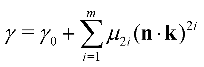 | (1) |
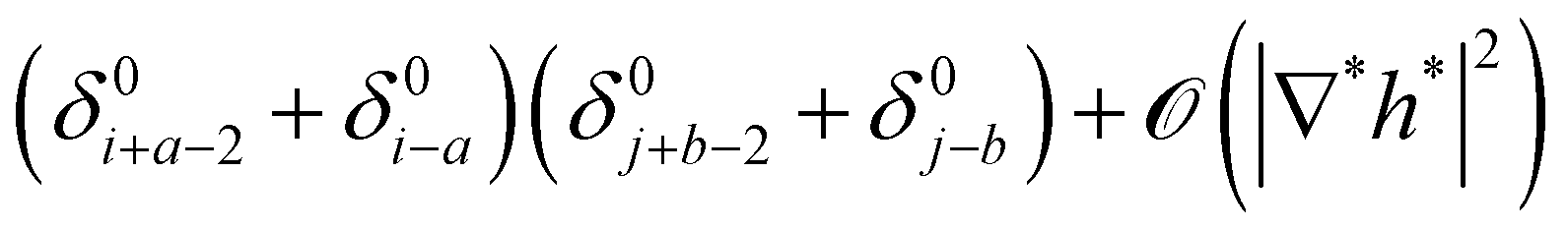
 . The second symmetry implies that the surface energy density is invariant to different conventions of surface unit normal. However, we pay attention to the direction of k, since k and −k alter the sign of curvature definitions. The details concerning this issue have been previously discussed in literature.62 In our previous work on nanowrinkling of cholesteric surfaces we study cases with m = 1, 2.22,49,53,55,60 The anchoring coefficients of eqn (1) are restricted by γ > 0 under all circumstances, and the details are given in Section S2 of ESI.†
The Cahn–Hoffman capillary vector ξ is a useful tool in studying direction-dependent materials since it incorporates interfacial anisotropy into the model.141–143 The decomposition of Cahn–Hoffman capillary vector ξ results in a tangential component ξ‖ and a normal component ξ⊥.66,144 The details of Cahn–Hoffman capillary vector approach are included in Section S1 of ESI.†
 | (2) |
 | (3) |
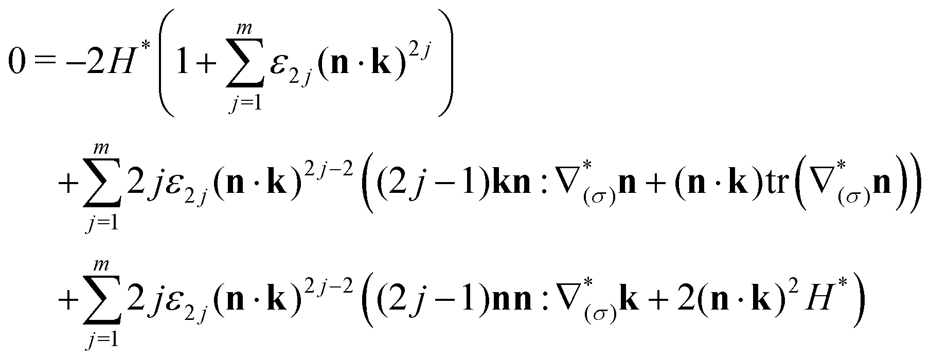
![[scr D, script letter D]](https://www.rsc.org/images/entities/char_e523.gif) p demonstrates three non-vanishing effects: an area dilation of p (dilation pressure), a director n effect (director pressure) and a k-rotation (rotation pressure) effect. The expansions of principal capillary pressures in the generalized Rapini-Rapoular model are (mathematical details are given in Section S1 of ESI†)
p demonstrates three non-vanishing effects: an area dilation of p (dilation pressure), a director n effect (director pressure) and a k-rotation (rotation pressure) effect. The expansions of principal capillary pressures in the generalized Rapini-Rapoular model are (mathematical details are given in Section S1 of ESI†)| Dilation pressure = 2Hγ | (4) |
 | (5) |
 | (6) |
 | (7) |
 | (8) |
2.2 Linear model of surface wrinkling
Observations show that surface wrinkling in nature is usually in the scale of nanometres, while the helix pitch is in the range of micrometers,22,49–52 indicating the presence of a small parameter in the shape eqn (7). Hence under a small wrinkling approximation (|ε2j| ≪ 1), the shape eqn (7) can be linearized. The simplified eqn (7) is solvable by the spectral method, which gives the solution as a linear combination of distinct cos![[thin space (1/6-em)]](https://www.rsc.org/images/entities/char_2009.gif) 2πωx*x*cos2πωy*y* fundamental wrinkling modes. We denote those wrinkling modes as 〈ωx*, ωy*〉 for simplicity in this paper and in the ESI.† The linear solution under the Monge parametrization h* = h*(x*, y*) can be written as (mathematical details are included in Sections S3 and S4 of ESI†):
2πωx*x*cos2πωy*y* fundamental wrinkling modes. We denote those wrinkling modes as 〈ωx*, ωy*〉 for simplicity in this paper and in the ESI.† The linear solution under the Monge parametrization h* = h*(x*, y*) can be written as (mathematical details are included in Sections S3 and S4 of ESI†): | (9) |
 to a surface profile of zero mean. wx* and wy* are the wrinkling vectors along the coordinates x* and y* coordinates:
 | (10) |
The calculation details and numerical methods of Q-matrices are given in the ESI.†

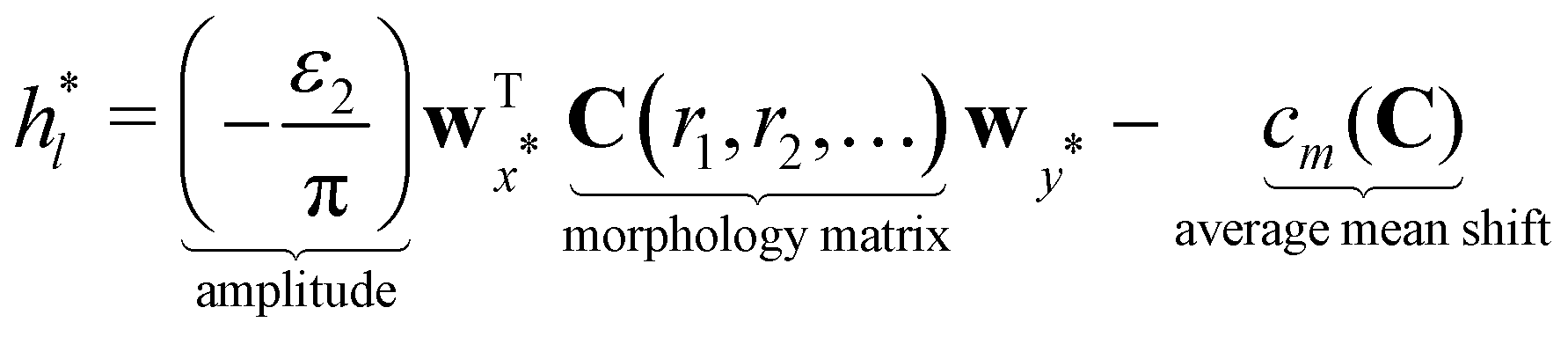
Eqn (7) shows a translational symmetry h* → h* + c, and as above-mentioned the constant c is chosen such that the average mean value of h* profile is zero, which furthers simplifies the calculation of the surface roughness discussed in Section 3. In conclusion, the linear solution  can be compactly rewritten as:
 | (11) |
 is the summation of the weighted Q-matrices and is only dependent to the anchoring ratios rj. In eqn (11), the amplitude is only dependent to the second order anchoring coefficient ε2; the average mean shift is a constant determined by the morphology matrix C; the morphology of the wrinkling profile is controlled by the anchoring coefficient ratios r1, r2, … Fig. 2(a) shows a representative visualization of constant Q-matrices (see ESI†). Each element in the matrix represents a distinct wrinkling mode. Fig. 2(b) is the wrinkling mode 〈1, 2〉, which corresponds to the second row and third column (dark red) of each Q-matrix.
 | ||
| Fig. 2 (a) Visualization of Q*-matrix where the colour represents the weight of each wrinkling modes in a Q-matrix. The dash line encircles the location of previous Q*-matrix. The index (i, j) of each Q*-matrix corresponds to a unique wrinkling mode with ωx* = (i − 1) and ωy* = (j − 1). For example, the (2, 3) component of each Q*-matrix represents a wrinkling mode cos2π(2 − 1)x*cos2π(3 − 1)y* described by (b). | ||
All elements in a Q-matrix are non-negative, hence Q-matrices can be normalized by  such that each element represents the weight of the total elements. In Fig. 2(a), the dominating three principal wrinkling modes for each matrix are (1) biaxial wrinkling 〈1, 2〉, shown in dark red colour; (2) equibiaxial wrinkling 〈2, 2〉, shown in green-cyan colour and (3) uniaxial wrinkling 〈2, 0〉, shown in yellow colour. The other wrinkling modes, corresponding to higher order harmonic waves, contribute much less than the three principal modes. This pattern remains the same from
  to
to  . The linear combination of
  with coefficient of rj−1 (which is C-matrix) shows an anchoring ratio-independent feature of three dominating wrinkling modes: 〈1, 2〉, 〈2, 2〉, and 〈2, 0〉.
In this paper, we study the 6th-order Rapini-Rapoular model numerically and expand the results to a generalized 2mth-order model. In a 6th-order anchoring mode, the characteristic lines in the parametric space (r1, r2) are shown in Fig. 3. These characteristic lines, and the vanishing modes are summarized in Table 1. r1 and r2 are constrained by ε2 since a thermodynamic stability requires γ* > 0. The details are discussed in Section S2 of ESI.†
 | ||
| Fig. 3 (a) Characteristic lines in the parametric space (r1, r2); (b) expansion around negative r1 values. Along each characteristic line, one wrinkling mode vanishes. | ||
| Characteristic lines | Colour | Vanishing modes | Category |
|---|---|---|---|
|
Red | 〈2,0〉 + 〈1,2〉 | Uniaxial + biaxial |
|
Black | 〈4,0〉 + 〈1,4〉 | Uniaxial + biaxial |

|
Blue | 〈2,2〉 | Equibiaxial |

|
Magenta | 〈4,4〉 | Equibiaxial |
|
Green | 〈2,4〉 + 〈4,2〉 | Biaxial |

|
Cyan | 〈3,2〉 | Biaxial |

|
Purple | 〈3,4〉 | Biaxial |
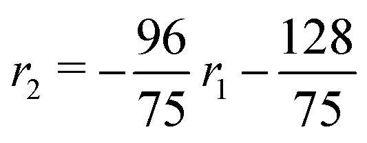
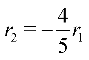
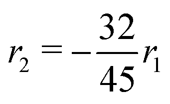
The wrinkling modes 〈ωx*, ωy*〉 can be categorized into three groups: (1) uniaxial wrinkling (if ωx*ωy* = 0); (2) equibiaxial wrinkling (if ωx*ωy* ≠ 0 and ωx* = ωy*); or (3) biaxial wrinkling (if ωx*ωy* ≠ 0 and ωx* ≠ ωy*). A pure uniaxial wrinkling mode represents a developable surface where Gaussian curvature vanishes everywhere. A pure equibiaxial wrinkling mode represents an ideal egg-carton surface, where x* and y*-axes are symmetric. In nature, most surfaces are biaxial. In Table 1, if r2 = −(4/5)r1, the uniaxial mode 〈4, 0〉 and biaxial mode 〈1, 4〉 vanish, and the surface is a linear combination of 19 different wrinkling modes (see Section S4 of ESI†).
2.3 Surface roughness characterization
In this section, we present and discuss the definitions for all the surface roughness characterizations and parameters studied in this paper and summarize them into Table 2. In the following, we categorize the surface roughness into three methods: (1) curvature; (2) higher-order moments; (3) autocorrelation. Results using the three methods will be discussed in Sections 3.2.1, 3.2.2 and 3.2.3 respectively.| Surface roughness parameter | Nomenclature | Range | Section | Surface profile (h*) | Significance |
|---|---|---|---|---|---|
| Average magnitude of curvature |

|
≥0 | 3.2.1 | Twice differentiable | Total Willmore/Helfrich energy |
| Root mean square | Sq | ≥0 | 3.2.2 | No requirement | Standard deviation |
| Skewness | Rsk | ![[Doublestruck R]](https://www.rsc.org/images/entities/char_e175.gif) |
3.2.2 | No requirement | Degree of bias of the roughness profile |
| Kurtosis | Rku | ≥0 | 3.2.2 | No requirement | Sharpness of roughness profile |
| Autocorrelation function | acf | 1 ≥ acf ≥ −1 | 3.2.3 | No requirement | Surface self-convolution |
| Autocorrelation length | Sal | 1 > Sal > 0 or ∅ | 3.2.3 | No requirement | High/low frequency dominated |
Next we discuss the definitions and nomenclature introduced in Table 2.
1. The surface curvatures are defined by the components of curvature tensor  . The usual curvatures are mean curvature H* = trB/2 and the Gaussian curvature K* = detB. The deviatoric curvature is
  (deviation from a sphere) and the Casorati curvature
 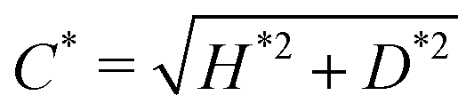 (deviation from a flat plane). The dimensionless shape parameter S = (2/π)arctan(H*/D*) is a normalized shape index that takes value between −1 to +1. The three primitive shapes are sphere (S = ±1), cylinder (S = ±0.5) and saddle (S = 0). The signs correspond to concave up or down. These curvatures are further discussed in our previous work145–147 but we emphasize that the (C, S) description separates shape and curvedness properties while the standard (H, K) geometric formulation co-mingles shapes and curvedness but if the main focus is shape description or curvedness description then the (C, S) methodology is preferable.
All the curvatures defined previously can also be written in terms of two principal curvatures: a larger curvature  and a smaller curvature
  .
.
 | (12) |
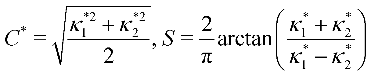 | (13) |
Since curvature is a quantity defined on a single point, we introduce an average quantity  to measure the average curvature magnitude with respect to the P*-curvature by
 | (14) |
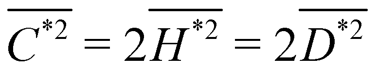 and
and  as restricted by the Gauss–Bonnet theorem.148–150 Hence, minimizing
  is equivalent to minimizing
  (Helfrich elastic energy93–95) or
  (Willmore energy90–92). In the following content, to investigate the average curvature, we only need to consider the mean curvature
  . The average magnitude of mean curvature
  can be calculated with the linear approximation of the surface profile in eqn (11). For example, the mean curvature can be calculated with
  . The average magnitude of the mean curvature is therefore
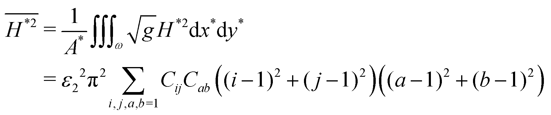 | (15) |
 | (16) |
 where the anchoring ratios (r1, r2, …) are encapsulated inside the Cij-matrices.
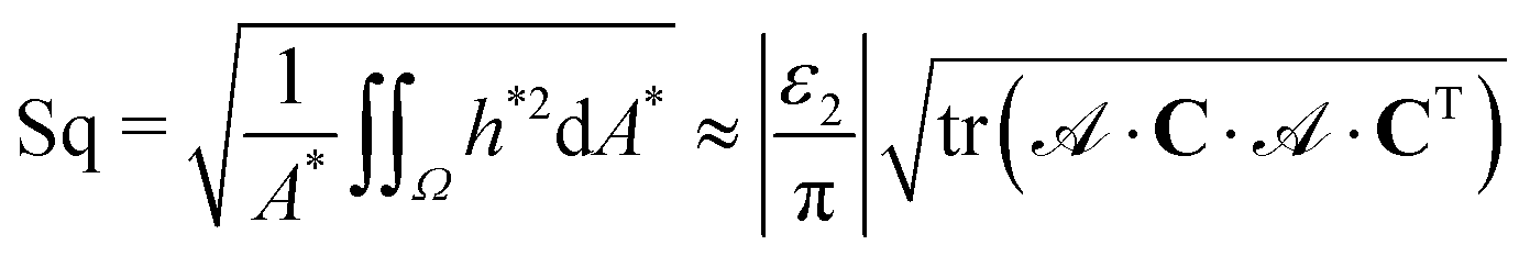
2. The average curvature magnitude  is defined only if the surface is smooth. A more general approach is to consider the higher-order moments. The first-order moment (mean), second-order moment (root mean square), third-order moment (skewness) and fourth-order moment (kurtosis) are the most applicable features of a surface profile. The first-order moment is zero since it is the condition to determine cm value in eqn (11). For a mean-free surface profile, the root mean square (Sq), surface skewness (Rsk) and kurtosis (Rku) are defined by the following equations (details are included in Section S6 of ESI†):
 | (17) |
 | (18) |
 | (19) |
 | (20) |
3. The method of higher-order moments focuses on the h-direction, while the autocorrelation length takes the information along x* and y* direction, and it is irrelevant to the surface height. In partial summary, the autocorrelation function (acf) and autocorrelation length (Sal) are determined by the frequency of wrinkling modes.151 The normalized autocorrelation function (acf) measures how similar the solution is compared to its lagged copy. Intuitively, a smooth surface has a low acf for every lagging (Δx*, Δy*).152–154 In linear region, the acf function is a convolution of the surface profile and itself acf(Δx*, Δy*) = h**h*, where * is the 2D convolution operator.
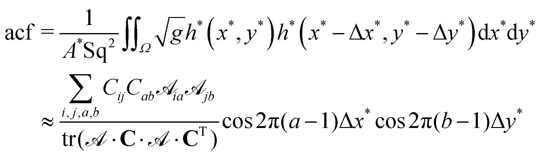 | (21) |
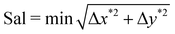 such that acf = c.84 In this manuscript, we adopt c = 0 for achieving uncorrelated conditions.
3 Results
3.1 Direct numerical simulations
Numerical simulations of the nonlinear shape eqn (7) were performed with periodic boundary conditions. We use a pseudo-transient approach to solve this nonlinear PDE by introducing an additional time dimension t* and let t* → +∞.155,156 Once the surface profile converges, the average value cm is calculated numerically as imposed by the vanishing mean condition. The dimensionless relative error for this iterative approach is defined as error = 100% × ‖h*,j+1 − h*,j‖/‖h*,j‖, where h*,j represents h* at the jth time step. We adapt a finite difference approach on the space and an explicit Euler approach on the time dimension. Due to the regularity of the heat operator ∂t* − ∇*2 and the periodic boundary condition, the initial condition can be chosen randomly. The Courant–Friedrichs–Lewy condition is modified specifically for this nonlinear PDE by Δt* = (α/4)·(Δx*)2, where α = 0.1 for a fast and stable calculation. Fig. 4 shows the numerical solution of a surface wrinkling under ε2 = −0.1, ε4 = +0.08 and ε6 = −0.06. | ||
| Fig. 4 Numerical simulations performed on a 51 × 51-grid, with dimensionless anchoring parameters ε2 = −0.1, ε4 = +0.08 and ε6 = −0.06. The iteration terminates if the dimensionless relative error reaches δ = 10−6. (a) Initial condition hinitial = 10−5|ε2/π|rand(0,1); (b) initial condition hinitial = |ε2/π|rand(0,1); (c) and (d) are the iteration-error plot when the simulation starts at initial condition (a) and (b), respectively; (e) the converged numerical solution; (f) the linear approximation. | ||
To confirm that the algorithm is irrelevant to the distribution and magnitude of the initial guess, we adopt a random field multiplied by a magnitude factor. Fig. 4(a) adopts a much smaller initial guess ∼10−5|ε2/π| while Fig. 4(b) uses an initial guess ∼|ε2/π|. The simulations with different initial guesses converge to the same solution (Fig. 4(e)). Fig. 4(c) and (d) are the iteration-error plots for Fig. 4(a) and (b), respectively. Comparing Fig. 4(c) and (d), we see that if the initial guess is very far from the real solution, the iterative method is overly slow (∼106 steps to converge) and the initial error becomes much larger (∼102). Fig. 4(f) is the analytic solution obtained from eqn (11). Comparing Fig. 4(e) and (f), we conclude that the analytic approximation gives a very precise approximation to the numerical solution.
3.2 Surface roughness
In this section, we study the surface roughness of the wrinkling profile discussed in Section 3.1 (see representative result of Fig. 4(e)). Table 2 summarizes all surface roughness parameters studied in this section. . The curve of minima follows a straight line (black line) given by r2 = −0.7793r1 − 0.338. The global minimum
  is found when r1 = −1.43 and r2 = 0.78.
 | ||
Fig. 5 The analytic result of the average magnitude of mean curvature  defined in eqn (14). The minimum curve follows a straight line r2 = −0.7793r1 − 0.3380. The global minimum (white point) is achieved when r1 = −1.43 and r2 = 0.78, with corresponding value defined in eqn (14). The minimum curve follows a straight line r2 = −0.7793r1 − 0.3380. The global minimum (white point) is achieved when r1 = −1.43 and r2 = 0.78, with corresponding value  . . | ||
Fig. 5 shows that the wrinkling profile without higher-order harmonics (r1 = r2 = 0) does not show a minimized average curvature  . Following a linear relation r2 = −0.7793r1 − 0.338 and introducing higher-order harmonics reduces the average magnitude of curvature. Since the linear relation is a straight line that does not pass the first quadrant, the minimum cannot be reached when the anchoring coefficients ε2, ε4, and ε6 are of the same sign. The global minimum (r1 = −1.43, r2 = +0.78) reveals that to obtain a small average magnitude of curvature, the anchoring coefficients should alternate their signs such that sgn(ε2, ε4, ε6) = (+, −, +) or (−, +, −).
These important observations can be verified from the linear approximation. Minimizing  with respect to either r1 or r2 requires linear calculations of Cab(∂Cij/∂r), which is a linear function of r1 and r2. Therefore, the linear approximation confirms that there exists a linear function that minimizes the average magnitude of mean curvature. The linear approximation also verifies that
 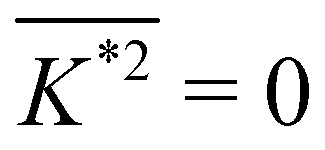 , where details are given in the ESI.† For clarity, we refer to surface with a minimum
  as the
  surface. Table 3 summarizes the numerical results and the linear approximation for the
  surface, and Fig. 6 shows the direct numerical simulations for
  surface.
| Surface parameter | Analytic result | Numerical result |
|---|---|---|

|
0.0643 | 0.0567 |
|
0.0643 | 0.0566 |

|
0 | 5.5 × 10⁻⁵ |

|
0.1286 | 0.1133 |
| Rsk | 0.3217 | 0.2265 |
| Rku | 2.1024 | 2.1124 |
 | ||
Fig. 6 Numerical simulation for surface with ε2 = −0.1, r1 = −1.43, and r2 = 0.78. (a) Is the analytic approximation of the surface. (b) Is the numerical simulation performed on a 251 × 251-grid with tolerance δ = 10−6. (c) Is the (x*, y*) heat map of (b). (d)–(h) Are the dimensionless curvature heat map plots of the numerical surface profile. (d)–(h) Are the dimensionless mean curvature H*, dimensionless Gaussian curvature K*, dimensionless deviatoric curvature D*, dimensionless Casorati curvature C* and the dimensionless shape parameter S, respectively. The calculated average curvatures are  , , 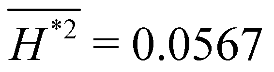 , ,  , and , and 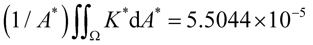 . These values are summarized in Table 3. . These values are summarized in Table 3. | ||
Fig. 6(a) and (b) show the analytic solution and the direct numerical simulation of the  surface, respectively. Fig. 6(c) shows the top view of the numerical solution. The dimensionless (scaled by P0) mean curvature H*, Gaussian curvature K*, deviatoric curvature D*, Casorati curvature C* and normalized shape parameter S of the
  surface are shown in Fig. 6(d)–(h), respectively. Comparing Fig. 6 and 4, we conclude that the
  surface demonstrates few surface kinks near the boundary. Intuitively, the emergence of kinks introduces extra surface patches with low magnitude of curvature. This intuition matches Fig. 6(d), where green semi-rings (H*2 = 0) appear around those kinks. This intuition is also confirmed by the dark blue semi-rings (D*2 = 0) in Fig. 6(f). The
  surface demonstrates complex curvature profiles shown in Fig. 6, with topological constraint that surface integral of those curvatures must satisfy
 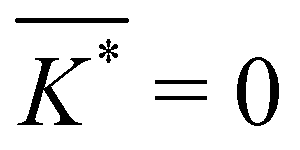 , and
, and  . In addition, if we compare Fig. 6(d) and (e) with (g) and (h) we see that separating curvedness (C*) from shape (S) show directly where we have saddles (S = 0), cylinder (S = ±1/2), and spheres (S = ±1), and what is the curvedness at the geometric transitions between these shapes. Fig. 6 demonstrates that the higher-order anchoring model together with a doubly-periodic director field is a generator of periodic surface patterns with a rich distribution of saddles, cups/domes, and saddles with a distribution of large and small curvedness patches as required in highly functional topographies.
In partial summary,  is a good indicator to describe the surface roughness by evaluating the curvature distribution of each point. The linear approach given in eqn (11) is not only a good approximation of the surface profile h*, but also a good approximation of its second derivative (validated in Table 3). The advantage of
  -method is that
 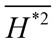 has physical significance (such as the Willmore energy or the Helfrich energy), and the disadvantage is that the surface equation must be at least twice differentiable. Lastly, with a representative result of surface roughness in a CLC given in Fig. 6, we demonstrate that the generalized higher-order liquid crystal shape equation has the potential to generate complex roughness, with distributed saddles, cups/domes, and cylindrical shapes, which can be fine-tuned by anchoring coefficients and surface director orientation. This parametric tuning is performed in detail through roughness calculations of biological surfaces and summarized in Table 4 later in Section 3.3.
| Surface | (Rsk, Rku) | (r1, r2) if ε2 < 0 | (ΔRsk, ΔRku) if ε2 < 0 | (r1, r2) if ε2 > 0 | (ΔRsk, ΔRku) if ε2 > 0 |
|---|---|---|---|---|---|
| Trout with mucus (Salmo trutta) | (0.15, 3.3) | (−3.4068, 2.6338) | (−3.4 × 10⁻³, −4 × 10⁻⁴) | (0.5386, −2.0672) | (−2.79 × 10⁻⁴, −4.1 × 10⁻⁵) |
| Red maple leaf (Acer rubrum) | (0.42, 4.3) | (−3.4420, 2.7033) | (7.01 × 10⁻⁴, 2.56 × 10⁻⁴) | (0.7490, −2.4101) | (6.5 × 10⁻⁵, 2.5 × 10⁻⁵) |
| Back of hand (Homo sapiens) | (−0.19, 3.5) | (0.8355, −2.4307) | (−1.45 × 10⁻⁴, −2.5 × 10⁻⁵) | (−3.4273, 2.6624) | (−4.86 × 10⁻⁴, −5.6 × 10⁻⁵) |
| Flying lizard (Draco timorensis) | (0.56, 3.2) | (−2.2553, 1.6458) | (−2.4 × 10⁻⁵, 5 × 10⁻⁶) | (−2.7490, 1.6366) | (1.63 × 10⁻⁴, 6.2 × 10⁻⁵) |
 | ||
Fig. 7 The analytic result of surface roughness in the (r1, r2) parametric space. (a)–(d) Are the scaled (πSq/ε2)2 plot, the skewness plot and the kurtosis plot for (r1, r2) ∈ [−5, +5]2, respectively. (c) Shows the second quadrant of (b). (e) and (f) Show the second and the fourth quadrants of (d), respectively. The global minima for (πSq/ε2)2 > 0 and Rku > 0 are marked with white dots. The  surface is marked with a magenta dot. The location and the minimized values are: (a) r1 = −2.92, r2 = +2.08 and min{(πSq/ε2)2} = 3.8742 × 10⁻⁴. (d) r1 = −2.86, r2 = +1.98 and min{Rku} = 1.8833. surface is marked with a magenta dot. The location and the minimized values are: (a) r1 = −2.92, r2 = +2.08 and min{(πSq/ε2)2} = 3.8742 × 10⁻⁴. (d) r1 = −2.86, r2 = +1.98 and min{Rku} = 1.8833. | ||
In Fig. 7(a). (πSq/ε2)2 ≥ 0 demonstrates a global minimum (white point) of 3.8742 × 10⁻⁴ at r1 = −2.92 and r2 = +2.08. The global minimum emerges due to the nature of a second-order polynomial  in eqn (17). The surface kurtosis is a polynomial of the form
  from eqn (19). The complexity of the polynomial demonstrates an entangled Rku(r1, r2)-plot, shown in Fig. 7(d)–(f). Rku(r1, r2) is strictly non-negative and it demonstrates a global minimum. The global minimum of Rku is marked with a white point in Fig. 7(d). The global minimum min(Rku) = 1.8833 is reached when r1 = −2.86 and r2 = +1.98. Fig. 7(e) and (f) are the second and fourth quadrants of Fig. 7(d). In Fig. 7(d), we conclude that Rku changes rapidly near the global minimum.
The skewness is a polynomial of the form  , and the density map is shown in Fig. 7(b) and (c). We mark the two global minimum points that minimize Sq and Rku as white dots, and mark the point that minimizes
  (from Fig. 5) as a magenta dot in Fig. 7(b) and (c). The two global minimum points, minSq2 and min{Rku} are located very close to each other, while
  lays further. In Fig. 7(c), the green-cyan colour represents a skewness-free surface. The green-cyan boundaries start to diverge at the minSq2 and min{Rku} points. And the global minimum point
  is located inside a green-cyan region, showing a small Rsk value. The numerical value and analytic result are given in Table 3.
According to the definition, the skewness and kurtosis are scaled by the root mean square and are dimensionless, which results a scale-independent Rsk–Rku plot shown in Fig. 8. The Rsk–Rku plot is widely used in surface manufacturing.157,158 For example, Rsk ranges from −1 to + 1 for most surface machining process.159Fig. 8 shows a wide range of Rsk and Rku. There are two bounds in Fig. 8. The first bound Rku ≥ Rsk2 + 1 is an inequality resulting from the definition (derivation is given in the ESI,† where equality holds strictly for Bernoulli distributions152,158,160). The second bound Rku ≥ 1.8833 is physical, which implies that it is impossible to obtain an anchoring-driven CLC surface with a lower Rku. The Rapini–Papoular anchoring model cannot generate a surface with low Rsk and high Rku. The intersections between the curves imply that an inverse problem does not have a unique solution, i.e., different combination of r1 and r2 can generate a surface with the same Rku and Rsk. Other surface roughness parameters are required to determine the anchoring coefficients. The inverse problem will be discussed in Section 3.3.
 | ||
| Fig. 8 The surface skewness and kurtosis plot. The curves are taken when r1 = −5, −4.5,…, + 5. The region below the curve Rku = Rsk2 + 1 is a mathematically impossible zone, and the region below Rku < 1.8833 is a physically impossible zone. | ||
In partial summary, the method of higher-order moments evaluates the variance, bias and peakness of surface wrinkling. It shows that the Rapini-Rapoular model contains intrinsic bounds of root mean square and kurtosis. We also concluded that different anchoring coefficient ratios may result the same surface roughness parameters. To distinguish different surfaces with same Rsk and Rku, other methods should be incorporated. For example, introducing the 5th and 6th-order moment for calculating hyperskewness and hypertailedness.
Fig. 9(a)–(c) show the autocorrelation function acf as a function of lagging (Δx*, Δy*) for the min{(πSqε2)2} surface, the min{Rku} surface, and the  surface. The white curves denote the region where acf function vanishes. The autocorrelation length Sal is the radius of the circle tangent to the closest white curve. Fig. 9(d) demonstrates the three regions of the C-matrix: the low-frequency block, the mid-frequency block and the high-frequency block. Comparing Fig. 9(b) and (c), the autocorrelation length for min{Rku} is Sal = 0.0703 which is smaller than that of the
  surface (Sal = 0.1691). Fig. 9(e) and (f) are the C-matrix visualization (scaled by
  ) of (b) and (c), where (c) is a low-frequency dominated profile (64.1%). Fig. 9 demonstrates that Sal is the proper surface roughness parameter that recognizes the frequency of the surface profile without considering the magnitude of the wrinkling.
 | ||
Fig. 9 Normalized autocorrelation function of (a) min{(πSq/ε2)2} point, r1 = −2.92 and r2 = +2.08. Sal = 0.0692 when (Δx*, Δy*) = (0.042, 0.055); (b) min{Rku} point, r1 = −2.86 and r2 = +1.98. Sal = 0.0703 when (Δx*, Δy*) = (0.045, 0.054); (c)  point, r1 = −1.43 and r2 = +0.78. Sal = 0.1691 when (Δx*, Δy*) = (0.131, 0.107). From (a) to (c), white curves represent acf = 0. (d) C-Matrix can be split into three zones: low-frequency region, mid-frequency region, and high-frequency region. (e) The contribution heat map of the absolute value of each element in C-matrix for min{Rku} point (corresponding to (b)). The contribution ratio of each region is low:mid:high = 9.4:40.3:50.3. (f) The same C-matrix visualization for min{ point, r1 = −1.43 and r2 = +0.78. Sal = 0.1691 when (Δx*, Δy*) = (0.131, 0.107). From (a) to (c), white curves represent acf = 0. (d) C-Matrix can be split into three zones: low-frequency region, mid-frequency region, and high-frequency region. (e) The contribution heat map of the absolute value of each element in C-matrix for min{Rku} point (corresponding to (b)). The contribution ratio of each region is low:mid:high = 9.4:40.3:50.3. (f) The same C-matrix visualization for min{![[C with combining macron]](https://www.rsc.org/images/entities/i_char_0043_0304.gif) *2} point (corresponding to (c)). The contribution ratio of each region is low:mid:high = 64.1:24.0:11.9. Comparing (e) and (f), we can observe that low frequency dominated profile (64.1%) shows a high Sal, while high frequency dominated profile (50.3%) shows a lower Sal. *2} point (corresponding to (c)). The contribution ratio of each region is low:mid:high = 64.1:24.0:11.9. Comparing (e) and (f), we can observe that low frequency dominated profile (64.1%) shows a high Sal, while high frequency dominated profile (50.3%) shows a lower Sal. | ||
In partial summary, autocorrelation function and autocorrelation length evaluate the correlation between the surface with its lagged copy. They are dependent to the (x*, y*)-direction and irrelevant to the h*-direction. Noteworthy, larger Sal implies a surface that is dominated by low spatial frequency asperities, which agrees with the literature.161
3.3 Application and inverse problem
The skewness and kurtosis of a sample's surface profile are easier to measure compared to the anchoring coefficients. By solving the nonlinear eqn (18) and (19), this paper provides an alternative way to measure the anchoring coefficients. However, there are two concerns appearing in this approach. The first concern is that functions (18) and (19) are surjective-only, which are verified by Fig. 8. The intersections in Fig. 8 demonstrate that there is no unique pair of r1 and r2 that yield the given values of skewness and kurtosis. The second concern is that eqn (18) contains the sign of ε2, and the final solutions are anchoring ratio vector , which is irrelevant to ε2. To address the problem, we implement an optimization approach to find the anchoring coefficients that are closest to zero since the magnitude of those coefficients tend to be very small (|ε2i| ≪ 1). We can solve this inverse problem
  via a Levenberg–Marquardt algorithm with an updating formula
 | (22) |
 | (23) |
The surface skewness and kurtosis data are obtained in literature.162 And two possible (r1, r2) pairs are given for positive and negative ε2. The deviation of each case is very low. The error-iteration plot and the determinant of Jacobian matrix for the surface of Salmo trutta are shown in Fig. 10. By reducing the penalty parameter λ, the calculation converges faster. However, if λ is very small (λ < 10−4), the calculation diverges because the Jacobian becomes singular. Fig. 10(b) shows that increasing penalty parameter can also cause a singular Jacobian.
 | ||
| Fig. 10 (a) Convergence plot of the surface Salmo trutta by using different penalty factor λ. (b) Salmo trutta cannot be solved directly from Newton–Raphson method due to the singular Jacobian matrix. Large λ (such as λ > 0.5), small λ (such as λ < 0.0001) or inappropriate choice (such as λ = 0.9) lead to divergence. | ||
In partial summary, we show that the inverse problem is an ill-posed problem, and we cannot guarantee a unique, stable result without introducing more information. Some of the alternatives are: (1) find the anchoring coefficients that are closest to zero; (2) compute higher-order (more than 4th-order) moment of the surface profile and conclude the unique anchoring coefficients. This method is also equivalent to method of moments in classical statistical inference.163
4. Conclusions
In summary, we studied the wrinkling profiles of biological and synthetic cholesteric liquid crystals driven by surface anchoring, using a generalized Rapini–Papoular model of order 2m. We obtained the analytic solution of the surface wrinkling model under a small-wrinkling approximation, where the surface profile is a linear combination of 4m(m + 1) distinct wrinkling modes. The direct numerical simulation validates our linearized solutions. We conducted a comprehensive examination of the surface roughness by adapting statistical approaches from hard surfaces, and we developed a curvature-based method of soft surfaces. In this paper, the surface roughness of CLC surfaces driven by anchoring is studied through evaluating the curvature, higher-order moments, autocorrelation function and autocorrelation length. The numerical simulation predicts that the average magnitude of the scaled mean curvature has a lower bound of 0.0643, achieved when the signs of three anchoring coefficients (μ2, μ4, μ6) alternate. We studied the 2nd to the 4th-order moments of the surface profile, which correspond to the root mean square (Sq), skewness (Rsk), and kurtosis (Rku). The root mean square characterizes the surface deviation, and the skewness and kurtosis evaluates the bias and sharpness/peakness. We also concluded the lower bounds of both Sq and Rku in the Rapini–Papoular model. The lower bounds are achieved when the anchoring coefficients alternate sign. The autocorrelation function (acf) and autocorrelation length (Sal) distinguish a low- or a high-frequency dominated surface, and they provide a visualization of the 4m(m + 1) distinct wrinkling modes.Finally, we studied the inverse engineering problem. The inverse engineering problem aims to find the indirect anchoring coefficients (material property) by measuring the direct surface roughness. The significance of the inverse problem is that it reverses the difficulty of experiments, since the surface profile (the result of forward problem) is generally easier to obtain than the physics (input of the forward problem). However, the inverse problem is ill-posed, and it requires more information to provide unique and stable anchoring coefficients. Restricted by the lack of experimental data in literature, we calculated the anchoring coefficients of some biological systems by assuming they are close to zero. Our approach can be generalized to calculate r3, r4, …, etc. if the data of higher-order moments are available.
The significance and original contributions are summarized as follow:
1. Surface wrinkling profile is a linear combination of different fundamental wrinkling modes. The C-matrix provides details of frequency analysis and the autocorrelation function/length demonstrates a method of visualization: Fig. 2 and 9, eqn (21).
2. We provide the analytic solution for surface wrinkling under small-wrinkling approximation. The analytic solution matches with numerical solution. The curvature distribution shows rich complexity needed for multifunctionality: Fig. 4 and 6, eqn (11).
3. A curvature-based approach  is shown to be an proper surface roughness parameter, which also serves to quantify definitions of surface energy: Fig. 5, eqn (16).
4. Higher-order statistical moments are widely used in studying metal surface roughness, and they are shown to be suitable for soft matter surfaces in this paper: Fig. 7 and 8, eqn (17)–(19), Tables 2 and 3.
5. The inverse engineering problem provides a promising application that measures surface anchoring coefficients based on simple experiment: Fig. 10, eqn (22).
In conclusion, this paper combines theoretical and numerical insights into the study of biological and synthetic cholesteric liquid crystals surfaces. With a comprehensive understanding of the surface wrinkling profiles induced by anchoring, the theoretical framework, numerical simulations, and conclusions presented in this paper have potential applications in roughness-dominated processes and phenomena in both industry and biology.
Author contributions
ZW wrote the original draft. PS and ADR reviewed and edited the manuscript. ZW contributed to the data curation and visualization. PS and ADR contributed to the funding acquisition, supervision and project administration. ZW, PS and ADR contributed to the conceptualization, formal analysis and methodology.Data availability
The data and derivations supporting this article have been included as part of the ESI.† The scheme implemented in this research is a standard finite difference approach. The software and data visualization tool used in this research is MatLab.Conflicts of interest
There are no conflicts to declare.Acknowledgements
This work was supported by the Natural Science and Engineering Research Council of Canada (NSERC) (Grant number: 223086). AR thanks McGill University for financial support through the James McGill Professor appointment. This research was enabled in part by the support provided by Calcul Québec, the BC DRI Group, and the Digital Research Alliance of Canada (https://alliancecan.ca/alliancecan.ca). ZW thanks the Faculty of Engineering for the MEDA scholarship program to assist his PhD study.Notes and references
- M. Roth, M. D’Acunzi, D. Vollmer and G. K. Auernhammer, J. Chem. Phys., 2010, 132, 124702 CrossRef CAS PubMed.
- A. D. Rey, Rheol. Acta, 1996, 35, 400–409 CrossRef CAS.
- F. Giavazzi, S. Crotti, A. Speciale, F. Serra, G. Zanchetta, V. Trappe, M. Buscaglia, T. Bellini and R. Cerbino, Soft Matter, 2014, 10, 3938–3949 RSC.
- H. K. Bisoyi and Q. Li, Acc. Chem. Res., 2014, 47, 3184–3195 CrossRef CAS PubMed.
- Z.-g Zheng, Y. Li, H. K. Bisoyi, L. Wang, T. J. Bunning and Q. Li, Nature, 2016, 531, 352–356 CrossRef CAS PubMed.
- I. Dierking, Symmetry, 2014, 6, 444–472 CrossRef.
- V. Sharma, M. Crne, J. O. Park and M. Srinivasarao, Mater. Today: Proc., 2014, 1, 161–171 Search PubMed.
- Y. Tang, C. Lu and R. Xiong, ACS Nano, 2024, 18, 14629–14639 CrossRef CAS.
- Y. Luo, Y. Li, K. Liu, L. Li, W. Wen, S. Ding, Y. Huang, M. Liu, C. Zhou and B. Luo, Biomacromolecules, 2023, 24, 2942–2954 CrossRef CAS PubMed.
- Y. Bouligand, Tissue Cell, 1972, 4, 189–217 CrossRef CAS.
- Y. Bouligand, C. R. Chim, 2008, 11, 281–296 CrossRef CAS.
- K. M. Lee, V. P. Tondiglia, M. Rumi and T. J. White, J. Polym. Sci., Part B: Polym. Phys., 2018, 56, 1087–1093 CrossRef CAS.
- J.-S. Hu, B.-Y. Zhang, Y.-Y. Zheng and Q.-Y. Li, React. Funct. Polym., 2005, 64, 1–11 CrossRef CAS.
- B.-Y. Zhang, J.-S. Hu, Y.-G. Jia and B.-G. Du, Macromol. Chem. Phys., 2003, 204, 2123–2129 CrossRef CAS.
- F. Kameche, W. Heni, S. Telitel, D. Ge, L. Vidal, F. Dumur, D. Gigmes, J. Lalevee, S. Marguet and L. Douillard, et al. , Mater. Today, 2020, 40, 38–47 CrossRef CAS.
- Y. Wang, S. Wang, S. Zhang, O. A. Scherman, J. J. Baumberg, T. Ding and H. Xu, Nano Res., 2018, 11, 6384–6390 CrossRef CAS.
- Z. Liang, Y. Zhao, H. Gao, D. Wang, Z. Miao, H. Cao, Z. Yang and W. He, Liq. Cryst., 2021, 48, 2016–2026 CrossRef CAS.
- J. Liu, S. Zhang, Z. Wang, X. Xia, J. Zhang, Y. Yu, Y. Xiao, Y. Ren, J. Chen and B. Yang, et al. , Nat. Commun., 2024, 15, 1–11 Search PubMed.
- M. Mitov, Soft Matter, 2017, 13, 4176–4209 RSC.
- A. Scarangella, V. Soldan and M. Mitov, Nat. Commun., 2020, 11, 4108 CrossRef CAS.
- O. F. A. Gutierrez and A. D. Rey, Soft Matter, 2017, 13, 8076–8088 RSC.
- P. Rofouie, D. Pasini and A. D. Rey, Colloid Interface Sci. Commun., 2014, 1, 23–26 CrossRef CAS.
- M.-M. Giraud-Guille, L. Besseau and R. Martin, J. Biomech., 2003, 36, 1571–1579 CrossRef.
- M. M. G. Guille, G. Mosser, C. Helary and D. Eglin, Micron, 2005, 36, 602–608 CrossRef.
- M. H. Chow, K. T. Yan, M. J. Bennett and J. T. Wong, Eukaryotic Cell, 2010, 9, 1577–1587 CrossRef CAS.
- S. L. Ilca, X. Sun, K. El Omari, A. Kotecha, F. de Haas, F. DiMaio, J. M. Grimes, D. I. Stuart, M. M. Poranen and J. T. Huiskonen, Nature, 2019, 570, 252–256 CrossRef CAS.
- J. A. Kluge, O. Rabotyagova, G. G. Leisk and D. L. Kaplan, Trends Biotechnol., 2008, 26, 244–251 CrossRef CAS PubMed.
- D. Saravanan, et al. , J. Text. Apparel, Technol. Manage., 2006, 5, 1–20 Search PubMed.
- R. Kemkemer, D. Kling, D. Kaufmann and H. Gruler, Eur. Phys. J. E: Soft Matter Biol. Phys., 2000, 1, 215–225 CrossRef CAS.
- R. Kemkemer, V. Teichgräber, S. Schrank-Kaufmann, D. Kaufmann and H. Gruler, Eur. Phys. J. E:Soft Matter Biol. Phys., 2000, 3, 101–110 CrossRef CAS.
- Y. Tan, B. Hu, J. Song, Z. Chu and W. Wu, Nano-Micro Lett., 2020, 12, 1–42 CrossRef PubMed.
- P. J. Yoo and H. H. Lee, Macromolecules, 2005, 38, 2820–2831 CrossRef CAS.
- X.-F. Wu, Y. A. Dzenis and K. W. Strabala, Meccanica, 2007, 42, 273–282 CrossRef.
- A. Cutolo, V. Pagliarulo, F. Merola, S. Coppola, P. Ferraro and M. Fraldi, Mater. Des., 2020, 187, 108314 CrossRef CAS.
- L. Jin, PhD thesis, Harvard University, 2014.
- Q. Wang and X. Zhao, Sci. Rep., 2015, 5, 8887 CrossRef CAS.
- V. Trujillo, J. Kim and R. C. Hayward, Soft Matter, 2008, 4, 564–569 RSC.
- B. Dortdivanlioglu, N. E. D. Yilmaz, K. Goh, X. Zheng and C. Linder, J. Elasticity, 2021, 1–17 Search PubMed.
- W. Hong, X. Zhao and Z. Suo, Appl. Phys. Lett., 2009, 95, 111901 CrossRef.
- D. Chen, S. Cai, Z. Suo and R. C. Hayward, Phys. Rev. Lett., 2012, 109, 038001 CrossRef.
- Q. Liu, T. Ouchi, L. Jin, R. Hayward and Z. Suo, Phys. Rev. Lett., 2019, 122, 098003 CrossRef CAS.
- L. Norlén, J. Invest. Dermatol., 2001, 117, 823–829 CrossRef.
- G. Perkins and T. Frey, Micron, 2000, 31, 97–111 CrossRef CAS.
- F. Joubert and N. Puff, Membranes, 2021, 11, 465 CrossRef CAS PubMed.
- J.-F. Mangin, D. Riviere, A. Cachia, E. Duchesnay, Y. Cointepas, D. Papadopoulos-Orfanos, P. Scifo, T. Ochiai, F. Brunelle and J. Régis, NeuroImage, 2004, 23, S129–S138 CrossRef.
- K. Garcia, C. Kroenke and P. Bayly, Philos. Trans. R. Soc., B, 2018, 373, 20170321 CrossRef.
- G. F. Striedter, S. Srinivasan and E. S. Monuki, Annu. Rev. Neurosci., 2015, 38, 291–307 CrossRef CAS PubMed.
- F. H. P. de Moraes, F. Sudo, M. Carneiro Monteiro, B. R. de Melo, P. Mattos, B. Mota and F. Tovar-Moll, Sci. Rep., 2024, 14, 3222 CrossRef CAS.
- P. Rofouie, D. Pasini and A. D. Rey, Soft Matter, 2015, 11, 1127–1139 RSC.
- P. Rofouie, D. Pasini and A. D. Rey, Soft Matter, 2017, 13, 5366–5380 RSC.
- H. Goto, IOP Conference Series: Materials Science and Engineering, 2014, p. 012013 Search PubMed.
- H. Nagai, X. Liang, Y. Nishikawa, K. Nakajima and K. Urayama, Macromolecules, 2016, 49, 9561–9567 CrossRef CAS.
- Z. Wang, P. Servio and A. Rey, Colloid Interface Sci. Commun., 2021, 41, 100372 CrossRef CAS.
- Z. Wang, P. Servio and A. D. Rey, Nanomaterials, 2022, 12, 1555 CrossRef CAS.
- Z. Wang, P. Servio and A. Rey, Phys. Rev. E, 2022, 105, 034702 CrossRef CAS.
- A. Ryabchun and A. Bobrovsky, Adv. Opt. Mater., 2018, 6, 1800335 CrossRef.
- I. Tobasco, Y. Timounay, D. Todorova, G. C. Leggat, J. D. Paulsen and E. Katifori, Nat. Phys., 2022, 18, 1099–1104 Search PubMed.
- T. Wen, T. Ma, J. Qian, Z. Song, X. Jiang and Y. Yao, Nat. Commun., 2024, 15, 10821 Search PubMed.
- Z. Wang, P. Rofouie and A. D. Rey, Crystals, 2019, 9, 190 Search PubMed.
- Z. Wang, P. Servio and A. D. Rey, Phys. Rev. E, 2020, 101, 062705 CrossRef CAS.
- Z. Wang, P. Servio and A. D. Rey, Front. Soft Matter, 2022, 2, 904069 CrossRef.
- Z. Wang, P. Servio and A. D. Rey, Soft Matter, 2023, 19, 9344 RSC.
- Z. Wang, P. Servio and A. D. Rey, Front. Soft Matter, 2023, 3, 1123324 CrossRef.
- A.-G. Cheong, A. D. Rey and P. T. Mather, Phys. Rev. E: Stat., Nonlinear, Soft Matter Phys., 2001, 64, 041701 CrossRef CAS.
- A.-G. Cheong and A. D. Rey, J. Chem. Phys., 2002, 117, 5062–5071 CrossRef CAS.
- A.-G. Cheong and A. D. Rey, Phys. Rev. E: Stat., Nonlinear, Soft Matter Phys., 2002, 66, 021704 CrossRef.
- A.-G. Cheong and A. D. Rey, Continuum Mech. Thermodyn., 2002, 14, 263–279 CrossRef CAS.
- A.-G. Cheong and A. D. Rey, Liq. Cryst., 2004, 31, 1271–1284 CrossRef CAS.
- S. Schauer, M. Worgull and H. Hölscher, Soft Matter, 2017, 13, 4328–4334 RSC.
- Y. Nakamura and Y. Tomonari, J. Fluid Mech., 1982, 123, 363–378 CrossRef CAS.
- F. Farshad, H. Rieke and J. Garber, J. Pet. Sci. Eng., 2001, 29, 139–150 CrossRef CAS.
- G. Severino, J. Fluid Mech., 2024, 1000, R1 CrossRef CAS.
- W.-K. Hong, S. Song, D.-K. Hwang, S.-S. Kwon, G. Jo, S.-J. Park and T. Lee, Appl. Surf. Sci., 2008, 254, 7559–7564 CrossRef CAS.
- G. Palasantzas, J. T. M. De Hosson and J. Barnas, Surf. Sci., 2002, 507, 541–545 CrossRef.
- A. Larena, F. Millán, G. Pérez and G. Pinto, Appl. Surf. Sci., 2002, 187, 339–346 CrossRef CAS.
- A. Trügler, J.-C. Tinguely, J. R. Krenn, A. Hohenau and U. Hohenester, Phys. Rev. B: Condens. Matter Mater. Phys., 2011, 83, 081412 CrossRef.
- K. Kubiak, M. Wilson, T. Mathia and P. Carval, Wear, 2011, 271, 523–528 CrossRef CAS.
- A. AlRatrout, M. J. Blunt and B. Bijeljic, Proc. Natl. Acad. Sci. U. S. A., 2018, 115, 8901–8906 CrossRef CAS.
- B. N. Persson, O. Albohr, U. Tartaglino, A. I. Volokitin and E. Tosatti, J. Phys.: Condens. Matter, 2004, 17, R1 CrossRef.
- F. Svahn, Å. Kassman-Rudolphi and E. Wallén, Wear, 2003, 254, 1092–1098 CrossRef CAS.
- J. Koo and C. Kleinstreuer, Int. J. Heat Mass Transfer, 2005, 48, 2625–2634 CrossRef.
- A. Toloei, V. Stoilov and D. Northwood, ASME International mechanical engineering congress and exposition, 2013, p. V02BT02A054 Search PubMed.
- C. Hagen, A. Hognestad, O. Ø. Knudsen and K. Sørby, Prog. Org. Coat., 2019, 130, 17–23 CrossRef CAS.
- K. Singh, N. Paliwal and K. Kasamias, Sci. Rep., 2024, 14, 1785 CrossRef CAS.
- A. Gujrati, S. R. Khanal, L. Pastewka and T. D. Jacobs, ACS Appl. Mater. Interfaces, 2018, 10, 29169–29178 CrossRef CAS.
- I. J. Cartwright and J. A. Higgins, J. Biol. Chem., 2001, 276, 48048–48057 CrossRef CAS PubMed.
- S. R. Wilkinson, M. C. Taylor, S. Touitha, I. L. Mauricio, D. J. Meyer and J. M. Kelly, Biochem. J., 2002, 364, 787–794 CrossRef CAS PubMed.
- H. F. Lodish, N. Kong, M. Snider and G. J. Strous, Nature, 1983, 304, 80–83 CrossRef CAS PubMed.
- E. C. Mandon, S. F. Trueman and R. Gilmore, Cold Spring Harbor Perspect. Biol., 2013, 5, a013342 Search PubMed.
- E. Kuwert and R. Schätzle, J. Differ. Geom., 2001, 57, 409–441 Search PubMed.
- E. Aulisa, A. Gruber and M. Toda, Geom., Integrability Quantization, Papers Lecture Ser., 2024, 29, 1–10 CrossRef.
- M. Toda and B. Athukoralage, AIP Conference Proceedings, 2013, pp. 883–886 Search PubMed.
- O.-Y. Zhong-Can and W. Helfrich, Phys. Rev. A: At., Mol., Opt. Phys., 1989, 39, 5280 CrossRef.
- F. Campelo, C. Arnarez, S. J. Marrink and M. M. Kozlov, Adv. Colloid Interface Sci., 2014, 208, 25–33 CrossRef CAS.
- W. Helfrich, Giant Vesicles, 1999, 51–70 Search PubMed.
- W. Bao and Y. Li, SIAM J. Numerical Anal., 2025, 63, 103–121 CrossRef.
- G. Dziuk, Numer. Math., 2008, 111, 55–80 CrossRef.
- S. R. Brown, Geophys. Res. Lett., 1987, 14, 1095–1098 CrossRef.
- S. R. Nayak, J. Mishra and G. Palai, Image Vision Comput., 2019, 89, 21–34 CrossRef.
- A. Majumdar and B. Bhushan, J. Tribol., 1990, 112, 205–216 CrossRef.
- A. D. Rey, Langmuir, 2001, 17, 1922–1927 CrossRef CAS.
- D. Schlegel, M. Folea, A. Roman and P. Nardin, Rec. Res. Manuf. Eng., 2011, 152–155 Search PubMed.
- A. W. Hashmi, H. S. Mali, A. Meena, M. F. Hashmi and N. D. Bokde, Comput. Model. Eng. Sci., 2023, 135, 917–1005 Search PubMed.
- C. T. Collier, E. Hesse, L. Taylor, Z. Ulanowski, A. Penttilä and T. Nousiainen, J. Quant. Spectrosc. Radiat. Transfer, 2016, 182, 225–239 Search PubMed.
- C. Tay, S. Wang, C. Quan and H. Shang, Opt. Commun., 2003, 218, 1–10 Search PubMed.
- S. Banerjee, R. Yang, C. E. Courchene and T. E. Conners, Ind. Eng. Chem. Res., 2009, 48, 4322–4325 CrossRef CAS.
- S. Lawes, S. Hainsworth, P. Blake, K. Ryder and A. Abbott, Tribol. Lett., 2010, 37, 103–110 CrossRef CAS.
- S. Al-Jeshi and A. Neville, Desalination, 2006, 189, 221–228 CrossRef CAS.
- N. Almqvist, Surf. Sci., 1996, 355, 221–228 Search PubMed.
- C.-L. Tien, H.-M. Yang and M.-C. Liu, Thin Solid Films, 2009, 517, 5110–5115 CrossRef CAS.
- V. Niola, G. Nasti and G. Quaremba, J. Mater. Process. Technol., 2005, 164, 1410–1415 Search PubMed.
- U. Kühnau, A. Petrov, G. Klose and H. Schmiedel, Phys. Rev. E: Stat. Phys., Plasmas, Fluids, Relat. Interdiscip. Top., 1999, 59, 578 Search PubMed.
- D.-F. Gu, S. Uran and C. Rosenblatt, Liq. Cryst., 1995, 19, 427–431 CrossRef CAS.
- Y. Choi, H. Yokoyama and J. S. Gwag, Opt. Express, 2013, 21, 12135–12144 CrossRef PubMed.
- A. Marino, V. Tkachenko, E. Santamato, N. Bennis, X. Quintana, J. Otón and G. Abbate, J. Appl. Phys., 2010, 107, 073109 CrossRef.
- A. D. Rey, Mol. Cryst. Liq. Cryst. Sci. Technol., Sect. A, 2001, 369, 63–74 CrossRef CAS.
- A. D. Rey, Macromol. Theory Simul., 2004, 13, 686–696 CrossRef CAS.
- A. D. Rey, Soft Matter, 2007, 3, 1349–1368 RSC.
- A. D. Rey, J. Chem. Phys., 2004, 120, 2010–2019 CrossRef CAS.
- A. D. Rey, Rheol. Acta, 2000, 39, 13–19 CrossRef CAS.
- A. D. Rey, Phys. Rev. E: Stat. Phys., Plasmas, Fluids, Relat. Interdiscip. Top., 2000, 61, 1540 CrossRef CAS PubMed.
- A. D. Rey, Macromol. Theory Simul., 2000, 9, 156–165 CrossRef CAS.
- A. D. Rey, E. Herrera-Valencia and Y. K. Murugesan, Liq. Cryst., 2014, 41, 430–451 CrossRef CAS.
- Y. K. Murugesan and A. D. Rey, J. Non-Newtonian Fluid Mech., 2010, 165, 32–44 CrossRef CAS.
- A. D. Rey, J. Non-Newtonian Fluid Mech., 2001, 96, 45–62 Search PubMed.
- D. V. Shmeliova, S. V. Pasechnik, S. S. Kharlamov, A. V. Zakharov, E. P. Pozhidaev, V. A. Barbashov and T. P. Tkachenko, Crystals, 2020, 10, 1029 CrossRef CAS.
- D. V. Shmeliova, S. V. Pasechnik, S. S. Kharlamov, A. V. Dubtsov, A. V. Zakharov, S. Loebner and S. Santer, Symmetry, 2023, 15, 722 CrossRef CAS.
- A. V. Zakharov, Phys. Solid State, 2018, 60, 610–615 CrossRef CAS.
- J. Zhao, X. Yang, Y. Gong and Q. Wang, Comput. Methods Appl. Mech. Eng., 2017, 318, 803–825 CrossRef.
- R. J. Fox, W.-R. Chen, C. Do, S. J. Picken, M. G. Forest and T. J. Dingemans, Rheol. Acta, 2020, 59, 727–743 CrossRef CAS.
- M. G. Forest, Q. Wang and R. Zhou, Soft Matter, 2013, 9, 5207–5222 RSC.
- D. Chillingworth, M. G. Forest, R. Lauterbach and C. Wulff, Arch. Ration. Mech. Anal., 2021, 242, 1229–1287 CrossRef.
- A. D. Rey, J. Chem. Phys., 1999, 110, 9769–9770 CrossRef CAS.
- A. D. Rey, Liq. Cryst., 1999, 26, 913–917 CrossRef CAS.
- A. D. Rey, Phys. Rev. E: Stat. Phys., Plasmas, Fluids, Relat. Interdiscip. Top., 1999, 60, 1077 CrossRef CAS.
- P. Yue, J. J. Feng, C. Liu and J. Shen, J. Colloid Interface Sci., 2005, 290, 281–288 CrossRef CAS.
- F. H. Lin and C. Liu, J. Partial Differ. Equ., 2001, 14, 289–330 Search PubMed.
- C. Liu and H. Sun, Discrete Continuous Dyn. Syst., 2008, 23, 455–475 Search PubMed.
- C. Liu and N. J. Walkington, SIAM J. Numerical Anal., 2000, 37, 725–741 CrossRef.
- A. D. Rey, Phys. Rev. E: Stat., Nonlinear, Soft Matter Phys., 2005, 72, 011706 CrossRef.
- W. Jiang and Q. Zhao, Phys. D, 2019, 390, 69–83 CrossRef.
- J. Cahn and D. Hoffman, Acta Metall., 1974, 22, 1205–1214 CrossRef CAS.
- D. W. Hoffman and J. W. Cahn, Surf. Sci., 1972, 31, 368–388 CrossRef CAS.
- A.-G. Cheong and A. D. Rey, J. Chem. Phys., 2002, 117, 5062–5071 CrossRef CAS.
- O. F. A. Gutierrez and A. D. Rey, Soft Matter, 2018, 14, 1465–1473 RSC.
- Z. Wang, P. Servio and A. D. Rey, Entropy, 2020, 22, 909 CrossRef.
- D. U. Zamora Cisneros, Z. Wang, N.-M. Dorval Courchesne, M. J. Harrington and A. D. Rey, Front. Soft Matter, 2024, 4, 1359128 CrossRef.
- S. Givli, H. Giang and K. Bhattacharya, SIAM J. Appl. Math., 2012, 72, 489–511 CrossRef CAS.
- A. Agrawal, Biomech. Model. Mechanobiol., 2025, 1–5 Search PubMed.
- Z. Tu and Z. Ou-Yang, J. Phys. A: Math. Gen., 2004, 37, 11407 CrossRef CAS.
- P. Podulka, Coatings, 2022, 13, 74 CrossRef.
- A. Francisco and N. Brunetière, Proc. Inst. Mech. Eng., Part J, 2016, 230, 747–768 CrossRef.
- P. Podulka, W. Macek, B. Zima, G. Lesiuk, R. Branco and G. Królczyk, Measurement, 2023, 222, 113640 CrossRef.
- R. Dusséaux and E. Vannier, Biosyst. Eng., 2022, 220, 87–102 CrossRef.
- C. T. Kelley and D. E. Keyes, SIAM J. Numerical Anal., 1998, 35, 508–523 CrossRef.
- X.-l Luo, Appl. Math. Comput., 2010, 216, 1752–1762 CrossRef.
- D. Hüser, J. Hüser, S. Rief, J. Seewig and P. Thomsen-Schmidt, Meas. Sci. Technol., 2016, 27, 085005 CrossRef.
- A. Busse and T. Jelly, J. Turbulence, 2023, 24, 57–81 CrossRef.
- D. J. Whitehouse, Handbook of surface and nanometrology, Taylor & Francis, 2002 Search PubMed.
- K. Pearson, Philos. Trans. R. Soc., A, 1916, 216, 429–457 Search PubMed.
- S. Panda, A. Panzade, M. Sarangi and S. Roy Chowdhury, J. Tribol., 2017, 139, 031402 CrossRef.
- D. K. Wainwright, G. V. Lauder and J. C. Weaver, Methods Ecol. Evolution, 2017, 8, 1626–1638 Search PubMed.
- L. Wasserman, All of statistics: a concise course in statistical inference, Springer Science & Business Media, 2013 Search PubMed.
Footnote |
| † Electronic supplementary information (ESI) available. See DOI: https://doi.org/10.1039/d5sm00121h |
| This journal is © The Royal Society of Chemistry 2025 |