Microplastics in the rough: using data augmentation to identify plastics contaminated by water and plant matter

Abstract

Microplastics are present in nearly all environments. The detection of microplastics in the field is an important step toward understanding and regulating the proliferation of plastic waste, particularly in natural environments. Real-time surveys require robust instruments, rapid acquisition, and minimal processing. Near infrared (NIR) spectroscopy is an ideal technique to detect polymer composition regardless of spectral interference by water and/or organic matter. Here we report a fiber-based NIR instrument designed for simple and efficient spectral acquisition of consumer plastic particles across a range of sizes. Data augmentation with measured interferent spectra has been used to generate machine-learning based classification models that can identify polymer compositions in plastic particles that are wet and/or mixed in with organic plant material. These models achieve 98.5% accuracy on synthetic data and 86.4% accuracy when transferred to spectra of plastic particles of nine common polymers with particle sizes as small as 500 μm. Our model paves the way for the development of equipment to perform real-time surveys of microplastic compositions in the field.

---

Sustainability spotlight

Microplastics are a growing global environmental concern, contaminating soil and water. Measuring their presence is the first step in mitigating pollution and its effects on ecosystems and human health. This work advances sustainability by providing an efficient, field-deployable method for identifying microplastics even in contaminated environments. By using near-infrared (NIR) spectroscopy coupled with machine learning, the method accurately detects common polymers despite interference from water and plant materials, supporting the reduction and management of plastic waste. This research aligns with UN Sustainable Development Goals: Clean Water and Sanitation as well as Responsible Consumption and Production, promoting environmental protection and sustainable waste management.

1 Introduction

Plastic waste is an increasingly challenging global problem. The OECD has found that plastic waste generation has more than doubled between 2000 and 2019.¹ Sources of plastic include both commercial and consumer products.^2,3 Both macroscale plastic pollution and microplastics cause harm to terrestrial, aerial, and aquatic organisms.^4–7 Larger scale plastics (>1 mm) are often connected with physical damage to organisms, while smaller plastics can accumulate in tissues or interact with metabolic pathways.^8,9 Microplastics, which are less than 5 mm in size, span both regimes. Their presence even in remote regions such as polar ice and marine sediments, further emphasizes their global prevalence and persistence in the environment.^10,11 These small plastics can be directly introduced into the environment or be the result of cracking or degradation of larger objects.¹² One specific issue with microplastics, due to their small size, is that they can be carried and distributed throughout the environment by a variety of factors including waterways, tides, and wind.^8,13,14 Due to the numerous sources and methods of dispersion, detailed tracking of microplastics across the globe is important for identifying their sources, understanding their mechanisms of transport, and building out regulations.

Current methods for tracking microplastics often involve physical surveying teams collecting samples from the field, sorting the samples by size, cleaning the samples, potentially sorting them visually, and then using identification techniques to determine the composition of the collected plastics.^15–17 A variety of microplastic identification techniques are used, including attenuated total reflectance Fourier transform infrared (ATR-FTIR) spectroscopy, laser-induced breakdown spectroscopy (LIBS), Raman spectroscopy, and pyrolysis gas chromatography/mass spectrometry (PY-GC/MS).^18–24 Many other previous works have also focused on characterizing machine learning classification algorithms for automated processing of spectroscopic datasets.^18,25–28 Many of the established techniques, come with challenges. For example, PY-GC/MS is destructive to the samples, LIBS poses safety concerns due to the creation of plasma on plastics, and Raman spectroscopy is susceptible to fluorescence background. Moreover, these techniques often require extensive sample preparation, making them impractical for onsite microplastic detection. Autofluorescence spectroscopy has also been explored as an alternative; however, its accuracy is affected by dyes in plastics, which can interfere with identification.²⁹ These methods are not only time consuming but also require the transport of materials, which can be very limiting in remote environments.^15,17,30

Given the ongoing challenges, alternative techniques that allow for high-throughput on-site analysis without sample preparation are needed. Indeed, a recent study has compared many spectroscopic methods with the goal of identifying those promising for field work.³¹ Near-infrared (NIR) has been extensively used to sort plastic because its due to its ability to provide rapid, non-destructive measurements. Here, we selected NIR for its unique combination of portability, robustness, and rapid data acquisition, making it well-suited for real-time analysis.³² The described NIR geometry in this study uses a room temperature InGaAs detector, operates without a laser source, and is designed to be relatively insensitive to mechanical vibrations. In the 6000 cm⁻¹ to 11 000 cm⁻¹ region, NIR spectroscopy provides insights into the overtones and combination bands of vibrational modes related to CH, CO, NH, and OH bonds.³³ For different plastics, these bands can be highly characteristic. Especially because Fermi resonances can enhance spectral features in a way that is specific to the molecular configuration.³³ However, applications of NIR detection and classification of plastics have focused on larger-sized material and/or clean samples.^31,32,34

NIR is ideally suited to interface with machine learning (ML) classification algorithms, including multimodal methods, for automated processing of spectroscopic data to provide in situ detection and characterization of microplastics.^{26,32,34–36} Techniques such as optimized feature selection in ML models have enabled successful identification of MPs in complex matrices like chicken feed and soil, even with minimal preprocessing.^37,38 However, these methods primarily rely on controlled datasets, making them less effective when applied to fluctuating real-world conditions. Interferent signals from the environment, such as water and plant matter, often dominate the field of light and may obscure plastic-specific signals. While previous studies focus on static conditions, there is a need to address the variability in interference-to-signal ratios. The present study introduces a novel approach to address these challenges.

In this manuscript, we implement a robust fiber-based NIR geometry and ML classification approach designed towards remote deployment in the environment. The training set includes contaminants, which are essential to increase the accuracy of the classifier. The contaminants are synthetically combined with microplastic spectra at varying ratios to generate a robust training set. This method of detection, spectral processing, and augmenting classifier algorithms produces 98+% accuracy detecting nine common plastics, water, and plant-matter on samples or in the field of light that have been spectrally interfered with noise, water, and plant spectra. The composition of particles as small as 500 μm have been successfully measured. This approach creates practical solution for microplastic in complex and fluctuating environmental matrices by data augmentation which is a commonly for improving ML performance.²⁵

2 Methods

2.1 Sample acquisition

Polyethylene terephthalate (PET), high-density polyethylene (HDPE), low-density polyethylene (LDPE), polyvinyl chloride (PVC), polypropylene (PP), polystyrene (PS), nylon (PA6), polylactic acid (PLA), and rubber bands were collected in the residential areas of Austin, Texas and on the premises of University of Texas at Austin. The collected plastics were identified using resin identification codes, cross-validated against known samples with NIR spectroscopy, and compared with literature spectra.^31,32,39,40 These plastics were washed with water and stored under ambient conditions.

Additionally, acrylonitrile butadiene styrene (ABS) sheets (1/16′′), polyvinyl chloride (PVC) sheets (1/32′′) and films (0.016′′), polystyrene (PS) sheets (1/32′′), and neoprene rubber sheets (1/64′′) were purchased from McMaster-Carr.

Furthermore, plant-based materials such as cardboard and white paper as well as plant materials like wood, bark, and dry grass were collected from the University of Texas at Austin premises. Both plant-based materials and plant materials were categorized as ‘plant-based’ data, while all the collected rubber bands and purchased neoprene rubber were categorized as ‘rubber’. All the samples were cut into small pieces in the size range of 5 mm and below. The subsamples (microplastics and rubber) were stored in labeled Eppendorf tubes to maintain the provenance of each material.

2.2 NIR spectroscopy and processing

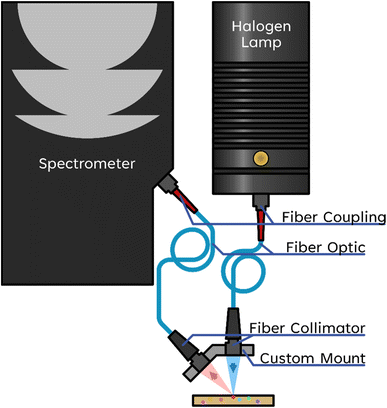
Near infrared spectra were measured using a custom-built instrument in a reflection and backscattering geometry (Fig. 1). A fiber-couple tungsten halogen lamp (Ocean Optics HL-2000-LL-FHSA) was used for illumination. The light is focused on the sample using a collimating lens (Ocean Optics 74-VIS). The beam waist was determined to have a full width at half max of 900 μm. An identical collimating lens and fiber optic cable (Ocean Optics QP600-2-VIS-NIR) are used for collecting the remitted light. The illumination and collection arms are oriented at a 45° angle. The remittance geometry allows for the collection of plastic spectra even when the plastic samples are rough, angled, rounded, or poorly positioned because the spectral data is typically carried via scattered light. The collected signal is measured with an InGaAs-based spectrometer (Ocean Optics NIRQUEST+1.7).

Fig. 1 Schematic of the near infrared (NIR) instrument. A broadband light source is focused onto a sample and the remitted light is collected at a 45° angle between the illumination and collection sources. The collected light is sent to a spectrometer for measurement, as described in the text.

Samples were placed on a stone for data collection, with data acquired from single particles of each sample. A stone was chosen that had a matching NIR spectrum to that of sand. Using a stone instead of sand allows for quicker sample positioning, exchange, and reduces the risk of cross-contamination. Dark and reference spectra were measured before the samples. The absorbance, A, was calculated according to eqn (1), where R_sample represents the intensity of the sample, R_reference is the intensity of the stone, and R_dark is the output of the spectrometer with the input aperture blocked.

Second order polynomial fitting was used for baseline correction of the spectra. A Fourier filter was applied to remove some diffractive noise. This process involves applying a half-life-based exponential decay with a cut-on at ±0.5 ps in the Fourier domain. The half-life of the exponential decay is 0.2 ps. i.e., the signal at ±0.7 ps is reduced by half. The spectral acquisition time was 100 ms.

2.3 Augmentation and classification

NIR spectra of plastics and environmental interferent materials were collected. They were categorized as ABS, nylon, PET, PE, PLA, PP, PS, PVC, rubber, plant-based, and water, as described above. Water spectra were collected by measuring a wetted stone, similar to a wet sand environment found on a beach. A total of 119 plastic spectra were collected, 8 plant-based spectra, 1 water spectrum, and 5 blank spectra. The blank spectra were augmented with uncorrelated Gaussian noise only.

Using the basis set of plastic and interferents (water and plant) spectra, two larger training sets were generated in parallel via data augmentation (Fig. 2). The plastic spectra were combined with Gaussian noise at multiple signal-to-noise levels. The ratio of the standard deviation of the noise to the peak height of the signal was between 0 and 0.4. After adding noise, one set of the spectrum was saved as is, while the second set was created by combining the spectrum with water and/or plant spectra at varying ratios from 0 to 4. In this way, there are two training sets with identical basis sets and noise, but that differ in the presence of interferent spectra. In all, 48 000 × 2 spectra were generated for training the algorithms and 48 000 × 2 spectra were generated for testing. An additional set of 48 000 × 2 spectra with Gaussian noise ratios ranging from 0 to 2 was generated for further characterization of the models' performance at high noise levels.

Fig. 2 Schematic overview of the data generation and augmentation process for near-infrared (NIR) spectra. The measured spectra include plastic spectra without interferents and interferent spectra from water and plant matter. Synthetic noise is added through Gaussian noise simulations. The augmented training set and testing set, include noisy spectra with and without interferents. The measured benchmarking set comprises spectra of plastics collected in the presence of water and/or plant matter, providing real-world validation for the model.

This comprehensive dataset ensures robust training and benchmarking, allowing the model to handle real-world spectral challenges effectively.

A second order polynomial background was subtracted from each spectrum. The polynomial was fit to baseline points between 7550 cm⁻¹ to 7850 cm⁻¹ and 9550 cm⁻¹ to 10 500 cm⁻¹. Each NIR spectrum was normalized to a maximum of 1 between the range of 6500 cm⁻¹ to 9200 cm⁻¹, which is the region that contains the CH stretch first overtone + CH bend combination band (ν⁽¹⁾_CH + δ_CH) and the CH stretch second overtone band (ν⁽²⁾_CH), among other identifying features.³³ The wavelength information was discarded as each spectrum is identical in this regard. The 512 points of the spectra were used as predictor variables for classification. Each observation (spectrum) was labeled with the material category. Classifier algorithms were trained in MATLAB R2023b. For both the noise-only and noise-plus-interferent-augmented data sets, linear discriminant (LDA), support vector machine (SVM), k-nearest neighbor (KNN), and neural network (NN) classifier models were trained.

2.4 Non-synthetic testing data

In addition to generated testing data, further testing spectra were collected by measuring NIR spectra of plastics in the presence of interferent sources. This was achieved by placing plastic samples on top of or next to plant material to generate mixed spectra. Additionally, some samples had water added to the plant material, the stone, or on top of the plastic. In this way, 59 spectra were collected to benchmark the trained models. A photograph of one such sample is included in the Section S1.†

3 Results and discussion

3.1 NIR spectra

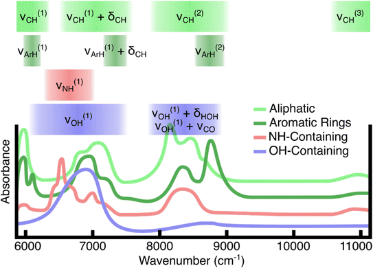
The collected NIR spectra are characterized by a set of spectral features which are overtones or combinations of fundamental molecular vibrations (Fig. 3). Different plastics have identifying spectra because the unique chemical composition for each plastic contributes to the myriad of higher order combinations, overtones, and Fermi resonances.³³ However, the spectral bands can generally be characterized by a handful of features. For aliphatic hydrocarbons, the basis of many consumer plastics, the CH stretch second overtone (ν⁽²⁾_CH) as well as the combination band of the CH stretch first overtone and the CH bending fundamentals (ν⁽¹⁾_CH + δ_CH) are well suited for classifying plastics with specificity. Hydrocarbons with aromatic rings show the aliphatic bands as well as narrower peaks which are blueshifted in the same regions. Plastics which contain NH groups show first-overtone stretching features (ν⁽¹⁾_NH) in a slightly lower energy region than the CH stretch–bend combination band. Finally, OH groups present in water and carbohydrates (plant-material) show broad first overtone stretching features (ν⁽¹⁾_OH) as well as combination bands between the stretches and water bending (ν⁽¹⁾_OH + δ_HOH) in the case of water, or alcohol CO stretches (ν⁽¹⁾_OH + ν_CO) in the case of carbohydrates.

Fig. 3 Schematic of the notable peaks in the NIR region. Primary identifying regions for the plastics are the combination band of the CH stretch first overtone and the CH bend (ν⁽¹⁾_CH + δ_CH) as well as the CH stretch second overtone (ν⁽¹⁾_CH). These and the aromatic CH bands are shown in green. The water spectral features are shown in blue, and the NH spectral features are shown in red.

Fig. 4 contains averaged experimental spectra of each plastic measured. Plastics containing aromatic rings in their polymer structure are characterized primarily by their blueshifted peaks in the first (ν⁽¹⁾_ArH) and second (ν⁽²⁾_ArH) overtone region with respect to the plastics lacking aromatic rings. The presence of both aliphatic and aromatic CH in these plastics results in a “doublet” in the second overtone region with highly unique spacings and peak ratios. The aliphatic plastics in this study tend to have more variance in the peak structure and more small peaks in the overtone region as compared to the aromatic polymers. One distinguishing feature of the nylon spectra is the NH stretch overtone (ν⁽¹⁾_NH), which is centered around 6500 cm⁻¹. Both water and plant/wood spectra are dominated by OH contributions, distinguishable primarily in the lower-energy portions of the spectral range. Even though there is an abundance of CH and other aliphatic groups in polysaccharides, these do not contribute strongly to the plant spectra. This may be a combination of lower absorption strength as well as the presence of water in wood and paper material.

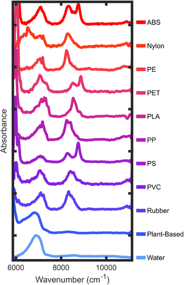Fig. 4 Averaged absorbance spectra of each category of material. Frequency in cm⁻¹ is on the x-axis and absorbance is on the y-axis. The definition of each plastic is included in the Methods.

3.2 Classification algorithms

The MATLAB 2023b classification learner was used to train classification algorithms using the labeled training data set. Algorithms were selected based on those which are common and perform well in other classification studies.^31,35,41,42 Many variations of SVM, KNN, neural network, and discriminant models were trained. The highest performing algorithms on the training set were the cubic SVM (SVM³) and the wide neural network (WNN). The wide neural network consisted of a single fully connected layer with 100 nodes, a ReLU activation function, and was trained over 1000 iterations. The cubic SVM and wide neural network were tested on two testing data sets, one of which had water and plant added in. The accuracy of these algorithms is summarized in Table 1.

Table 1 Classification performance of the top-performing models on test data that has been augmented with noise and augmented with and without environmental interferent spectra. SVM³ is the cubic support vector machine model and WNN is the wide neural network model

Algorithm	Accuracy on test data with noise only	Accuracy on test data with noise and interferents
SVM^3	99.8	52.3
SVM^3 trained with interferent augmentation	99.5	98.5
WNN	99.6	53.3
WNN trained with interferent augmentation	99.4	98.4

---

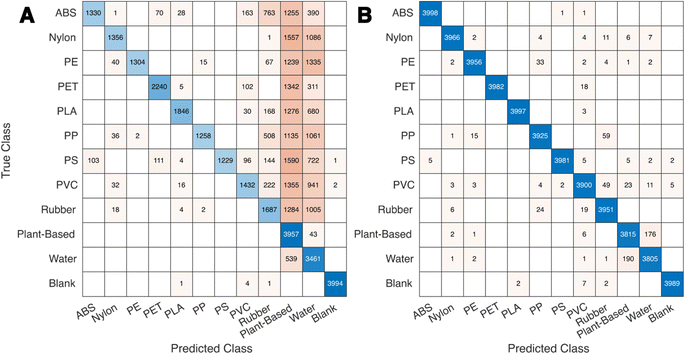
The cubic support vector machine (SVM³) models and wide neural network (WNN) models retain a high degree of accuracy when transferring from the training to the testing data sets which are only augmented with Gaussian noise. The models trained on interferent-augmented data have a slightly worse performance when tested on spectral data augmented with noise only. The interferent-free models are likely more optimized over this feature space because their training sets have four times as many interferent-free spectra as the models trained with interferent augmentation. However, the models trained with interferent augmentation exhibit minimal performance losses when transferring to an interferent-rich testing set, while the interferent-free models experience a significant drop-off. This accuracy reduction is characterized by a sharp rise in the false-positive rate of plant-based, water, and rubber classification (Fig. 5).

Fig. 5 Confusion matrix of the cubic SVM model trained on spectral data augmented with noise only. (Interferent-free model) (A), and the cubic SVM model trained on spectral data augmented with both noise and interferents (B) tested on the synthetic testing set. The x-axis represents the predicted class, while the y-axis represents the true class. True positives are represented by the diagonal elements, indicating correctly classified samples. False positives are shown as off-diagonal elements in a column, where a sample is incorrectly classified into a certain class. False negatives are represented by off-diagonal elements in a row, where a sample is incorrectly excluded from its true class. The inclusion of interferent data during training in the model (B) significantly reduces misclassifications compared to the model (A).

Plant-based and water false positives are rationally explained by the lack of training data for the cubic SVM model that includes plant-based and water interferents. Rubber false positives are more surprising, considering the existence of rubber as an equivalently sampled class in the training set. The rubber basis spectra tend to have a slight upward curve in the baseline towards the red region of the spectrum (Fig. 5). This upward curve may mimic low levels of water or plant-based spectra and be the source of the false positives.

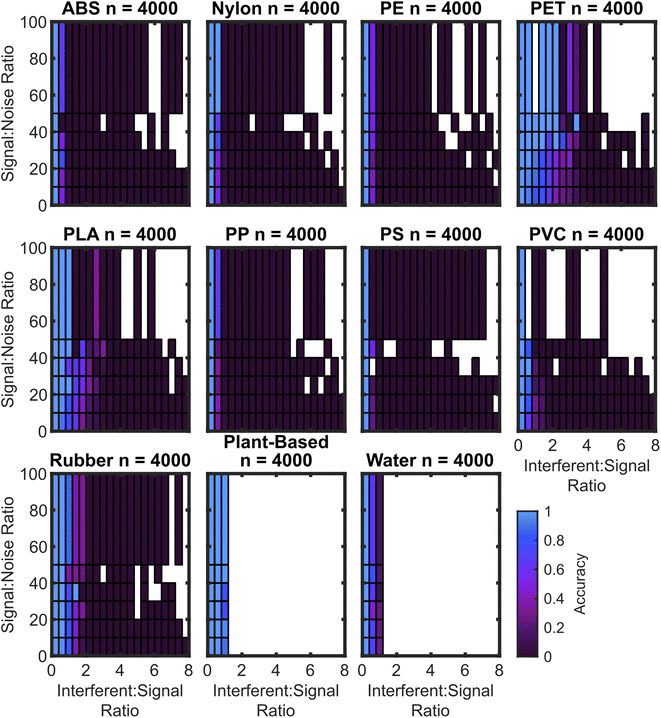
While the confusion matrix gives an overall performance metric, the true positive rate for each plastic depends on the signal-to-noise ratio (SNR) as well as the presence and magnitude of interferent signals, hereafter quantified by the interferent-to-signal ratio (ISR), which is the ratio of the maximum intensity of the plant spectrum plus water spectrum to the maximum intensity of the plastic sample spectrum. The dependence of accuracy on SNR and ISR is shown via a two-dimensional histogram tile plot. Fig. 6 is an annotated form of this plot which identifies four quadrants: high-SNR low-ISR, high-SNR high-ISR, low-SNR low-ISR, and low-SNR high-ISR.

Fig. 6 Two-dimensional histogram tiles illustrating the performance of the cubic SVM model trained on spectral data augmented with both noise and interferents for polypropylene. Signal-to-noise ratios (SNR) are shown on the y-axis, interferent-to-signal ratios (ISR) on the x-axis, and accuracy is depicted by the color scale. White regions indicate areas without data. A sample spectrum from each quadrant of the plot is included, with frequency (cm⁻¹) on the x-axis and absorbance on the y-axis. As SNR decreases, spectral features become increasingly unclear by noise, while higher ISR values reflect greater overlap of spectral features by those of water and plant matter.

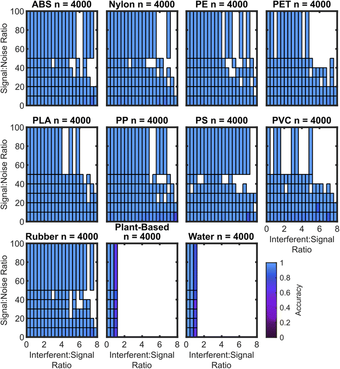
As expected, the algorithms trained with synthetic interferent data perform optimally at high SNR and low ISR, with the worst performance at low SNR and high ISR. For the SVM³+I model, the accuracy drop is minimal. The performance of the SVM³+I algorithm for all plastics is shown in Fig. 7, which can be compared to the SVM³ model in Fig. 8.

Fig. 7 Two-dimensional histogram tiles showing the performance of the cubic SVM model trained on spectral data augmented with both noise and interferents for each plastic, with signal-to-noise ratios (SNR) on the y-axis, interferent-to-signal ratios (ISR) on the x-axis, and accuracy represented by the color scale. White regions have no data.

Fig. 8 Two-dimensional histogram tiles showing the performance of the cubic SVM model trained on spectral data augmented with noise only for each plastic, with signal-to-noise ratios (SNR) on the y-axis, interferent-to-signal ratios (ISR) on the x-axis, and accuracy represented by the color scale. White regions have no data.

The algorithm cubic SVM model trained on spectral data augmented with both noise and interferents generally shows small accuracy drops at low SNR and high ISR. Some plastics lack >50 SNR spectra due to the lack of these spectra in the basis set.

Fig. 7 also does not have ISR data greater than 1 for the water and plant-based spectra. This is because water and plant-based spectra are both used as interferents, so a spectrum that is 1 part nylon to 2 parts water should be classified as nylon, but a spectrum that is 1 part plant to 2 parts water should be classified as water.

In contrast to the model trained on augmentation of interferent data, the model trained on augmentation of noise data performs well only when the ISR is low. The exception to this rule is the PET which maintains accuracy to a ISR of approximately 2. The rubber and PLA samples maintain accuracy towards ISRs of approximately 1. Notably, both rubber and PET have baselines that curve upward towards the red region of the spectrum, which is similar to the effect caused by lower levels of plant and water spectra. While the false positive rate for rubber shown in Fig. 4 is attributed to this curve, the curving baseline also appears to confer higher true positive rates for these moderate ISR levels. The curved baselines may be due to spectral features or non-ideal baseline subtraction. However, automated baseline subtraction of the plastic spectra is very challenging to improve because the spectral regions that are not overlapped by any plastic peaks are very narrow. It may not be possible to improve upon polynomial subtraction without a wider detector range or different baseline techniques. Some prior approaches have used first derivatives to reduce baseline effects, but this can also confer greater noise sensitivity.^32,39

3.3 Testing classification algorithms on measured sample data

In this manuscript, authentic data refers to plastic spectra collected in the presence of water and/or plant material, in contrast to synthetic data, which is plastic spectra that has been augmented with linear additions of plant and/or water spectra. Testing the trained algorithms on synthetic data is useful in characterizing the models and diagnosing their shortcomings, but these models must also work on measured samples. It is possible that environmental and plastic spectra may not linearly combine. Therefore, new spectra were collected with plastic samples and the interferents. We considered the interferents as both neighboring plant matter and water within the field of view of the spectrometer and as well as those adsorbed onto the plastic surfaces. Neighboring plant matter and water in the field of light contribute to obvious spectral interference due to their strong vibrational features. When plant matter or water is adsorbed onto the plastic surface, the detection signal returning to the spectrometer can originate from both the plastic and the interferent, thereby creating a significant interference scenario. However, if the light becomes trapped within the plant matter or water and does not reach the plastic, this scenario will not be applicable, as no meaningful plastic-specific signal will be returned. Similarly, if the plastic is positioned on top of plant matter or water and the light reaches both materials, the resulting signal will contain features from the interferents and the plastic. In such cases, plant- or water-augmented plastic spectra will provide an equivalent representation of the real scenario of interferents impacting microplastic detection.

The cubic SVM models trained on spectral data augmented with noise only and on noise and interferents were evaluated on these authentic samples (Fig. 9).

Fig. 9 Confusion matrix of the cubic SVM model trained on spectral data augmented with noise only. (Interferents-free model) (A), and the cubic SVM model trained on spectral data augmented with both noise and interferents (B) tested on the authentic testing set. The x-axis represents the predicted class, while the y-axis represents the true class. True positives are represented by the diagonal elements, indicating correctly classified samples. False positives are shown as off-diagonal elements in a column, where a sample is incorrectly classified into a certain class. False negatives are represented by off-diagonal elements in a row, where a sample is incorrectly excluded from its true class. The model (B) shows the reduced misclassifications compared to the model (A).

The accuracy of the cubic SVM model trained on spectral data augmented with noise only and cubic SVM model trained on spectral data augmented with both noise and interferents models are 40.7% and 86.4%, respectively. This is a drop in performance with respect to the synthetic testing data (Table 1), but the model with interferent augmentation performs significantly better than the interferent-free model. The primary false positives for the interferent-free model are water, plant-based, and rubber. This matches the set of false positives from the synthetic testing set. Interestingly, the model trained on interferents also suffers from a small number (3) of rubber false positives. It is likely that the water and plant levels are higher in some of the testing data than they are in the training data. This may cause differences in polynomial background subtraction which could result in the rubber false positives. This may be further addressed by increasing the plant and water levels in the training set.

3.4 Signal to noise ratio and particle size determination

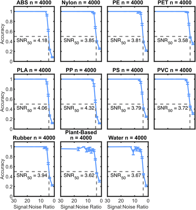
To further characterize the model accuracy related to the SNR, an additional pair of testing data sets were created with augmented noise to signal ratios. This new testing set provides more sample spectra at low SNR, which allows for statistics about the accuracy of the algorithms in this regime. Fig. 10 shows the accuracy of the SVM³+I algorithm on the noisy spectra with interferents over a range of SNRs.

Fig. 10 Accuracy of the cubic SVM model trained on interferents evaluated on noisy data with added interferents as the testing dataset, plotted across different signal-to-noise ratios (SNRs). Data is plotted as a line plot of histogram data with the horizontal axis representative of the histogram bin centers. Error bars are standard deviations determined by bootstrapping the accuracy estimates 100 times with 50% of the data each time. Gray dashed lines indicate the SNR at which the model is 50% accurate as determined via linear interpolation.

Fig. 10 shows that the cubic SVM model trained on interferents has nearly perfect identification capabilities above an SNR of 7.5. The performance of the algorithm drops to 50% at an SNR of around 4 for each plastic. Interestingly, the training data had a maximum added noise level at an SNR of 2.5. Therefore, this performance may be near the limit of possibility for this set of samples. To get a better sense of the practical implications of SNR on classifying plastics in the field, the SNRs of neat plastics of a range of particle sizes were determined. Fig. 11 summarizes the correlation between SNR and particle size with the described NIR instrument.

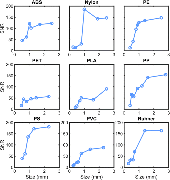Fig. 11 Variation of SNR with size for different plastic types. Each subplot represents a different plastic type, with SNR on the y-axis and size in mm on the x-axis.

The SNR scaling displayed in Fig. 11 shows that many of the plastic materials maintain very high SNR levels (>30) even at sizes as low as 0.5 mm or less. The samples which tend to have lower SNR are approaching an SNR of 10 at sizes of around 0.5 mm. Based on the performance measurements in Fig. 10, this should correspond to accuracies of around 100% on most plastics for 0.5 mm particles, even with high levels of interferent signal.

4 Discussion

Despite the success, there are many possibilities for improvement in performance. The neoprene rubber false positives suggest a better baseline cleaning methodology may be necessary, which could involve data collection at a wider spectral range. Many prior studies have incorporated first derivatives in order to enhance differences and help remove baselines, however these may introduce more sensitivity to low signal-to-noise conditions.^32,39 Signal-to-noise can be further improved by reducing the spot size or using longer acquisitions, this particularly when measuring smaller or dark-colored samples. Given that integration times can be dynamically changed, adaptive-sampling methods can be further implemented to produce spectra with uniform signal-to-noise ratios. In the present work, the ∼1 mm spot size was designed to add robustness for the possibility of field use, where source and detection optics can become partially misaligned.

If signal-to-noise can be improved by reducing the spot size or using longer acquisitions, this would also help with smaller or dark-colored samples.

In this study, black colored plastics were not considered due to their strong absorption and low reflectance properties. These challenges have been discussed in recent studies, emphasizing and exploring the need of innovative advanced vibrational analysis.^43,44

One other shortcoming in the present model is the lack of categorization for mixed plastics. While not the focus of this work, the data augmentation method described in this manuscript is compatible with machine learning techniques that classify mixed plastics. Another possible avenue for improvement in model transferability between synthetic and authentic data could be augmentation techniques beyond linear combinations of spectra. For FTIR, explainable machine learning models have proven to be a superior augmentation method, though not demonstrated in the context of environmental contaminants.³⁵ One additional shortcoming of infrared based classification is the difficulty of collecting spectra of samples submerged in water. Spectra of immersed plastics would likely contain too much water contamination to be successfully classified. Furthermore, plants and water represent an important but small subset of the many potential spectral contaminants, and future models could also include the ability to detect or ignore many other materials. For example, some plastic dyes and soil materials can produce additional peaks in the NIR range. As others have suggested, future classification algorithms should be tested and trained on weathered plastics that may have chemical changes or contaminants not explored in this work.^32,34

Naturally, machine learning models need to be trained and evaluated in an iterative approach, oscillating between exposing model shortcomings with real-world data and refining the algorithm to include the new information.

5 Conclusions

The detection of microplastics in the field would be an important component to developing future quantification standards. Currently, microplastic surveys typically rely on sample transportation and several processing steps. Achieving the goal of mobile sensing requires plastic identification technology that is cost-effective, compact in size, sensitive to different materials, and can filter out common interferents with software rather than complicated and time-consuming physical processing of samples. NIR spectroscopy has both compactness and sensitivity, and machine learning completes the requirements by conferring robustness to sample identification despite water and plant environmental interferents. In this work, we demonstrated that augmentation of a limited spectral basis set with interferent spectra significantly improves machine learning performance on real-world data classification, going from 40.7% accuracy to 86.4%.

Future work should focus on developing machine learning models that incorporate a wider range of spectral interferences, including dyes, soil materials, and other environmental substances. Testing the current machine learning model with datasets of weathered plastics is also essential for checking the classification accuracy and robustness. Finally, achieving real-time, in-field plastic detection will require further optimization of compact NIR spectroscopy systems and machine learning algorithms to ensure high accuracy under diverse environmental conditions. By addressing these challenges, future advancements can direct the research toward more effective environmental monitoring and plastic identification technologies.

Data availability

The data used in this work is openly available via the Texas Data Repository (https://doi.org/10.18738/T8/KPE70S).

Conflicts of interest

The authors have no conflict to report.

Acknowledgements

This work is supported by the Welch Foundation (F-1891), the Matagorda Bay Mitigation Trust, and the UT Austin Office of the Vice President for Research, Scholarship and Creative Endeavors. We would also like to thank Julius Rivera, and Shreya Arvind for assisting with plastic acquisition and insightful discussion on microplastics.

References

1. OECD, Global Plastic Outlook, 2019,  DOI:10.1787/c0821f81-en.
2. D. K. A. Barnes, F. Galgani, R. C. Thompson and M. Barlaz, Accumulation and Fragmentation of Plastic Debris in Global Environments, Philos. Trans. R. Soc., B, 2009, 364(1526), 1985–1998,  DOI:10.1098/rstb.2008.0205.
3. M. A. Browne, P. Crump, S. J. Niven, E. Teuten, A. Tonkin, T. Galloway and R. Thompson, Accumulation of Microplastic on Shorelines Woldwide: Sources and Sinks, Environ. Sci. Technol., 2011, 45(21), 9175–9179,  DOI:10.1021/es201811s.
4. C. M. Rochman, M. A. Browne, A. J. Underwood, J. A. van Franeker, R. C. Thompson and L. A. Amaral-Zettler, The Ecological Impacts of Marine Debris: Unraveling the Demonstrated Evidence from What Is Perceived, Ecology, 2016, 97(2), 302–312,  DOI:10.1890/14-2070.1.
5. N. K. Y. Susanti, A. Mardiastuti and Y. Wardiatno, Microplastics and the Impact of Plastic on Wildlife: A Literature Review, IOP Conf. Ser.: Earth Environ. Sci., 2020, 528(1), 012013,  DOI:10.1088/1755-1315/528/1/012013.
6. J. Carlin, C. Craig, S. Little, M. Donnelly, D. Fox, L. Zhai and L. Walters, Microplastic Accumulation in the Gastrointestinal Tracts in Birds of Prey in Central Florida, USA, Environ. Pollut., 2020, 264, 114633,  DOI:10.1016/j.envpol.2020.114633.
7. X. Chang, Y. Fang, Y. Wang, F. Wang, L. Shang and R. Zhong, Microplastic Pollution in Soils, Plants, and Animals: A Review of Distributions, Effects and Potential Mechanisms, Sci. Total Environ., 2022, 850, 157857,  DOI:10.1016/j.scitotenv.2022.157857.
8. M. Cole, P. Lindeque, C. Halsband and T. S. Galloway, Microplastics as Contaminants in the Marine Environment: A Review, Mar. Pollut. Bull., 2011, 62(12), 2588–2597,  DOI:10.1016/j.marpolbul.2011.09.025.
9. L. A. Kesner, Z. A. Piskulich, Q. Cui and Z. Rosenzweig, Untangling the Interactions between Anionic Polystyrene Nanoparticles and Lipid Membranes Using Laurdan Fluorescence Spectroscopy and Molecular Simulations, J. Am. Chem. Soc., 2023, 145(14), 7962–7973,  DOI:10.1021/jacs.2c13403.
10. W. Tian, P. Song, H. Zhang, X. Duan, Y. Wei, H. Wang and S. Wang, Microplastic Materials in the Environment: Problem and Strategical Solutions, Prog. Mater. Sci., 2023, 132, 101035,  DOI:10.1016/j.pmatsci.2022.101035.
11. L. D. K. Kanhai, K. Gardfeldt, T. Krumpen, R. C. Thompson and I. O'Connor, Microplastics in Sea Ice and Seawater beneath Ice Floes from the Arctic Ocean, Sci. Rep., 2020, 10(1), 5004,  DOI:10.1038/s41598-020-61948-6.
12. J. Li, H. Liu and J. Paul Chen, Microplastics in Freshwater Systems: A Review on Occurrence, Environmental Effects, and Methods for Microplastics Detection, Water Res., 2018, 137, 362–374,  DOI:10.1016/j.watres.2017.12.056.
13. A. L. Andrady, The Plastic in Microplastics: A Review, Mar. Pollut. Bull., 2017, 119(1), 12–22,  DOI:10.1016/j.marpolbul.2017.01.082.
14. R. Kumar, P. Sharma, C. Manna and M. Jain, Abundance, Interaction, Ingestion, Ecological Concerns, and Mitigation Policies of Microplastic Pollution in Riverine Ecosystem: A Review, Sci. Total Environ., 2021, 782, 146695,  DOI:10.1016/j.scitotenv.2021.146695.
15. V. Hidalgo-Ruz, L. Gutow, R. C. Thompson and M. Thiel, Microplastics in the Marine Environment: A Review of the Methods Used for Identification and Quantification, Environ. Sci. Technol., 2012, 46(6), 3060–3075,  DOI:10.1021/es2031505.
16. J. C. Prata, J. P. da Costa, A. C. Duarte and T. Rocha-Santos, Methods for Sampling and Detection of Microplastics in Water and Sediment: A Critical Review, TrAC, Trends Anal. Chem., 2019, 110, 150–159,  DOI:10.1016/j.trac.2018.10.029.
17. H. Lee, S. Kim, A. Sin, G. Kim, S. Khan, M. N. Nadagouda, E. Sahle-Demessie and C. Han, Pretreatment Methods for Monitoring Microplastics in Soil and Freshwater Sediment Samples: A Comprehensive Review, Sci. Total Environ., 2023, 871, 161718,  DOI:10.1016/j.scitotenv.2023.161718.
18. A. P. M. Michel, A. E. Morrison, V. L. Preston, C. T. Marx, B. C. Colson and H. K. White, Rapid Identification of Marine Plastic Debris via Spectroscopic Techniques and Machine Learning Classifiers, Environ. Sci. Technol., 2020, 54(17), 10630–10637,  DOI:10.1021/acs.est.0c02099.
19. D. Schymanski, C. Goldbeck, H.-U. Humpf and P. Fürst, Analysis of Microplastics in Water by Micro-Raman Spectroscopy: Release of Plastic Particles from Different Packaging into Mineral Water, Water Res., 2018, 129, 154–162,  DOI:10.1016/j.watres.2017.11.011.
20. Y. Xu, Q. Ou, M. Jiao, G. Liu and J. P. Van Der Hoek, Identification and Quantification of Nanoplastics in Surface Water and Groundwater by Pyrolysis Gas Chromatography–Mass Spectrometry, Environ. Sci. Technol., 2022, 56(8), 4988–4997,  DOI:10.1021/acs.est.1c07377.
21. J.-L. Xu, K. V. Thomas, Z. Luo and A. A. Gowen, FTIR and Raman Imaging for Microplastics Analysis: State of the Art, Challenges and Prospects, TrAC, Trends Anal. Chem., 2019, 119, 115629,  DOI:10.1016/j.trac.2019.115629.
22. R. Lenz, K. Enders, C. A. Stedmon, D. M. A. Mackenzie and T. G. Nielsen, A Critical Assessment of Visual Identification of Marine Microplastic Using Raman Spectroscopy for Analysis Improvement, Mar. Pollut. Bull., 2015, 100(1), 82–91,  DOI:10.1016/j.marpolbul.2015.09.026.
23. S. Primpke, P. A. Dias and G. Gerdts, Automated Identification and Quantification of Microfibres and Microplastics, Anal. Methods, 2019, 11(16), 2138–2147,  10.1039/C9AY00126C.
24. V. H. da Silva, F. Murphy, J. M. Amigo, C. Stedmon and J. Strand, Classification and Quantification of Microplastics (<100 μm) Using a Focal Plane Array–Fourier Transform Infrared Imaging System and Machine Learning, Anal. Chem., 2020, 92(20), 13724–13733,  DOI:10.1021/acs.analchem.0c01324.
25. X. Yan, Z. Cao, A. Murphy, Y. Ye, X. Wang and Y. Qiao, FRDA: Fingerprint Region Based Data Augmentation Using Explainable AI for FTIR Based Microplastics Classification, Sci. Total Environ., 2023, 896, 165340,  DOI:10.1016/j.scitotenv.2023.165340.
26. B. Zhao, R. E. Richardson and F. You, Advancing Microplastic Analysis in the Era of Artificial Intelligence: From Current Applications to the Promise of Generative AI, Nexus, 2024, 1(4), 100043,  DOI:10.1016/j.ynexs.2024.100043.
27. Y. Liu, W. Yao, F. Qin, L. Zhou and Y. Zheng, Spectral Classification of Large-Scale Blended (Micro)Plastics Using FT-IR Raw Spectra and Image-Based Machine Learning, Environ. Sci. Technol., 2023, 57(16), 6656–6663,  DOI:10.1021/acs.est.2c08952.
28. B. R. Coleman, An Introduction to Machine Learning Tools for the Analysis of Microplastics in Complex Matrices, Environ. Sci.: Processes Impacts, 2025, 27(1), 10–23,  10.1039/D4EM00605D.
29. M. A. Johns, H. Zhao, M. Gattrell, J. Lockhart and E. D. Cranston, Identification of Common Textile Microplastics via Autofluorescence Spectroscopy Coupled with k-Means Cluster Analysis, Analyst, 2024, 149(18), 4747–4756,  10.1039/D4AN00658E.
30. A. Hahn, G. Gerdts, C. Völker and V. Niebühr, Using FTIRS as Pre-Screening Method for Detection of Microplastic in Bulk Sediment Samples, Sci. Total Environ., 2019, 689, 341–346,  DOI:10.1016/j.scitotenv.2019.06.227.
31. A. P. M. Michel, A. E. Morrison, V. L. Preston, C. T. Marx, B. C. Colson and H. K. White, Rapid Identification of Marine Plastic Debris via Spectroscopic Techniques and Machine Learning Classifiers, Environ. Sci. Technol., 2020, 54(17), 10630–10637,  DOI:10.1021/acs.est.0c02099.
32. C. Vidal and C. Pasquini, A Comprehensive and Fast Microplastics Identification Based on Near-Infrared Hyperspectral Imaging (HSI-NIR) and Chemometrics, Environ. Pollut., 2021, 285, 117251,  DOI:10.1016/j.envpol.2021.117251.
33. W. Kaye, Near-Infrared Spectroscopy: I. Spectral Identification and Analytical Applications, Spectrochim. Acta, 1954, 6(4), 257–287,  DOI:10.1016/0371-1951(54)80011-7.
34. C. Zhu, Y. Kanaya, R. Nakajima, M. Tsuchiya, H. Nomaki, T. Kitahashi and K. Fujikura, Characterization of Microplastics on Filter Substrates Based on Hyperspectral Imaging: Laboratory Assessments, Environ. Pollut., 2020, 263, 114296,  DOI:10.1016/j.envpol.2020.114296.
35. X. Yan, Z. Cao, A. Murphy, Y. Ye, X. Wang and Y. F. R. D. A. Qiao, Fingerprint Region Based Data Augmentation Using Explainable AI for FTIR Based Microplastics Classification, Sci. Total Environ., 2023, 896, 165340,  DOI:10.1016/j.scitotenv.2023.165340.
36. J. Weisser, T. Pohl, M. Heinzinger, N. P. Ivleva, T. Hofmann and K. Glas, The Identification of Microplastics Based on Vibrational Spectroscopy Data – A Critical Review of Data Analysis Routines, TrAC, Trends Anal. Chem., 2022, 148, 116535,  DOI:10.1016/j.trac.2022.116535.
37. A. Paul, L. Wander, R. Becker, C. Goedecke and U. Braun, High-Throughput NIR Spectroscopic (NIRS) Detection of Microplastics in Soil, Environ. Sci. Pollut. Res., 2019, 26(8), 7364–7374,  DOI:10.1007/s11356-018-2180-2.
38. Y. Liu, Z. Huo, M. Huang, R. Yang, G. Dong, Y. Yu, X. Lin, H. Liang and B. Wang, Rapid Detection of Microplastics in Chicken Feed Based on near Infrared Spectroscopy and Machine Learning Algorithm, Spectrochim. Acta, Part A, 2025, 329, 125617,  DOI:10.1016/j.saa.2024.125617.
39. Q. Duan and J. Li, Classification of Common Household Plastic Wastes Combining Multiple Methods Based on Near-Infrared Spectroscopy, ACS ES&T Eng., 2021, 1(7), 1065–1073,  DOI:10.1021/acsestengg.0c00183.
40. T. M. Karlsson, H. Grahn, B. van Bavel and P. Geladi, Hyperspectral Imaging and Data Analysis for Detecting and Determining Plastic Contamination in Seawater Filtrates, J. Near Infrared Spectrosc., 2016, 24(2), 141–149,  DOI:10.1255/jnirs.1212.
41. M. Kedzierski, M. Falcou-Préfol, M. E. Kerros, M. Henry, M. L. Pedrotti and S. Bruzaud, A Machine Learning Algorithm for High Throughput Identification of FTIR Spectra: Application on Microplastics Collected in the Mediterranean Sea, Chemosphere, 2019, 234, 242–251,  DOI:10.1016/j.chemosphere.2019.05.113.
42. H. de M. Back, E. C. Vargas Junior, O. E. Alarcon and D. Pottmaier, Training and Evaluating Machine Learning Algorithms for Ocean Microplastics Classification through Vibrational Spectroscopy, Chemosphere, 2022, 287, 131903,  DOI:10.1016/j.chemosphere.2021.131903.
43. K. Zhou, S.-K. Oh, W. Pedrycz, J. Qiu, Z. Fu and B.-G. Ryu, Design of Data Feature-Driven 1D/2D Convolutional Neural Networks Classifier for Recycling Black Plastic Wastes through Laser Spectroscopy, Adv. Eng. Inform., 2022, 53, 101695,  DOI:10.1016/j.aei.2022.101695.
44. N. Stavinski, V. Maheshkar, S. Thomas, K. Dantu and L. Velarde, Mid-Infrared Spectroscopy and Machine Learning for Postconsumer Plastics Recycling, Environ. Sci.: Adv., 2023, 2(8), 1099–1109,  10.1039/D3VA00111C.

---

Footnote

† Electronic supplementary information (ESI) available: Images of plastic sources used in this work as well as the 2D beam profile of the NIR instrument. See DOI: https://doi.org/10.1039/d4su00612g

---