An automatic segmentation and quantification method for austenite and ferrite phases in duplex stainless steel based on deep learning
Lun
Che
a,
Zhongping
He
 *a,
Kaiyuan
Zheng
a,
Xiaotian
Xu
a and
Feng
Zhao
b
aCollege of Mechanical Engineering, Chengdu University, China. E-mail: chelun2821913044@gmail.com; hezhongping@cdu.edu.cn
bInstitute of Advanced Study, Chengdu University, China
First published on 2nd December 2024
Abstract
Traditional microstructural analysis and phase identification largely rely on manual efforts, inevitably affecting the consistency and accuracy of the results. Historically, the identification of ferrite and retained austenite phases and the extraction of grain information have predominantly been conducted by experts based on their experience. This process is not only time-consuming and labor-intensive but also prone to discrepancies due to the subjective nature of expert judgment. With the continuous advancement of deep learning technologies, new solutions for the classification and analysis of microstructures have emerged. This study proposes a microstructural segmentation method for dual-phase steel based on the Mask R-CNN deep learning model, which can quickly and accurately segment ferrite and retained austenite phases in dual-phase steel subjected to different heat treatment temperatures, enabling quantitative analysis of grain information. First, lightweight dual-phase steel is subjected to heat treatments at five different temperatures, and electron microscope images are obtained as training and testing data for the network. Through data preprocessing, annotation, and augmentation, a microstructural image dataset is constructed. Subsequently, the Mask R-CNN deep learning model is employed to recognize and segment the microstructural dataset of dual-phase steel. From the mask images output by the model, quantitative parameters such as the volume fraction and average grain size of ferrite and retained austenite are successfully extracted. Furthermore, the approach demonstrates high portability and applicability, particularly relying on a small sample dataset.
1. Introduction
As the demand for material performance continues to increase, high-performance metal materials have garnered extensive attention and application. Fe–C–Mn–Al dual-phase steel is a novel metal material characterized by high strength, high ductility, and high toughness, finding broad application in aerospace, automotive industries, and other fields. In the application of Fe–C–Mn–Al dual-phase steel, microstructure is one of the key factors determining its mechanical properties.1–5 Ferrite, with its good ductility, serves as the primary phase in dual-phase lightweight steel, endowing the steel with excellent plastic deformation capability. Ferrite influences the grain size and content of austenite; as the volume fraction of ferrite increases, the tensile strength and yield strength increase, while the elongation after fracture shows an opposite trend. Austenite is the main deformation strengthening phase in lightweight steel, and the size and fraction of austenite particles significantly impact the mechanical properties of lightweight steel.6–9 Therefore, accurate identification and quantification of the microstructure in Fe–C–Mn–Al dual-phase steel are of significant research importance. Traditional methods for microstructure identification often require manual intervention,10,11 which is time-consuming and labor-intensive and may involve a degree of subjectivity between different samples. In recent years, the application of machine learning in the field of materials science has grown significantly.12,13 Researchers have begun employing neural network-based methods to automatically identify and classify the microstructures of metallic materials.14–17 Neural network models, with their excellent learning and generalization capabilities, can quickly and accurately classify and predict large datasets, offering broad application prospects. In this context, convolutional neural networks (CNNs)18 have become widely used methods for tasks such as phase classification and identification of microstructures in metallic materials. Azimi et al.19 proposed a method using fully convolutional neural networks (FCNNs) for pixel segmentation, employing a majority voting scheme, which achieved a classification accuracy of 93.94% for steel microstructures. CNNs can automatically extract high-level features from data, thereby achieving tasks such as image classification and object detection, and have been extensively applied in the field of materials science, including the recognition and segmentation of alloy microstructures and defect detection. M. R. Awan et al.20 proposed a deep learning-based crack identification technique, using preprocessed images and the VGG-16 (ref. 21) network model to accurately identify surface cracks in laser-nitrided Ti–6Al–4V materials, achieving an accuracy exceeding 98%. A. R. Durmaz et al.22 employed multidisciplinary deep learning methods to segment micrographs and infer microstructures, achieving 90% accuracy in the segmentation of lath bainite in complex phase steel using various U-Net23 architectures. Zhao et al.24 completed the identification of 2275 images of 15 different microstructures in titanium alloys, utilizing steps such as dataset preparation, image preprocessing, model construction, and parameter tuning, and performed image segmentation on morphologically processed images based on the U-Net23 network.However, traditional CNNs have some issues, such as insufficient accuracy in object segmentation and localization and weak differentiation capability for microstructural parts with different sizes, shapes, and orientations.25 To overcome these problems, some object detection frameworks, such as Faster R-CNN,26 YOLOv5,27 and Mask R-CNN,28 have emerged. In the study,29 researchers customized and trained a Mask R-CNN model implemented in the deep learning framework Detectron2 [https://github.com/facebookresearch/detectron2]30 for the detection and segmentation of martensite–austenite islands (M–A islands), successfully segmenting larger M–A islands. Shen et al.31 used a small number of EBSD images of DP steel and Q&P steel to form ground truth SEM images, then applied the U-Net23 architecture to learn high-level features, performing pixel-level segmentation of the input SEM images, and finally used the OpenCV package to obtain quantitative microstructural information through pixel statistics. Based on the above studies, this research adopts the Mask R-CNN (Mask Region-based Convolutional Neural Network),28 a deep learning-based object detection algorithm, to achieve automatic segmentation of the microstructure of Fe–C–Mn–Al dual-phase steel. Mask R-CNN28 introduces object segmentation on the basis of the object detection framework Faster R-CNN,26 which means it can not only detect objects in the image but also accurately determine their boundaries, thereby achieving more precise object localization. Currently, it has been applied in fields such as face recognition, medical auxiliary detection, and vehicle and pedestrian detection.32–34 In this study, by building a neural network model based on Mask R-CNN,28 we achieved automatic segmentation of the microstructure of Fe–C–Mn–Al dual-phase steel and quantified the image data, obtaining good recognition results on the experimental dataset. Furthermore, the approach demonstrates high portability and applicability, particularly relying on a small sample dataset.
2. Materials and methods
2.1. Dataset acquisition
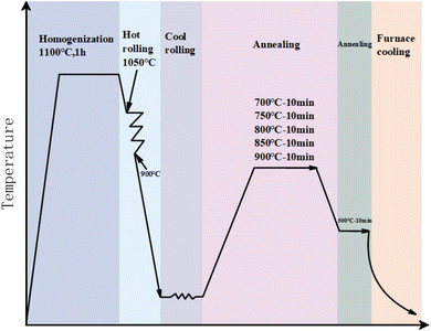
The experimental steel was smelted in a vacuum induction furnace with argon gas protection during the smelting process. A 100 kg ingot was obtained through mold casting, and the chemical composition of the experimental steel was determined by chemical analysis, as shown in Table 1. The ingot was initially homogenized at 1100 °C for 1 hour to eliminate segregation and inclusions. Subsequently, the ingot was hot-rolled to a thickness of 3 mm, with an initial rolling temperature of 1050 °C and a final rolling temperature of 900 °C. The hot-rolled plates were then pickled with 10% HCl at 85 °C mixed with 90% water and dried to remove scale. Any remaining scale was ground off with a grinding wheel to ensure a bright and oxide-free surface. The plates were then cold-rolled to a final thickness of 1.4 mm. The cold-rolled experimental steel was heated to 700 °C, 750 °C, 800 °C, 850 °C, and 900 °C, holding at each temperature for 10 minutes to form a mixture of ferrite and austenite. This was followed by isothermal holding at 500 °C for 10 minutes before the furnace cooled to room temperature. This isothermal quenching treatment, known as isothermal bainite treatment, is employed to suppress carbide formation during the bainite transformation process, thereby retaining austenite at room temperature.35 The heat treatment process is illustrated in Fig. 1.| Element | Weight% |
|---|---|
| C | 0.52 |
| Mn | 11 |
| Al | 5.4 |
| Cr | 1 |
| Fe | Balance |
2.2. Microstructure image dataset generation
After heat treatment, the samples were ground sequentially using 400–2000 grit sandpapers and polished with a W1.5 diamond polishing suspension. They were then etched with a 4% nitric acid alcohol solution and electrolytically polished using a (1![[thin space (1/6-em)]](https://www.rsc.org/images/entities/char_2009.gif) :
:![[thin space (1/6-em)]](https://www.rsc.org/images/entities/char_2009.gif) 10) volume ratio perchloric acid/alcohol mixture as the electrolyte, with an applied voltage of 30 V. Subsequently, a scanning electron microscope (JIB-4700F) was employed to analyze the microstructural information. Utilizing a secondary electron (SE) detector, multiple images were captured along the horizontal and vertical axes at different magnifications to capture the microstructural inhomogeneity induced by the temperature gradient during the cooling process, using different magnifications (including 1000× and 2000× for 10 μm, 3000× and 5000× for 5 μm, and 6000× for 2 μm) to enhance the model's generalization performance and robustness. All images were saved in .tiff format with a resolution of 1280 × 960.
10) volume ratio perchloric acid/alcohol mixture as the electrolyte, with an applied voltage of 30 V. Subsequently, a scanning electron microscope (JIB-4700F) was employed to analyze the microstructural information. Utilizing a secondary electron (SE) detector, multiple images were captured along the horizontal and vertical axes at different magnifications to capture the microstructural inhomogeneity induced by the temperature gradient during the cooling process, using different magnifications (including 1000× and 2000× for 10 μm, 3000× and 5000× for 5 μm, and 6000× for 2 μm) to enhance the model's generalization performance and robustness. All images were saved in .tiff format with a resolution of 1280 × 960.
2.3. Image augmentation and annotation
From scanning electron microscopy (SEM) images of lightweight dual-phase steel samples subjected to five different heat treatments, four images from each treatment were selected, resulting in a total of 20 images. Although the original dataset contains only 20 microstructural images, each image includes a rich representation of ferrite and austenite structures. For instance, at a magnification of 1000× at 10 micrometers, the structural features are quite diverse. We cropped each original image into 16 smaller images of 256 × 256 pixels, resulting in a total of 320 small images that contain various microstructural features, effectively increasing the diversity of the dataset. The annealed steel exhibits a dual-phase microstructure consisting of ferrite (bright gray to white) and austenite (dark gray), as shown in Fig. 2a. To facilitate the annotation of austenite and ferrite using the Labelme36 tool, it is advisable to choose images where the grain boundaries between austenite and ferrite are clearly defined. The Mask R-CNN28 deep model supports transfer learning, which can significantly reduce training time, improve model performance, and decrease the need for large-scale datasets. By utilizing models pre-trained on large datasets, it accelerates model convergence, enhances adaptability, and effectively reduces the risk of overfitting on small datasets. This makes transfer learning particularly valuable in data-scarce fields, such as medical image analysis.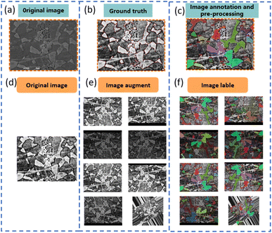 | ||
| Fig. 2 (a) The original microstructure image. (b) Data preprocessing and manual annotation of the ferrite structures in the dataset. (c) The ground truth for each target object (ferrite). (d) The original microstructure image. (e) The image after data augmentation. (f) Using the Labelme36 annotation tool, the ferrite was manually annotated and visualized. | ||
In Mask R-CNN,28 the purpose of data augmentation is similar to its purpose in other deep learning tasks, primarily to enhance the robustness and generalization ability of the model, thereby improving its performance in practical applications. Specifically, data augmentation enables the model to better learn the appearance features and spatial distributions of objects in various scenarios, allowing the model to generalize more effectively to unseen data samples. This reduces the error rate on the test set and helps the model learn more comprehensive and rich feature representations, thereby improving the accuracy and robustness of object detection and instance segmentation.
After preprocessing, the ferrite regions in the images are annotated using the Labelme36 tool. Rectangular or polygonal tools are utilized to ensure accurate annotation of each ferrite region. The annotation results are then saved in JSON file format. Subsequently, the JSON files are converted into masks, allowing for the segmentation of target objects. These masks are saved in a JSON format compliant with the COCO (Common Objects in Context)38 dataset standard for use in model training. Fig. 2a–c illustrate the original image, the image after preprocessing and manual annotation, and the ground truth masks for each target object (ferrite). Through data preprocessing and manual annotation, key structural features in the micrographs are highlighted, providing high-quality data support for subsequent model training.
3. Model design
3.1. Instance segmentation model using Mask R-CNN
Mask R-CNN28 is an object detection and semantic segmentation model based on Faster R-CNN,26 enhanced by the addition of a fully convolutional branch that enables pixel-level segmentation for each detected object, thereby achieving outstanding performance in both object detection and segmentation tasks. Mask R-CNN28 is an extension of Faster R-CNN,26 utilizing its fundamental structure, including the Region Proposal Network (RPN)39 and the object detection network. The RPN, which is the first stage in Mask R-CNN,28 is responsible for proposing potential target regions within the image that may contain objects of interest. The RPN uses a sliding window approach to extract candidate boxes from the feature map and assigns an objectness score to each candidate box to determine the likelihood of containing an object. These candidate boxes are then forwarded to the next processing stage.The candidate boxes filtered by the RPN are input to the object detection network, whose task is to classify and localize the objects within these boxes. In Mask R-CNN,28 ResNet50 or ResNet101 (ref. 40) is typically used as the backbone network for feature extraction, followed by fully connected layers for object classification and bounding box regression. Mask R-CNN28 introduces an additional branch that generates pixel-level masks for each object. This branch operates in parallel with the object detection network, receiving features from the feature extraction stage and generating object masks through a series of convolutional and upsampling operations. These masks represent the precise pixel locations of each object, enabling pixel-level semantic segmentation. The architecture of the Mask R-CNN28 model is illustrated in Fig. 3.
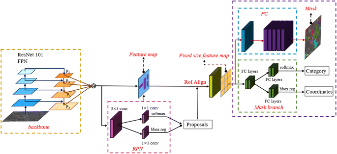 | ||
| Fig. 3 The Mask R-CNN28 architecture with RPN and FPN41 structures. The feature extraction network of Mask R-CNN28 includes both bottom-up and top-down pathways. The FPN layer adopts ResNet-101 (ref. 40) as the backbone network to extract feature maps (P2–P5), which are then fed into the Region Proposal Network (RPN). The candidate bounding boxes filtered by the RPN are sent to the object detection network. Mask R-CNN28 introduces an additional branch for generating pixel-level masks for each target object. | ||
3.2. Hardware and software platform for the Mask R-CNN model
The model training and operations in this study were conducted on Windows 10. The software and hardware environment parameters are as follows: GPU: NVIDIA 3070, Operating System: Windows 10, GPU Driver: NVIDIA GeForce RTX 3070 31.0.15.3713, CUDA: cuda_12.2, CUDNN: cudnn 8.9.2, and PyTorch:42 Torch 2.1.0+cu121.3.3. Training process
Deep learning models for image recognition are composed of complex neural networks. These models analyze the categorical features of each pixel in an image by comparing and analyzing the output results of specific regions with the labeled feature results. To accurately describe different regions of an image, each layer of the neural network is assigned a weight distribution. Training a neural network can be a time-consuming process, and the results are not always optimal. However, transfer learning offers a solution by improving the performance of new tasks through the utilization of prior knowledge obtained from similar or related tasks. This technique is commonly used in deep learning image recognition models to reduce the time required for model training. In this study, a transfer learning approach was employed to initialize the model prior to training, thereby reducing the overall workload of the training process.This study is based on the PyTorch42 deep learning framework, utilizing GPU acceleration for model training. In terms of model architecture, ResNet-101 (ref. 40) is chosen as the backbone network for feature extraction, and the model parameters are initialized using pre-trained Mask R-CNN28 weights from the COCO dataset.43–45 The COCO38 dataset is a large-scale, widely -used benchmark for object detection and instance segmentation, containing annotations for 80 common object categories along with detailed instance segmentation masks. The dataset encompasses complex backgrounds, multi-scale objects, and occlusions. Although the weights trained on the COCO38 dataset are not specifically tailored for microscopic tissue data, the edge feature extraction, multi-scale detection, and complex background segmentation capabilities learned from COCO38 are highly transferable to the task of microscopic image analysis. Subsequently, the dataset comprising 2240 images is inputted into the model, with 70% of the images randomly selected (1568 images) for the training set and the remaining 30% (672 images) for the validation set used for model evaluation. Based on the characteristics of microstructural images of lightweight dual-phase steel, the class is set to 1 (background as the austenite structure). Anchor box sizes are set to 16, 32, 64, 128, and 256, with each size having three aspect ratios (0.5, 1.0, and 2.0), resulting in 256 anchor boxes per image. The Rectified Linear Unit (ReLU) is chosen as the activation function, and the Stochastic Gradient Descent (SGD) method is employed for model optimization. The initial learning rate for model weight parameters is set to 0.001, with a total of 40![[thin space (1/6-em)]](https://www.rsc.org/images/entities/char_2009.gif) 000 iterations for model training. The α weight coefficient and weight decay coefficient are set to 1 and 0.0005, respectively. By appropriately configuring model parameters and training hyperparameters, coupled with enriched samples from data augmentation, the training effectiveness of the model can be effectively enhanced, resulting in improved generalization capability. Model parameters are presented in Table 2.
000 iterations for model training. The α weight coefficient and weight decay coefficient are set to 1 and 0.0005, respectively. By appropriately configuring model parameters and training hyperparameters, coupled with enriched samples from data augmentation, the training effectiveness of the model can be effectively enhanced, resulting in improved generalization capability. Model parameters are presented in Table 2.
| Model parameter | Value | Comment |
|---|---|---|
| BACKBONE | Resnet101 | Backbone |
| RPN_ANCHOR_SCALES | 16, 32, 64, 128, 256 | Size of the anchor frame |
| RPN_TRAIN_ANCHORS_PER_IIMAGE | 256 | Number of anchor frames |
| TRAIN_ROIS_PER_IMAGE | 256 | Number of regions of interest |
| LEARNING_RATE | 0.001 | Basic learning rate |
| LEARNING_MOMENTUM | 0.05 | Learning rate decay |
| NUM_CLASSES | 1 | Number of categories |
| BATCH_SIZE | 1 | Number of iterations |
| EPOCHS | 40![[thin space (1/6-em)]](https://www.rsc.org/images/entities/char_2009.gif) 000 000 |
Number of training epochs |
3.4. Model evaluation methodology
The F1 score comprehensively considers both the precision and recall of a model, serving as a composite evaluation metric commonly utilized in classification tasks with imbalanced datasets. The formula is represented as eqn (1):| F1 = 2 × (precision × recall)/(precision + recall) | (1) |
| Precision = TP/(TP + FP) | (2) |
Recall measures the model's ability to identify positive samples, i.e., the proportion of correctly predicted positive samples out of all actual positive samples. The formula is depicted as eqn (3):
| Recall = TP/(TP + FN) | (3) |
IoU (Intersection over Union) is a commonly used evaluation metric in computer vision tasks such as object detection and instance segmentation. It is utilized to measure the extent of overlap between the predicted bounding box (or the segmentation region) and the ground truth.
For IoU (Intersection over Union) the formula is depicted as eqn (4):
| IoU = |A ∩ B|/|A ∪ B| | (4) |
4. Results
4.1. Model evaluation
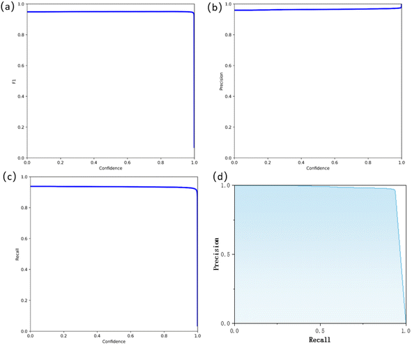
After training the Mask R-CNN28 model on 2240 microstructural images for 40![[thin space (1/6-em)]](https://www.rsc.org/images/entities/char_2009.gif) 000 epochs, it was used to identify the ferrite and austenite phases in lightweight dual-phase steel. As shown in Fig. 4a, the model achieved an outstanding F1 score of around 0.95 on the test set. The F1 score is a commonly used metric for evaluating the performance of binary classification models, providing a comprehensive reflection of the classifier's effectiveness. It ranges from 0 to 1, with values closer to 1 indicating better model performance. The F1 score effectively distinguishes between completely incorrect (0) and completely correct (1) results. With an F1 score of 0.95, the trained model demonstrates effective differentiation between the austenite (background) and ferrite phases in lightweight steel microstructures. The high F1 score not only reflects the precision of the model in detecting the target object (ferrite) but also indicates its good recognition capability for the background (austenite), effectively distinguishing between the target object and the background. This provides robust support for the subsequent analysis and characterization of lightweight dual-phase steel microstructures. Fig. 4b presents the confidence–precision curve, which shows that precision remains consistently high at around 0.94 across the entire confidence range. This indicates that the model has a strong ability to distinguish between ferrite and austenite classes. Fig. 4c illustrates the confidence–recall curve, suggesting that recall stays at a high level of 0.94 as confidence increases. This demonstrates the model's capability to comprehensively identify ferrite.
000 epochs, it was used to identify the ferrite and austenite phases in lightweight dual-phase steel. As shown in Fig. 4a, the model achieved an outstanding F1 score of around 0.95 on the test set. The F1 score is a commonly used metric for evaluating the performance of binary classification models, providing a comprehensive reflection of the classifier's effectiveness. It ranges from 0 to 1, with values closer to 1 indicating better model performance. The F1 score effectively distinguishes between completely incorrect (0) and completely correct (1) results. With an F1 score of 0.95, the trained model demonstrates effective differentiation between the austenite (background) and ferrite phases in lightweight steel microstructures. The high F1 score not only reflects the precision of the model in detecting the target object (ferrite) but also indicates its good recognition capability for the background (austenite), effectively distinguishing between the target object and the background. This provides robust support for the subsequent analysis and characterization of lightweight dual-phase steel microstructures. Fig. 4b presents the confidence–precision curve, which shows that precision remains consistently high at around 0.94 across the entire confidence range. This indicates that the model has a strong ability to distinguish between ferrite and austenite classes. Fig. 4c illustrates the confidence–recall curve, suggesting that recall stays at a high level of 0.94 as confidence increases. This demonstrates the model's capability to comprehensively identify ferrite.
The Precision–Recall (P–R) curve is an effective metric for evaluating the predictive performance of models in imbalanced classification problems. Generally, a P–R curve closer to the upper right corner indicates superior model performance. The P–R curve for a perfect classifier is a horizontal line at y = 1. The Area Under the Curve (AUC) of the P–R curve is also a metric for measuring model performance, ranging from 0 to 1, with a larger value indicating better performance. Fig. 4d displays the P–R curve of the model on the test set when the Intersection over Union (IoU) is 0.5. From the curve profile, it can be observed that it is close to the upper right corner, with an AUC of 0.95. These metrics collectively indicate that the proposed model possesses excellent generalization ability and classification quality, achieving outstanding classification accuracy in the task of austenite–ferrite classification.
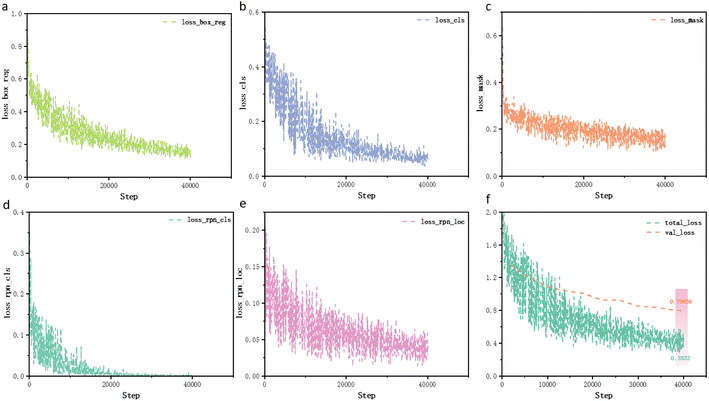
After 40![[thin space (1/6-em)]](https://www.rsc.org/images/entities/char_2009.gif) 000 iterations, the training process takes approximately only 3 hours to complete. The loss of Mask R-CNN28 consists of five components, as shown in eqn (5). loss_box_reg represents the bounding box regression loss, optimizing the model's precision in locating target objects. As depicted in Fig. 5a, the loss_box_reg value has reached approximately 0.13 and gradually stabilized after 750 epochs. loss_cls denotes the classification loss, optimizing the model's accuracy in object category classification. As shown in Fig. 5b, the loss_cls value has reached 0.06, indicating excellent classification performance. loss_mask represents the loss of the mask branch, optimizing the model's pixel-level mask prediction accuracy for target instances. As illustrated in Fig. 5c, the loss_mask value has decreased to approximately 0.12. loss_rpn_cls indicates the classification loss of the Region Proposal Network (RPN), training it to generate high-quality candidate target regions. As shown in Fig. 5d, this loss has decreased to an extremely low value of 0.001. loss_rpn_loc represents the regression loss of the RPN, optimizing the precision of locating candidate regions. As shown in Fig. 5e, the loss_rpn_loc value has decreased to approximately 0.02. The design of this multi-task loss function enables the model to simultaneously learn multiple tasks such as object detection, classification, and instance segmentation, leading to better overall performance.
000 iterations, the training process takes approximately only 3 hours to complete. The loss of Mask R-CNN28 consists of five components, as shown in eqn (5). loss_box_reg represents the bounding box regression loss, optimizing the model's precision in locating target objects. As depicted in Fig. 5a, the loss_box_reg value has reached approximately 0.13 and gradually stabilized after 750 epochs. loss_cls denotes the classification loss, optimizing the model's accuracy in object category classification. As shown in Fig. 5b, the loss_cls value has reached 0.06, indicating excellent classification performance. loss_mask represents the loss of the mask branch, optimizing the model's pixel-level mask prediction accuracy for target instances. As illustrated in Fig. 5c, the loss_mask value has decreased to approximately 0.12. loss_rpn_cls indicates the classification loss of the Region Proposal Network (RPN), training it to generate high-quality candidate target regions. As shown in Fig. 5d, this loss has decreased to an extremely low value of 0.001. loss_rpn_loc represents the regression loss of the RPN, optimizing the precision of locating candidate regions. As shown in Fig. 5e, the loss_rpn_loc value has decreased to approximately 0.02. The design of this multi-task loss function enables the model to simultaneously learn multiple tasks such as object detection, classification, and instance segmentation, leading to better overall performance.
| total_loss = loss_box_reg + loss_cls + loss_mask + loss_rpn_cls + loss_rpn_loc | (5) |
As shown in Fig. 5f, the loss function exhibits a decreasing trend, indicating a reduction in prediction errors over time. With increasing training iterations, the losses for both the training and validation sets have decreased to approximately 0.35 and 0.79, respectively, with a continuing downward trend. This indicates that the model not only demonstrates good learning capability on the training set but also exhibits strong generalization ability on new data, thereby proving that overfitting has not occurred. The sustained decrease in losses for both the training and validation sets further supports this conclusion. Conversely, it is generally believed that if the training loss continues to decrease while the validation loss gradually increases during the training process, the model may be experiencing overfitting. To address this issue, various methods can be employed, such as data augmentation, regularization, simplifying the model structure, increasing the training data, and adjusting the learning rate. These strategies collectively enhance the model's ability to generalize effectively to unseen data.
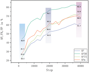
The Average Precision (AP) is a commonly used evaluation metric in computer vision tasks such as object detection and object recognition. It comprehensively measures the average precision performance of the model at different recall levels, as shown in Fig. 6. After complete training on the training set, the AP is 61.7%. At an IoU of 0.5, the AP reaches its maximum value of 82.6%; at an IoU of 0.75, the AP decreases to 72.9%, resulting in an average AP of 68.9%. Due to the presence of many small and densely distributed objects in lightweight dual-phase steel and the uneven distribution of grain sizes after annealing at 700 °C, a uniform microstructure cannot be observed. With the increase in annealing temperature, the grain size grows uniformly, leading to varying sizes of targets in the dataset. Therefore, although the AP reached 82.6% at an IoU of 0.5, the continuing upward trend effectively demonstrates that the model has not experienced overfitting and possesses good generalization ability.
In instance segmentation tasks, the accuracy of the Mask R-CNN28 model is typically assessed using multiple common metrics such as mean Average Precision (mAP), Mask Average Precision (Mask AP), pixel accuracy, and Mean Intersection over Union (Mean IoU). These metrics provide comprehensive and objective analyses of the model's detection, segmentation, and localization capabilities, serving as a basis for model optimization and deployment. In instance segmentation tasks, false negatives refer to target instances present in the ground truth but not detected or segmented by the model, while false positives indicate instances detected and segmented by the model but not present in the ground truth. Controlling the variations of these metrics is crucial for improving the accuracy and performance of instance segmentation models. As depicted in Fig. 7, the accuracy of the austenite–ferrite segmentation model has reached 0.95 and gradually stabilized after 3500 iterations, while false negatives and false positives have decreased to 0.07 and 0.06, respectively, showing a stable trend. This indicates that the model can accurately detect ferrite and precisely locate and segment it.
 | ||
| Fig. 7 Model evaluation metrics during training of the Mask R-CNN.28 Accuracy represents the model's accuracy, false_negative denotes false negatives, and false_positive denotes false positives. | ||
4.2. The detection and segmentation of austenite and ferrite phases
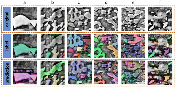
The following figure illustrates the prediction and segmentation results of lightweight dual-phase steel (i.e., austenite and ferrite) using the Mask R-CNN28 model. Fig. 10a–e depict five different microstructure images obtained from various heat treatments, randomly selected from the validation set, yet all accurately segmented as depicted in the subsequent figure results. Ferrite is masked with different colors, with bounding boxes representing detected ferrite within the test images, chosen with a reliability of 80%. The unmasked regions represent the austenite phase. The segmentation masks can differentiate ferrite of various sizes; however, some extremely small ferrite phases were not identified, possibly due to the false_negative values not meeting the expected results, as indicated by the red circle in Fig. 8.In the early stages of our research, we adopted a threshold segmentation method that is straightforward and computationally efficient. We found that threshold segmentation effectively and rapidly separates foreground from background in images with uniform lighting and high contrast. However, image noise significantly impacts the segmentation results, potentially leading to misclassifications. Furthermore, while automated thresholding methods allow for parameter adjustments, manual configuration is still necessary to accommodate different image characteristics. As illustrated in Fig. 9b, although threshold segmentation can extract a substantial portion of the ferrite structure, some regions are incorrectly identified as ferrite due to the effects of polishing and image noise. As shown in Fig. 9d, the limitations of the imaging conditions lead to the presence of dark shadow areas, where the accuracy of threshold segmentation is notably reduced in complex structures. In contrast, the Mask R-CNN28 model, as shown in Fig. 9a and c, while not achieving perfect segmentation in terms of precision, demonstrates superior performance in handling complex structures and image noise compared to the threshold segmentation method. In the early stages, we also explored commonly used object detection methods such as YOLO,27 Faster R-CNN,26 and U-Net.23 However, when constructing datasets for YOLO27 and Faster R-CNN,26 we encountered challenges due to the microstructure of the samples, which typically exhibit a reticular or plate-like pattern. In these cases, distinguishing different regions as separate entities is difficult. Additionally, both YOLO27 and Faster R-CNN26 rely on rectangular bounding boxes (represented by four parameters: x, y, w, and h, corresponding to the center coordinates and width/height of the box) during annotation using the Labelme36 tool. This approach is insufficient for capturing the complex morphology of the microstructure, thus complicating the dataset creation process. In contrast, when using U-Net23 for image segmentation, we evaluated the performance of U-Net23 and Mask R-CNN28 based on an Intersection over Union (IoU) threshold of 0.5. The results showed that U-Net23 achieved an average precision (AP) of 85.6% under this threshold, slightly outperforming Mask R-CNN.28 However, while YOLO27 and Faster R-CNN26 output bounding boxes, U-Net23 only generates segmentation masks. Mask R-CNN,28 which extends object detection with instance segmentation, is capable of producing both bounding boxes and segmentation masks. The segmentation mask allows for a more accurate measurement of grain size distribution, whereas relying solely on bounding boxes may lead to increased error.
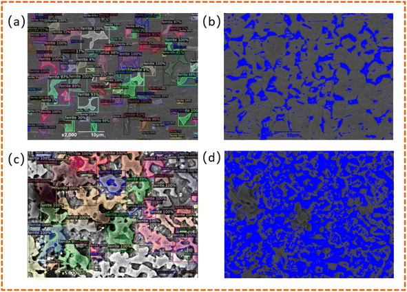 | ||
| Fig. 9 (a) and (c) show the segmentation results of Mask R-CNN,28 while (b) and (d) display the results of threshold segmentation. | ||
4.3. Statistical analysis of grain information
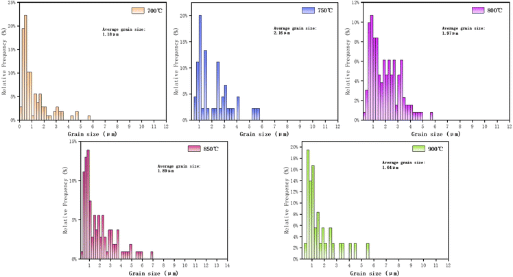
Mask R-CNN28 is a deep learning-based instance segmentation model capable of performing both object detection and semantic segmentation tasks simultaneously. It extends the well-known two-stage object detection model, Faster R-CNN,26 by adding a branch for predicting object masks. While the bounding boxes output by Faster R-CNN26 are typically regular rectangular boxes, the masks output by Mask R-CNN28 can represent irregularly shaped object regions, allowing for a better fit to the irregular shapes of ferrite and austenite structures. Using the trained model, the positions of the bounding boxes for each detected grain, the confidence scores, and the segmentation masks are output. Based on the binary masks, the pixel area of each grain instance is calculated, and the total area of all grains as a proportion of the entire image is computed as a measure of volume fraction. The equivalent diameter of the grains is calculated based on the area, and the average grain size is determined by calculating the mean diameter of all grains. In this study, a Python script was developed to extract grain information. Table 3 compares the predicted grain information from the microstructure of five different heat-treated samples with the original measured grain information. As shown in the table, the minimum prediction error for the volume fraction of ferrite and austenite is 0.1%, the maximum error is only 1.4%, and the average error is 0.9%. For the prediction of the average grain size of ferrite, the minimum error is 0.02 μm, the maximum error is 0.13 μm, and the average prediction error is 0.07 μm. For the prediction of the average grain size of austenite, the minimum error is 0.03 μm, the maximum error is 0.1 μm, and the average prediction error is 0.07 μm. It was observed that the average grain size of ferrite attains its maximum at 750 °C. This phenomenon may be attributed to the fact that, according to experimental evidence, as the heat treatment temperature increases, the average grain size of austenite continues to grow, while the average grain size of ferrite remains relatively constant. During low-temperature heat treatment, an uneven microstructure is observed, and this microstructural heterogeneity reaches a state of equilibrium at 750 °C, leading to the maximum average grain size of ferrite.| Samples | Ferrite volume fraction (%) | Average ferrite grain size (μm) | Austenite volume fraction (%) | Average austenite grain size (μm) |
|---|---|---|---|---|
| 700 °C-prediction | 45.25% | 1.18 | 54.75% | 1.61 |
| 700 °C-original | 44.46% | 1.11 | 55.54% | 1.56 |
| 750 °C-prediction | 46.13% | 2.16 | 53.87 | 1.93 |
| 750 °C-original | 44.71% | 2.03 | 55.29% | 1.90 |
| 800 °C-prediction | 38.20% | 1.97 | 61.80% | 2.00 |
| 800 °C-original | 38.87% | 1.91 | 61.13% | 1.95 |
| 850 °C-prediction | 34.42% | 1.89 | 65.58% | 3.05 |
| 850 °C-original | 34.52% | 1.83 | 65.48% | 3.01 |
| 900 °C-prediction | 33.77% | 1.64 | 66.23% | 3.16 |
| 900 °C-original | 35.13% | 1.62 | 64.87% | 3.07 |
Fig. 11 illustrates the distribution of ferrite grain sizes in lightweight dual-phase steel after heat treatment at five different temperatures. These distributions were obtained based on masks output by the Mask R-CNN28 model, whereby the equivalent diameters of each mask (i.e., ferrite grains) were computed. Overall, the segmentation capability of Mask R-CNN28 provides robust support for accurately extracting grain instance information from complex microstructure images. Through training on annotated structural data, the model can learn visual feature patterns of grains and detect and segment the precise regions of each grain on new samples, thereby enabling the computation of metrics such as volume fraction and size. This deep learning-based approach significantly outperforms traditional image processing algorithms, particularly in handling complex scenes with improved robustness and accuracy.
5. Conclusion
This study proposes a framework utilizing the Mask R-CNN deep learning model for automatic segmentation and quantification of ferrite and austenite in dual-phase steel. Initially, lightweight dual-phase steel undergoes heat treatment at five different temperatures, and the microstructure is captured using scanning electron microscopy. A dataset comprising 40 images is selected for analysis. Preprocessing techniques such as grayscale conversion and erosion are applied to reduce image noise. Subsequently, the dataset is annotated using Labelme software, and data augmentation techniques including rotation and cropping are employed. The optimal model is trained using these augmented data. The Mask R-CNN instance segmentation algorithm is then applied to obtain grain masks, followed by quantification of grain information using Python scripts. The key implementation steps of this study are as follows:(1) By relying on a small sample dataset and utilizing data preprocessing and data augmentation techniques, good segmentation results were achieved, significantly enhancing the model's performance and generalization ability, while demonstrating strong portability and wide applicability.
(2) With the allowance for transfer learning in the Mask R-CNN model, only a small-scale image dataset needs to be annotated. Training on 2240 images resulted in an F1 score of 0.95 on the ferrite and austenite datasets, indicating excellent classification performance. Losses on the training and validation sets reached around 0.35 and 0.79, respectively, suggesting good generalization of the model. The AP at IoU 0.5 reached 82.6%, demonstrating strong localization and segmentation capabilities.
(3) Mask R-CNN extends faster R-CNN by incorporating a parallel mask branch dedicated to predicting pixel-level segmentation masks for each target instance. This enables Mask R-CNN to not only detect object bounding boxes but also accurately predict object instance contours and boundaries. By obtaining contour information of each grain through masks, grain information is quantified. The average prediction error for the average grain size of ferrite and austenite is only 0.07 μm, while the prediction error for grain volume fraction is also only 0.9%.
This study achieves accurate segmentation of austenite and ferrite using the Mask R-CNN deep learning model and successfully quantifies grain information. The integration of deep learning techniques with materials science not only advances the intelligent upgrading of material analysis methods but also lays the foundation for the wider application of artificial intelligence in the field of materials, thereby contributing to the enhancement of dual-phase steel performance, promotion of intelligent manufacturing, and material genomics engineering. However, the proposed approach in this paper also has some limitations, primarily concerning the high requirements for image quality and the dependence of the model's segmentation performance on the quality of the manually annotated dataset. Additionally, there is still room for improvement in the model's average precision. To address these issues, future efforts could focus on expanding the dataset to increase sample diversity, ensuring coverage of different imaging conditions and microstructures; obtaining high-quality annotated data to enhance the training effectiveness and segmentation accuracy; and exploring improved model architectures or optimization algorithms to further enhance the model's performance and precision. Through these measures, we aim to achieve a more accurate and robust segmentation model.
Data availability
The raw data required to reproduce these findings are available to download from [https://www.scidb.cn/en/s/73eiYz]. The processed data required to reproduce these findings are available to download from [https://github.com/18811938923/F-A-Segmentation].Conflicts of interest
The authors declare that they have no known competing financial interests or personal relationships that could have appeared to influence the work reported in this paper.Acknowledgements
This work was financially supported by the Natural Science Research Foundation of China (No. 51801015). Thanks to Chengdu University, School of Mechanical Engineering.References
- H. Kim, D.-W. Suh and N. J. Kim, Fe–Al–Mn–C lightweight structural alloys: a review on the microstructures and mechanical properties, Sci. Technol. Adv. Mater., 2013, 14(1), 014205, DOI:10.1088/1468-6996/14/1/014205.
- S.-b. Bai, Y.-a. Chen, X. Liu, H.-h. Lu, P.-k. Bai, D.-z. Li, Z.-q. Huang and J.-y. Li, Research status and development prospect of Fe–Mn–C–Al system low-density steels, J. Mater. Res. Technol., 2023, 25, 1537–1559, DOI:10.1016/j.jmrt.2023.06.037.
- A. Banis, A. Gomez, V. Bliznuk, A. Dutta, I. Sabirov and R. H. Petrov, Microstructure evolution and mechanical behavior of Fe–Mn–Al–C low-density steel upon aging, Mater. Sci. Eng., A, 2023, 875, 145109, DOI:10.1016/j.msea.2023.145109.
- S. Chen, R. Rana, A. Haldar and R. K. Ray, Current state of Fe-Mn-Al-C low density steels, Prog. Mater. Sci., 2017, 89, 345–391, DOI:10.1016/j.pmatsci.2017.05.002.
- E. Wakai, H. Noto, T. Shibayama, K. Furuya, M. Ando, T. Kamada, T. Ishida and S. Makimura, Microstructures and hardness of BCC phase iron-based high entropy alloy Fe-Mn-Cr-V-Al-C, Mater. Charact., 2024, 211, 113881, DOI:10.1016/j.matchar.2024.113881.
- B. Mishra, R. Sarkar, V. Singh, D. Kumar, A. Mukhopadhyay, V. Madhu and M. J. N. V. Prasad, Effect of cold rolling and subsequent heat treatment on microstructural evolution and mechanical properties of Fe-Mn-Al-C-(Ni) based austenitic low-density steels, Mater. Sci. Eng., A, 2022, 861, 144324, DOI:10.1016/j.msea.2022.144324.
- J. Moon, S.-J. Park, C.-H. Lee, H.-U. Hong, B. H. Lee and S.-D. Kim, Influence of microstructure evolution on hot ductility behavior of austenitic Fe–Mn–Al–C lightweight steels during hot tensile deformation, Mater. Sci. Eng., A, 2023, 868, 144786, DOI:10.1016/j.msea.2023.144786.
- K.-W. Kim, S.-J. Park, J. Moon, J. H. Jang, H.-Y. Ha, T.-H. Lee, H.-U. Hong, B. H. Lee, H. N. Han, Y.-J. Lee, C.-H. Lee and S.-D. Kim, Characterization of microstructural evolution in austenitic Fe-Mn-Al-C lightweight steels with Cr content, Mater. Charact., 2020, 170, 110717, DOI:10.1016/j.matchar.2020.110717.
- J. Emo, P. Maugis and A. Perlade, Austenite growth and stability in medium Mn, medium Al Fe-C-Mn-Al steels, Comput. Mater. Sci., 2016, 125, 206–217, DOI:10.1016/j.commatsci.2016.08.041.
- T. Gupta and B. K. Ghosh, A survey of expert systems in manufacturing and process planning, Comput. Ind., 1989, 11(2), 195–204, DOI:10.1016/0166-3615(89)90106-1.
- M. L. Farinacci, M. S. Fox, I. Hulthage and M. D. Rychener, The development of aladin, an expert system for aluminum alloy design, Robotics, 1986, 2(4), 329–337, DOI:10.1016/0167-8493(86)90006-9.
- C. Xin, Y. Yin, B. Song, Z. Fan, Y. Song and F. Pan, Machine learning-accelerated discovery of novel 2D ferromagnetic materials with strong magnetization, Chip, 2023, 2(4), 100071, DOI:10.1016/j.chip.2023.100071.
- C. Xin, B. Q. Song, G. Y. Jin, Y. L. Song and F. Pan, Advancements in High-Throughput Screening and Machine Learning Design for 2D Ferromagnetism: A Comprehensive Review, Adv. Theory Simul., 2023, 6(12), 2300475, DOI:10.1002/adts.202300475.
- B. Mulewicz, G. Korpala, J. Kusiak and U. Prahl, Autonomous Interpretation of the Microstructure of Steels and Special Alloys, Mater. Sci. Forum, 2019, 949, 24–31, DOI:10.4028/www.scientific.net/MSF.949.24.
- B. L. DeCost, T. Francis and E. A. Holm, Exploring the microstructure manifold: Image texture representations applied to ultrahigh carbon steel microstructures, Acta Mater., 2017, 133, 30–40, DOI:10.1016/j.actamat.2017.05.014.
- M. Warmuzek, M. Żelawski and T. Jałocha, Application of the convolutional neural network for recognition of the metal alloys microstructure constituents based on their morphological characteristics, Comput. Mater. Sci., 2021, 199, 110722, DOI:10.1016/j.commatsci.2021.110722.
- M. Shen, G. Li, D. Wu, Y. Liu, J. R. C. Greaves, W. Hao, N. J. Krakauer, L. Krudy, J. Perez, V. Sreenivasan, B. Sanchez, O. Torres-Velázquez, W. Li, K. G. Field and D. Morgan, Multi defect detection and analysis of electron microscopy images with deep learning, Comput. Mater. Sci., 2021, 199, 110576, DOI:10.1016/j.commatsci.2021.110576.
- M. D. Zeiler and R. Fergus, Visualizing and Understanding Convolutional Networks, 2014 Search PubMed.
- S. M. Azimi, D. Britz, M. Engstler, M. Fritz and F. Mucklich, Advanced Steel Microstructural Classification by Deep Learning Methods, Sci. Rep., 2018, 8(1), 2128, DOI:10.1038/s41598-018-20037-5.
- M. R. Awan, C.-W. Chan, A. Murphy, D. Kumar, S. Goel and C. McClory, Deep Learning and Image data-based surface cracks recognition of laser nitrided Titanium alloy, Results Eng., 2024, 22, 102003, DOI:10.1016/j.rineng.2024.102003.
- K. Simonyan and A. ZissermanVery Deep Convolutional Networks for Large-Scale Image Recognition, Computer Science, arXiv, 2014, preprint, arXiv:1409.1556, DOI:10.48550/arXiv.1409.1556.
- A. R. Durmaz, M. Müller, B. Lei, A. Thomas, D. Britz, E. A. Holm, C. Eberl, F. Mücklich and P. Gumbsch, A deep learning approach for complex microstructure inference, Nat. Commun., 2021, 12(1), 6272, DOI:10.1038/s41467-021-26565-5.
- H. Zunair and A. B. Hamza, Sharp U-Net: Depthwise Convolutional Network for Biomedical Image Segmentation, Comput. Biol. Med., 2021, 136, 104699, DOI:10.1016/j.compbiomed.2021.104699.
- P. Zhao, Y. Wang, B. Jiang, M. Wei, H. Zhang and X. Cheng, A new method for classifying and segmenting material microstructure based on machine learning, Mater. Des., 2023, 227, 111775, DOI:10.1016/j.matdes.2023.111775.
- A. Baskaran, G. Kane, K. Biggs, R. Hull and D. Lewis, Adaptive characterization of microstructure dataset using a two stage machine learning approach, Comput. Mater. Sci., 2020, 177, 109593, DOI:10.1016/j.commatsci.2020.109593.
- S. Ren, K. He, R. Girshick and J. Sun, Faster R-CNN: Towards Real-Time Object Detection with Region Proposal Networks, IEEE Trans. Pattern Anal. Mach. Intell., 2017, 39(6), 1137–1149, DOI:10.1109/TPAMI.2016.2577031.
- J. Redmon, S. Divvala, R. Girshick and A. Farhadi, You Only Look Once: Unified, Real-Time Object Detection, Computer Vision & Pattern Recognition, 2016 Search PubMed.
- K. He, G. Gkioxari, P. Dollár and R. Girshick, Mask R-CNN, IEEE Trans. Pattern Anal. Mach. Intell., 2017, 42(2), 386–397, DOI:10.1109/TPAMI.2018.2844175.
- M. Ackermann, D. Iren, S. Wesselmecking, D. Shetty and U. Krupp, Automated segmentation of martensite-austenite islands in bainitic steel, Mater. Charact., 2022, 191, 112091, DOI:10.1016/j.matchar.2022.112091.
- T. Y. Lin, P. Goyal, R. Girshick, K. He and P. Dollár, Focal Loss for Dense Object Detection, IEEE Trans. Pattern Anal. Mach. Intell., 2017,(99), 2999–3007, DOI:10.48550/arXiv.1708.02002.
- C. Shen, C. Wang, M. Huang, N. Xu, S. van der Zwaag and W. Xu, A generic high-throughput microstructure classification and quantification method for regular SEM images of complex steel microstructures combining EBSD labeling and deep learning, J. Mater. Sci. Technol., 2021, 93, 191–204, DOI:10.1016/j.jmst.2021.04.009.
- D. Yang, X. Wang, H. Zhang, Z.-y. Yin, D. Su and J. Xu, A Mask R-CNN based particle identification for quantitative shape evaluation of granular materials, Powder Technol., 2021, 392, 296–305, DOI:10.1016/j.powtec.2021.07.005.
- H. Naji, L. Sancere, A. Simon, R. Büttner, M.-L. Eich, P. Lohneis and K. Bożek, HoLy-Net: Segmentation of histological images of diffuse large B-cell lymphoma, Comput. Biol. Med., 2024, 170, 107978, DOI:10.1016/j.compbiomed.2024.107978.
- M. Kalbhor, S. Shinde, P. Wajire and H. Jude, CerviCell-detector: an object detection approach for identifying the cancerous cells in pap smear images of cervical cancer, Heliyon, 2023, 9(11), e22324, DOI:10.1016/j.heliyon.2023.e22324.
- S. S. Sohn, B. J. Lee, S. Lee, N. J. Kim and J. H. Kwak, Effect of annealing temperature on microstructural modification and tensile properties in 0.35 C–3.5 Mn–5.8 Al lightweight steel, Acta Mater., 2013, 61(13), 5050–5066, DOI:10.1016/j.actamat.2013.04.038.
- K. Wada, Labelme: Image polygonal annotation with python, 2016 Search PubMed.
- G. Bradski and A. Daebler, Learning OpenCV. Computer Vision with OpenCV Library, University of Arizona Usa Since, 2008 Search PubMed.
- T. Y. Lin, M. Maire, S. Belongie, J. Hays and C. L. Zitnick, Microsoft COCO: Common Objects in Context, European Conference on Computer Vision, 2014 Search PubMed.
- S. Ren, K. He, R. Girshick and J. Sun, Faster R-CNN: Towards real-time object detection with region proposal networks, IEEE Trans. Pattern Anal. Mach. Intell., 2016, 39(6), 1137–1149 Search PubMed.
- K. He, X. Zhang, S. Ren, J. Sun, Deep Residual Learning for Image Recognition, 2016 IEEE Conference on Computer Vision and Pattern Recognition (CVPR), 2016, pp. 770–778 Search PubMed.
- T.-Y. Lin, P. Dollár, R. Girshick, K. He, B. Hariharan and S. Belongie, Feature pyramid networks for object detection, Proceedings of the IEEE Conference on Computer Vision and Pattern Recognition, 2017, pp. 2117–2125 Search PubMed.
- A. Paszke, S. Gross, F. Massa, A. Lerer, J. Bradbury, G. Chanan, T. Killeen, Z. Lin, N. Gimelshein and L. Antiga, Pytorch: An imperative style, high-performance deep learning library, Adv. Neural Inf. Process. Syst., 2019, 32, 8024–8035, DOI:10.48550/arXiv.1912.01703.
- H. Fujita, M. Itagaki, K. Ichikawa, Y. K. Hooi, K. Kawano and R. Yamamoto, Fine-tuned Pre-trained Mask R-CNN Models for Surface Object Detection, 2020 Search PubMed.
- T.-Y. Lin, M. Maire, S. Belongie, J. Hays, P. Perona, D. Ramanan, P. Dollár and C. L. Zitnick, Microsoft COCO: Common Objects in Context, in Computer Vision – ECCV 2014, ed. D. Fleet, T. Pajdla, B. Schiele and T. Tuytelaars, Springer International Publishing, Cham, 2014, pp. 740–755 Search PubMed.
- E. Hassan, N. El-Rashidy and F. M. Talaat, Review: Mask R-CNN Models, Nile J. Commun. Comput. Sci., 2022, 3(1), 280047, DOI:10.21608/njccs.2022.280047.
- Z. Xudong, Q. Lingfeng, W. Hua, Y. Hongyu, C. Zhang and H. Yanlin, In situ analysis of the deformation behavior of Fe-Mn-Al-C system lightweight steel, Shanghai Met., 2019,(2), 6, DOI:10.3969/j.issn.1001-7208.2019.02.005.
| This journal is © The Royal Society of Chemistry 2025 |

