Controlled growth of high-quality SnSe nanoplates assisted by machine learning†
Received
20th September 2024
, Accepted 17th November 2024
First published on 25th November 2024
Abstract
Machine learning (ML) approaches have emerged as powerful tools to accelerate materials discovery and optimization, offering a sustainable alternative to traditional trial-and-error methods in exploratory experiments. This study demonstrates the application of ML for controlled chemical vapor deposition (CVD) growth of SnSe nanoplates (NPs), a promising thermoelectric material. Four ML regression models are implemented to predict the side length (SL) of SnSe NPs based on CVD growth parameters. The GPR model exhibits the best performance in predicting the SL of SnSe NPs, with a coefficient of determination of 0.996, a root-mean-square error of 0.516 µm, and a mean absolute error of 0.296 µm on the test set. Then, the predicted SL of SnSe NPs is optimized through the Bayesian optimization algorithm, and the maximum SL of SnSe NPs is identified to be 32.12 µm. Validation experiments confirm the reliability of the predicted results from the constructed GPR model, with relative errors below 8% between the predicted and experimental results. These results demonstrate the robustness of ML in predicting and optimizing the CVD growth of SnSe NPs, highlighting its potential to accelerate material development and contribute to the sustainable advancement of thermoelectric materials by significantly reducing time, costs, and resource consumption associated with traditional experimental methods.
Introduction
As the focus on energy efficiency and sustainability grows, thermoelectric materials have become increasingly important in materials science because of their roles in converting waste heat into electricity. Tin selenide (SnSe) stands out in this field due to its exceptionally ultra-low lattice thermal conductivity (<0.4 W m−1 K−1 at 923 K) and high zT values (>2.3 at 723–923 K), making it a key material for sustainable energy applications.1,2 In particular, the development of two-dimensional (2D) SnSe nanoplates (NPs) has drawn significant attention, as their unique structures offer further potential for enhancing thermoelectric performance in next-generation devices.3,4 To date, SnSe NPs have been grown via different methods such as the colloid chemistry method,5 solution-phase synthesis method,4 chemical vapor deposition (CVD),6etc. Among these, CVD stands out as a facile and reliable solution for the growth of high-quality 2D SnSe NPs due to its relative simplicity and high controllability,7,8 but the lateral sizes of most reported CVD-grown SnSe NPs remain small (normally <10 µm).6,9–11
To integrate with industrial Si-based devices, the growth of large-sized SnSe NPs is essential for excellent scalability, high uniformity, and great tolerance during device fabrication, thereby reducing defects and improving consistency and yield.7 However, optimizing the CVD growth parameters to achieve the desired size of SnSe NPs is challenging due to the numerous variables involved, such as precursor temperature, temperature ramping rate, and carrier gas flow rate.7,12,13 It is difficult to figure out the ambiguous relationship between multiple growth parameters and the size of as-grown SnSe NPs. Traditional trial-and-error methods require numerous trials and have a low probability of finding the optimal parameters for large-size SnSe NPs due to the limited number of variable combinations chosen from a large parameter space. This conventional approach is not only time-consuming and resource-intensive but also environmentally unsustainable due to the excessive consumption of materials and energy.
To overcome these challenges, machine learning (ML) has emerged as an effective solution for accelerating the growth of 2D materials while promoting sustainable development in materials science. In recent years, ML has been widely applied in materials science, including new material discovery,14,15 material property prediction,16,17 and material design optimization.18 ML models are particularly beneficial because they can analyse historical experimental datasets to reveal explicit relationships between input variables and output results. This capability allows for the rapid optimization of growth parameters, minimizing the need for extensive experimental trials and thus significantly reducing resource consumption and waste. For example, some studies have proved that ML binary classification models can be used to fit the synthetic parameters of nanomaterials, thereby predicting the ‘can grow’ rate (the probability that the size of grown nanomaterials is larger than a certain size) of corresponding synthetic parameters with good prediction accuracy.19–21 In another study, Xu et al. applied an ML model to control the geometrical morphology of WTe2 nanoribbons.22 The feature importance calculated using SHapley Additive exPlanations revealed that there is a strong positive relationship between the source ratio (the molar ratio of tellurium power and tungsten power) and the length–width ratio of grown WTe2 nanostructures, enabling precise morphological control through parameter tuning. The results showed that the experimental data can be well-fitted by ML models, and the well-trained ML models help to quickly analyse and predict the experimental results.
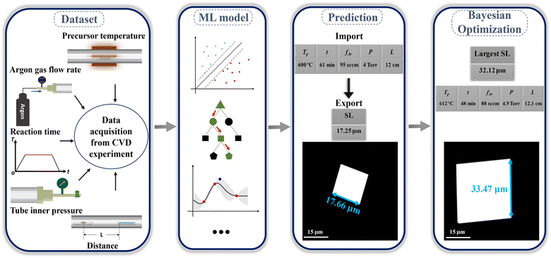
This study reports the accelerated and sustainable realization of controlled CVD growth of SnSe NPs assisted by ML, and the design framework employed for this study is depicted in Fig. 1. The data used in this work were collected from our CVD experiments. Multiple ML models were then implemented to fit the relationship between CVD growth parameters and the size of SnSe NPs. The well-trained model enabled the precise prediction of the size of SnSe NPs under random growth parameters. Based on this, the predicted side length (SL) of SnSe NPs was optimised through the Bayesian optimization algorithm, and the maximum SL and its corresponding growth parameters were subsequently identified. Several validation experiments were conducted, and the small errors between the predicted and experimental values confirmed the high reliability of the predicted results from the constructed GPR model. Overall, ML offers theoretical guidance for the controlled CVD growth of SnSe NPs and the prediction of the maximum size of SnSe NPs with minimal trials. This approach significantly impacts the controlled CVD growth of SnSe and other 2D materials, promoting the rapid and sustainable development of ML-assisted materials science, and making SnSe a more viable candidate for sustainable thermoelectric applications.
 |
| | Fig. 1 Design framework for the controlled CVD growth of SnSe NPs assisted by ML. | |
Data acquisition and variable engineering
In this paper, the CVD-grown SnSe dataset was compiled from our laboratory experiments. Fig. 2(a) shows the schematic diagram of the CVD setup for growing SnSe NPs. The detailed growth process is described in the ESI.† According to the human first–computer last strategy proposed by Kanarik et al.,23 human engineers are more proficient during the early development stages, because their experience enables better decision-making in their initial exploration. Conversely, the algorithms are far more cost-efficient in later development phases, especially when dealing with precise requirements. Therefore, integrating the specialized skills of human engineers with the efficiency of algorithms can reduce the cost-to-target compared to relying solely on either human engineers or algorithms. To minimise model computation time and optimise the fitting performance of ML models, based on the dynamic CVD growth model proposed by our group,13 the following five variables were identified by the authors as significant input variables: precursor temperature (Tp), argon gas flow rate (fAr), reaction time (t), tube inner pressure (P) and the distance between the observed sample and precursor (L). Apart from these five selected variables, other variables were considered to have negligible influence on the experimental outcomes, and they were assumed to be consistent throughout the experimental process. Given that the grown SnSe NP exhibits a square-shaped morphology, its size is appropriately quantified by measuring the SL. Thus, the output variable used in this study is the SL of the observed SnSe NPs. A total of 249 sets of data from 33 groups of experiments with different combinations of growth parameters were present in the dataset. Each set of data includes five input CVD growth parameters along with the SL of the corresponding SnSe NP. Although Tp, t, fAr, and P were kept constant within each experiment, a temperature gradient from the centre to the edges of the furnace leads to different substrates being placed at different locations along this gradient, allowing each substrate to experience a unique surface temperature. Therefore, the SnSe NPs on substrates with different L were treated as independent data points to analyse the effect of varying growth temperatures on the SL of SnSe NPs. As a result, each experiment contributed more than one set of data. Additionally, to enhance data reliability and ensure statistical robustness, multiple NPs were measured under selected growth conditions. This systematic data collection approach ensures a comprehensive and reliable dataset for our ML analysis. Table 1 shows the statistics for the input and output variables in the SnSe NP dataset, and the histogram of these variables is illustrated in Fig. 2(b). All variables follow a near-normal distribution, which is particularly beneficial for ML models as they provide balanced feature representation and facilitate effective outlier detection through standard statistical measures. This property enables the models to establish more reliable relationships between parameters while reducing the impact of extreme values.
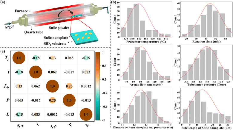 |
| | Fig. 2 (a) Schematic diagram of the CVD system used in this work; (b) histogram of input and output parameters in the statistics dataset; (c) Pearson correlation matrix heatmap among input variables. | |
Table 1 Summary of input and output variables in the statistics dataset
| Notation |
Variables |
Unit |
Min. |
Max. |
Mean |
Median |
Standard deviation |
|
T
p
|
Precursor temperature |
°C |
510 |
640 |
555.41 |
560 |
25.94 |
|
t
|
Reaction time |
min |
15 |
65 |
30.46 |
30 |
2.32 |
|
f
Ar
|
Argon gas flow rate |
sccm |
30 |
155 |
82.84 |
80 |
26.44 |
|
P
|
Tube inner pressure |
torr |
3.49 |
6.66 |
4.96 |
5 |
0.79 |
|
L
|
Distance between the observed sample and precursor |
cm |
11 |
15 |
12.58 |
12.5 |
0.81 |
| SL |
Side length of SnSe NP |
µm |
1.2 |
30.4 |
11.47 |
10.24 |
7.08 |
Fig. 2(c) illustrates the correlation analysis among input variables by calculating their Pearson correlation coefficients (PCCs).24 The PCC measures the linear relationship between any two variables, quantifying the strength and direction of the relationship. A positive value indicates the positive correlation, and vice versa; the smaller the absolute value, the lower the correlation. In our CVD experiments, the P is precisely controlled by adjusting the degree to which the downstream valve is opened, while the fAr determines the base pressure within the tube. When designing an experiment with a high P, a higher fAr is required to prevent the valve from being fully closed. Therefore, there is a certain degree of linear relationship between these two variables, with a PCC of 0.25. But overall, all PCCs between different variables are below 0.5, suggesting that these input variables are independent, which reduces the likelihood of multi-collinearity problems.25
Results and discussion
Based on the “no-free-lunch theorem”,26 no algorithm is universally superior to all others for all possible problems. Thus, in this work, four different regression models, including Gaussian process regression (GPR), support vector regression (SVR), random forest (RF), and regression tree (RT), were employed on the SnSe dataset for selecting the best model. These models have been successfully used in historical studies to address various materials science problems, especially those involving small dataset prediction.20,27–29 The detailed principles of those models are given in the ESI.† Before model training, the dataset was randomly split into a training set containing 80% of data and a test set containing 20% of data.
Hyperparameter tunning
Hyperparameters in ML models are external configurations that govern the behaviour of learning algorithms; optimizing these parameters is crucial for enhancing model performance, generalization capability, and computational efficiency. In this study, the hyperparameters for each model were tuned by using the Bayesian optimization (BO) algorithm. BO is a robust algorithm for the global optimization of objective functions based on Bayes' theorem described as eqn (1):where D and w represent the given data and unseen data, respectively; p(w|D) and p(w) represent the posterior and prior distributions, respectively; p(D|w) is the likelihood. The posterior possibility is found by integrating prior knowledge with observed data. This posterior information is then utilized to determine the location where the function achieves its extremum value.30 Compared with grid search, BO exhibits higher efficiency in high-dimensional space; at the same time, it is more reliable for training some complex models than random search.31 Therefore, BO was chosen as the optimization algorithm in this study.
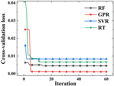
Considering the relatively small SnSe NP dataset, a 5-fold cross-validation (CV) strategy was introduced during the hyperparameter tuning process.32 The 5-fold CV guarantees that each iteration involves five repetitions of training and validation, allowing the model to be trained on a broader training set and validated across different subsets. This process helps improve model robustness, reduce the risk of overfitting, and enable effective hyperparameter search with the BO algorithm. More about the BO algorithm with a five-fold CV is given in the ESI.†Fig. 3 shows the minimum CV loss values versus iteration for different ML models during the hyperparameter tuning process. Four ML models demonstrate distinct evolution patterns in terms of CV loss values and convergence rates. Clearly, GPR and SVR take fewer iterations to converge than the other two models. Between these two, the loss value of GPR decreases sharply during the hyperparameter tuning process, which means that the BO tuned the GPR model more efficiently. But overall, four iterative curves converge within 20 iterations, indicating the reliable performance of BO in tuning hyperparameters of ML models.
 |
| | Fig. 3 Iterative curves of the minimum CV loss during the hyperparameter tuning process. | |
Performance of ML models in predicting the SL of SnSe NPs
The ML models with optimised hyperparameters were then employed to fit the SnSe NP data. To evaluate the predictive performance of each ML model, three performance parameters, such as coefficient of determination (R2), root-mean-square error (RMSE) and mean absolute error (MAE), are calculated by referring to eqn (2)–(4), respectively:29| |  | (2) |
| |  | (3) |
| |  | (4) |
where n is the number of data samples,  is the predictive value, yi is the observed value, and ȳ* and ȳ are the mean values of the predictive and observed values, respectively. R2 provides a measure of how well the ML model predicts an outcome; a higher R2 value indicates a better fit of the ML model to the data. RMSE measures the deviation between the predicted and observed values, while MAE measures the difference between the predicted and observed values. Between these two, RMSE is more sensitive to outliers, providing a measure of the typical size of prediction errors; on the other hand, MAE indicates the average prediction error magnitude without giving undue weight to outliers. A lower RMSE or MAE indicates a better fit, reflecting smaller prediction errors on average.
Fig. 4 shows the scatter plots of predicted SLs versus actual SLs of SnSe NPs on the training and test sets by using different ML models, and the corresponding R2, RMSE and MAE values are given in the lower right corner of the figures. The blue dashed line represents an ideal fit curve. Points located nearer to this line exhibit a lower variance between the predicted and observed values. For the SL prediction of SnSe NPs, SVR shows the lowest performance with an R2 value of 0.894, which can be attributed to its fundamental working mechanism. In our dataset, samples in the large SL region (>20 µm) are relatively sparse, leading to insufficient support vectors.33 This limitation makes it challenging for the SVR model to establish accurate decision boundaries, resulting in less stable predictions. In contrast, GPR, RT, and RF models demonstrate superior performance with higher R2 values on the test set (0.996, 0.943, and 0.964, respectively), indicating their better capability in capturing the complex relationships between CVD growth parameters and the SL of SnSe NPs. Among these three models, GPR has the lowest RMSE and MAE values (0.516/0.296 µm) on the test set compared with those of RT (1.981/1.4 µm) and RF (1.561/1.304 µm), indicating the low prediction error of the GPR model. In addition, the R2, RMSE and MAE values of the GPR model on the training set and test set are very close, indicating that the overfitting issue did not occur. Therefore, the GPR model is recommended as the most suitable model for predicting the SL of SnSe NPs. It should be noteworthy that although GPR performs slightly better in predicting the SL of SnSe NPs, RT and RF are also efficient models with good prediction accuracy. The performance statistics of different models are summarized in Table S1.†
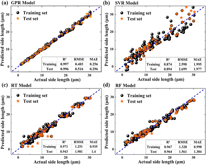 |
| | Fig. 4 Scatter plot of predicted versus actual values using different ML models: (a) GPR model; (b) SVR model; (c) RT model; and (d) RF model. | |
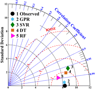
The predictive performance of each model can also be graphically indicated by a Taylor diagram.34 The Taylor diagram shown in Fig. 5 describes the relationship between the real observed value and the predictive value of each ML model by referring to the integration of standard deviation (SD), RMSE, and the correlation coefficient value in a polar coordinate. It can be seen that the GPR model is situated nearest to the observed point for SnSe NP SL prediction, exhibiting the highest correlation coefficient, the lowest RMSE and a SD that most closely matches the observed point. This suggests that the GPR model has the best predictive ability among the four models. Fig. S6† shows the estimated error distributions between the predicted SLs and actual SnSe NP SLs based on different ML models. For all ML models, it is evident that the errors are symmetrically distributed around zero, showing the effective performance of the four models. Among them, the error distribution of the GPR model has a narrower spread, further verifying that the GPR model has the highest prediction accuracy.
 |
| | Fig. 5 Taylor diagram of different ML models for SnSe SL prediction. | |
CVD growth parameter optimization for the maximum SL of SnSe NPs
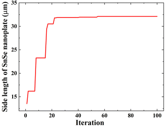
The predictive performance discussed above proved that the experimental data can be well-fitted by the GPR model. Next, by setting the predictive SL from the trained GPR model as the objective function, the BO algorithm was employed again to find out the maximum value of the SL of SnSe NPs and the corresponding CVD growth parameters. To make sure that the input variables vary in a reasonable range through the optimization process, the range constraint for solving this optimization problem is defined as eqn (5):where Di is the ith input variable, and Dimin and Dimax are the lower and upper limit values of the variable given in Table 1, respectively. The process of BO is shown in Fig. 6. The predicted maximum SL of SnSe NPs increases during the first several iterations and stabilized after 55 iterations, indicating that the global optimum is found. Ultimately, the maximum SL identified by the BO is confirmed to be 32.12 µm, with the corresponding optimal growth parameters being: Tp of 612 °C, t of 48.1 min, fAr of 87.8 sccm, P of 4.9 torr, and L of 12.1 cm.
 |
| | Fig. 6 Observed maximum SL of SnSe NPs versus iteration through the BO algorithm. | |
As recorded in Table 1, the maximum SL of the grown SnSe NPs from our dataset is 30.4 µm, which is smaller than the predicted maximum SL by the BO algorithm. But it should be noted that the difference between these two values is not significant, suggesting the experimental growth parameters for achieving a SL of 30.4 µm are close to the optimal ones. This also indicates that the theoretical optimal growth parameters were missed out in the previous limited experiments. Finding the exact optimal conditions by continuously adjusting experimental parameters would require a considerable amount of time and resources. In contrast, with the assistance of the BO algorithm, the theoretical maximum value can be quickly identified along with its corresponding growth condition. This approach significantly improves the efficiency of the CVD growth optimization and shortens the development cycle.
Building upon this, while the current study utilizes GPR and BO to optimize the CVD growth parameters for SnSe NPs, future investigations could further benefit from incorporating the multi-fidelity Gaussian process (MF-GP) model. The MF-GP model offers the advantage of combining both low-fidelity and high-fidelity datasets, where low-fidelity data can provide quick insights and high-fidelity data ensure precision in predictions. Recent studies have shown that the MF-GP model not only accelerates the optimization process by reducing the reliance on high-cost, high-fidelity data, but also maintains or even enhances prediction accuracy in high-dimensional parameter spaces.35,36 By integrating the MF-GP model, future studies may achieve even greater computational efficiency, particularly in high-cost experimental or simulation settings, thus enabling faster convergence and more accurate predictions.
Variable importance analysis
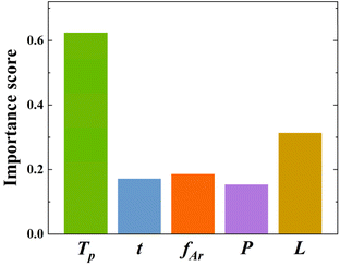
To gain a clear understanding of the CVD growth of SnSe NPs, a global sensitivity analysis (SA) was applied to extract the variable importance scores for the SL prediction of SnSe NPs. SA is based on the principle of variance decomposition, assessing the contribution of input variables and their interactions to the output variance of the model, thereby identifying the variable importance scores.37 From Fig. 7, it is evident that Tp is the most sensitive variable affecting the SL of SnSe NPs with an importance score of 0.62, which agrees well with many experimental findings from previous studies that Tp influences the size of CVD-grown nanomaterials significantly.13,38 The relationship between the total vapour pressure of solid SnSe and Tp can be described with eqn (6):| |  | (6) |
where Ps is the vapour pressure of solid SnSe at Tp.6 Obviously, Ps increase with Tp, which determines the amount of vaporized SnSe molecules delivered onto the substrate surface for growing NPs, thereby modulating NP growth. L also has a significant influence on the SL of SnSe NPs with an importance score of 0.31. When Tp is fixed, L directly determines the growth temperature (Tg) of the observed sample. By referring to eqn (7):| |  | (7) |
where Ks is the reaction constant on the substrate surface, k is the Boltzmann constant, and Ea is the apparent activation energy of the growth.13Ks is proportional to Tg and in turn controls the growth rate of NPs and ultimately the SL of the NPs.39 While less influential, other parameters also play roles in SnSe NP growth. t, fAr, and P have similar influences on the SL of SnSe NPs with importance scores of 0.17, 0.18 and 0.15, respectively. Consequently, selecting appropriate growth parameters is important for the SL of SnSe NPs, from both an ML and an experimental perspective. This analysis can serve as general guidance for the CVD growth of SnSe NPs and potentially other nanomaterials in future experimental work, enabling more precise control over nanostructure dimensions.
 |
| | Fig. 7 Variable importance scores using SA. | |
Model validation
To further verify the reliability of the constructed GPR model, several experiments were conducted in which the growth parameters had not been used for model training. The model was validated by calculating the relative error between the measured SLs of SnSe NPs from experiments and the predicted SLs from the ML model, as shown in Table 2. Notably, the growth parameters for the 1st sample are found to be the optimal growth parameters by the BO algorithm with a predicted maximum SL of 32.12 µm. Notably, this achieved SL of SnSe NPs surpasses the SLs reported in numerous previous studies.6,9–11,40Fig. 8(a) displays the SEM image of the SnSe NPs prepared under these conditions, with a measured SL of 33.47 µm. The relative error between the experimental and predicted values is 4.03%, which demonstrates the feasibility of the predicted maximum SL from the ML model. The relative errors for the remaining samples are 1.06%, 3.86%, 7.31%, 2.32% and 3.13%, respectively. The SEM images of the grown SnSe NPs under these conditions are shown in Fig. 8(b)–(f). In summary, all relative errors in the experimental validation test do not exceed 8%, indicating the high reliability of the predicted results from the constructed GPR model. These results prove that the trained ML model can facilitate the CVD growth of SnSe NPs with larger sizes.
Table 2 Model validation table
| Sample |
T
p (°C) |
t (min) |
f
Ar (sccm) |
P (torr) |
L (cm) |
Predicted SL from ML (µm) |
Measured SL from experiment (µm) |
Relative error (%) |
|
1
|
612
|
48
|
88
|
4.9
|
12.1
|
32.12
|
33.47
|
4.03
|
| 2 |
630 |
35 |
55 |
5 |
12 |
27.56 |
27.27 |
1.06 |
| 3 |
535 |
55 |
65 |
4 |
12.5 |
9.68 |
9.32 |
3.86 |
| 4 |
550 |
60 |
38 |
3.4 |
12 |
11.79 |
12.72 |
7.31 |
| 5 |
600 |
61 |
95 |
4 |
12 |
17.25 |
17.66 |
2.32 |
| 6 |
525 |
35 |
75 |
5 |
13.5 |
3.95 |
3.83 |
3.13 |
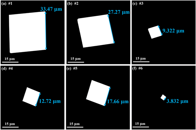 |
| | Fig. 8 Representative SEM images of (a) sample #1; (b) sample #2; (c) sample #3; (d) sample #4; (e) sample #5; and (f) sample #6. | |
Material characterization
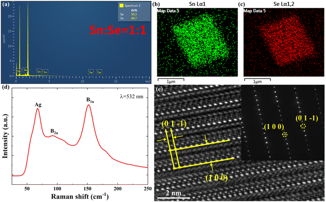
Finally, to evaluate the physical properties of grown SnSe NPs, several characterization techniques were carried out. The energy-dispersive X-ray spectroscopy (EDS) spectrum in Fig. 9(a) confirms the presence of Sn and Se elements in the NP, and the chemical composition ratio of Sn to Se is identified to be approximately 1![[thin space (1/6-em)]](https://www.rsc.org/images/entities/char_2009.gif) :
:![[thin space (1/6-em)]](https://www.rsc.org/images/entities/char_2009.gif) 1, which is consistent with the expected chemical stoichiometry ratio within experimental error. Fig. 9(b) and (c) depict the EDS mapping of a representative SnSe NP, demonstrating uniform distributions of Sn and Se elements across the NP. The Raman spectrum of a representative SnSe NP was also recorded via Raman spectroscopy under 532 nm laser illumination at room temperature. As shown in Fig. 9(d), three characteristic peaks at 67 cm−1, 92 cm−1 and 152 cm−1 are observed, which correspond to the Ag. B2u and B1u modes of SnSe, respectively.6,41 The recorded Raman spectrum is consistent with those reported previously, confirming the formation of pure SnSe NPs.
1, which is consistent with the expected chemical stoichiometry ratio within experimental error. Fig. 9(b) and (c) depict the EDS mapping of a representative SnSe NP, demonstrating uniform distributions of Sn and Se elements across the NP. The Raman spectrum of a representative SnSe NP was also recorded via Raman spectroscopy under 532 nm laser illumination at room temperature. As shown in Fig. 9(d), three characteristic peaks at 67 cm−1, 92 cm−1 and 152 cm−1 are observed, which correspond to the Ag. B2u and B1u modes of SnSe, respectively.6,41 The recorded Raman spectrum is consistent with those reported previously, confirming the formation of pure SnSe NPs.
 |
| | Fig. 9 (a) EDS spectrum; (b) and (c) EDS mappings; (d) Raman spectrum; (e) HRTEM image and its corresponding SAED pattern of a representative CVD-grown SnSe NP. | |
For a more detailed investigation into the crystallographic properties, transmission electron microscopy (TEM) analysis was performed on the grown SnSe NP. A high-resolution TEM (HRTEM) image of a typical SnSe NP is shown in Fig. 9(e), revealing that the well-resolved crystal planes, namely (1 0 0) and (0 1 −1), are stacked with a periodic atomic arrangement, displaying interplanar spacings of 1.13 nm and 0.3 nm, respectively. These spacings are consistent with those reported in previous studies for SnSe crystals in the Pnma space group.6,42 Additionally, the inset of Fig. 9(e) shows a selective area electron diffraction (SAED) pattern obtained from the HRTEM analysis, where the distinct diffraction spots with five-fold symmetry indicate the single-crystalline nature of the SnSe NP, confirming its excellent crystal quality. The indexed crystal planes (1 0 0) and (0 1 −1) align with the SnSe planes of ICSD card # 12863, further confirming the orthorhombic crystal structure of the SnSe NP shown in the HRTEM image.
Conclusions
In this work, ML was successfully applied to fit an experimental database, enabling precise SL prediction of SnSe NPs under random growth parameters and the rapid identification of optimal growth parameters for growing the largest SnSe NPs. Four ML regression models were utilized for the SL prediction of SnSe NPs. Among them, the GPR model exhibited the best performance in predicting the SL of SnSe NPs, with a R2 of 0.996, a RMSE of 0.516 µm and a MAE of 0.296 µm on the test set. Then, the predicted SL of SnSe NPs from the well-trained GPR model was optimised through the BO algorithm, and the theoretical maximum SL of SnSe NPs was found to be 32.12 µm, with the corresponding optimal growth parameters being: Tp of 612 °C, t of 48.1 min, fAr of 87.8 sccm, P of 4.9 torr and L of 12.1 cm. The calculated variable importance showed that Tp was the most crucial parameter for the CVD growth of SnSe NPs. Finally, several validation experiments were conducted, and all the relative errors between the experimental results and predicted results were less than 8%, indicating the high reliability of the predicted results from the constructed GPR model. Additional characterization results confirmed the correct chemical stoichiometry and high crystal quality of the as-grown SnSe NPs. In summary, this study goes beyond the use of ML in simulations or online datasets, demonstrating its direct impact on actual experimental workflows. ML not only provides theoretical support for guiding the controlled CVD growth of SnSe NPs but also offers a sustainable approach by significantly reducing the number of experimental trials required to achieve optimal results. This reduction in experimental iterations translates to lower resource consumption, energy usage, and waste generation, thereby contributing to a more environmentally responsible material growth process. The integration of ML analysis with experimental validations demonstrates the substantial potential of ML in accelerating the growth of 2D materials and advancing the field of ML-assisted materials science in a sustainable manner.
Data availability
The data that support this study are available from the corresponding author upon reasonable request.
Author contributions
H. J. Luo: conceptualization, software, investigation, data curation, visualization, validation, and writing – original draft; W. W. Pan: software, investigation, and writing – review & editing; J. L. Liu: conceptualization and methodology; H. Wang: data curation and formal analysis; S. Q. Zhang: visualization; Y. L. Ren: writing – review & editing; C. L. Yuan: writing – review & editing; W. Lei: resources, supervision, and writing – review & editing.
Conflicts of interest
There are no conflicts to declare.
Acknowledgements
The authors would like to express their sincere gratitude for the assistance provided by the Australian Research Council (LP230201028, LE230100019, CE200100010, DP200103188, and LE200100032) and the Centre for Microscopy, Characterization and Analysis (CMCA) at the University of Western Australia.
Notes and references
- L. D. Zhao, S. H. Lo, Y. S. Zhang, H. Sun, G. J. Tan, C. Uher, C. Wolverton, V. P. Dravid and M. G. Kanatzidis, Nature, 2014, 508, 373–377 CrossRef CAS.
- J. P. Heremans, Nature, 2014, 508, 327–328 CrossRef CAS PubMed.
- S. Li, Y. X. Hou, D. Li, B. Zou, Q. T. Zhang, Y. Cao and G. D. Tang, J. Mater. Chem. A, 2022, 10, 12429–12437 RSC.
- S. Chandra, P. Dutta and K. Biswas, ACS Nano, 2022, 16, 7–14 CrossRef CAS.
- W. Wang, P. H. Li, H. Zheng, Q. Liu, F. Lv, J. D. Wu, H. Wang and S. J. Guo, Small, 2017, 13, 1702228 CrossRef.
- H. Wang, S. Q. Zhang, T. Z. Zhang, J. L. Liu, Z. K. Zhang, G. Yuan, Y. J. Liang, J. Tan, Y. L. Ren and W. Lei, ACS Appl. Nano Mater., 2021, 4, 13071–13078 CrossRef CAS.
- P.-C. Shen, Y. Lin, H. Wang, J.-H. Park, W. S. Leong, A.-Y. Lu, T. Palacios and J. Kong, IEEE Trans. Electron Devices, 2018, 65, 4040–4052 CAS.
- H. Wang, R. R. Liu, S. Q. Zhang, Y. J. Wang, H. J. Luo, X. Sun, Y. L. Ren and W. Lei, Opt. Mater., 2022, 134, 113174 CrossRef CAS.
- T. F. Pei, L. H. Bao, R. S. Ma, S. R. Song, B. H. Ge, L. M. Wu, Z. Zhou, G. C. Wang, H. F. Yang, J. J. Li, C. Z. Gu, C. M. Shen, S. X. Du and H. J. Gao, Adv. Electron. Mater., 2016, 2, 1600292 CrossRef.
- F. Yang, M.-C. Wong, J. Mao, Z. Wu and J. Hao, Nano Res., 2023, 16, 11839–11845 CrossRef CAS.
- S. Zhao, H. Wang, Y. Zhou, L. Liao, Y. Jiang, X. Yang, G. Chen, M. Lin, Y. Wang and H. Peng, Nano Res., 2015, 8, 288–295 CrossRef CAS.
- J. L. Liu, H. Wang, X. Li, H. Chen, Z. K. Zhang, W. W. Pan, G. Q. Luo, C. L. Yuan, Y. L. Ren and W. Lei, J. Alloys Compd., 2019, 798, 656–664 CrossRef CAS.
- W. Lei, I. Madni, Y. L. Ren, C. L. Yuan, G. Q. Luo and L. Faraone, Appl. Phys. Lett., 2016, 109, 083106 CrossRef.
- M. Zhong, K. Tran, Y. Min, C. Wang, Z. Wang, C.-T. Dinh, P. De Luna, Z. Yu, A. S. Rasouli, P. Brodersen, S. Sun, O. Voznyy, C.-S. Tan, M. Askerka, F. Che, M. Liu, A. Seifitokaldani, Y. Pang, S.-C. Lo, A. Ip, Z. Ulissi and E. H. Sargent, Nature, 2020, 581, 178–183 CrossRef CAS.
- S. Lu, Q. Zhou, Y. Guo and J. Wang, Chem, 2022, 8, 769–783 CAS.
- A. Rodriguez, S. Lam and M. Hu, ACS Appl. Mater. Interfaces, 2021, 13, 55367–55379 CrossRef CAS.
- T. Yamashita, N. Sato, H. Kino, T. Miyake, K. Tsuda and T. Oguchi, Phys. Rev. Mater., 2018, 2, 013803 CrossRef.
- K. Guo, Z. Yang, C.-H. Yu and M. J. Buehler, Mater. Horiz., 2021, 8, 1153–1172 RSC.
- M. Lu, H. Ji, Y. Zhao, Y. Chen, J. Tao, Y. Ou, Y. Wang, Y. Huang, J. Wang and G. Hao, ACS Appl. Mater. Interfaces, 2022, 15, 1871–1878 CrossRef.
- Y. X. Chen, H. N. Ji, M. Y. Lu, B. Liu, Y. Zhao, Y. Y. Ou, Y. Wang, J. D. Tao, T. Zou, Y. Huang and J. L. Wang, Ceram. Int., 2023, 49, 30794–30800 CrossRef CAS.
- B. J. Tang, Y. H. Lu, J. D. Zhou, T. Chouhan, H. Wang, P. Golani, M. Z. Xu, Q. Xu, C. T. Guan and Z. Liu, Mater. Today, 2020, 41, 72–80 CrossRef CAS.
- M. Z. Xu, B. J. Tang, Y. H. Lu, C. Zhu, Q. B. Lu, L. Zheng, J. Y. Zhang, N. N. Han, W. D. Fang, Y. X. Guo, J. Di, P. Song, Y. M. He, L. X. Kang, Z. Y. Zhang, W. Zhao, C. T. Guan, X. W. Wang and Z. Liu, J. Am. Chem. Soc., 2021, 143, 18103–18113 CrossRef CAS PubMed.
- K. J. Kanarik, W. T. Osowiecki, Y. Lu, D. Talukder, N. Roschewsky, S. N. Park, M. Kamon, D. M. Fried and R. A. Gottscho, Nature, 2023, 616, 707–711 CrossRef CAS PubMed.
-
I. Cohen, Y. Huang, J. Chen, J. Benesty, J. Benesty, J. Chen, Y. Huang and I. Cohen, Noise Reduction in Speech Processing, 2009, pp. 1–4 Search PubMed.
- C. F. Dormann, J. Elith, S. Bacher, C. Buchmann, G. Carl, G. Carré, J. R. G. Marquéz, B. Gruber, B. Lafourcade, P. J. Leitao, T. Münkemüller, C. McClean, P. E. Osborne, B. Reineking, B. Schröder, A. K. Skidmore, D. Zurell and S. Lautenbach, Ecography, 2013, 36, 27–46 CrossRef.
- D. H. Wolpert and W. G. Macready, IEEE Trans. Evol. Comput., 1997, 1, 67–82 CrossRef.
- N. Yoshihara, Y. Tahara and M. Noda, Asia-Pac. J. Chem. Eng., 2023, 18, 2911 CrossRef.
- J. T. Wang, M. Y. Lu, Y. X. Chen, G. L. Hao, B. Liu, P. H. Tang, L. Yu, L. Wen and H. N. Ji, Nanomaterials, 2023, 13, 2283 CrossRef CAS.
- J. Zhang, Y. Huang, Y. Wang and G. Ma, Constr. Build. Mater., 2020, 253, 119208 CrossRef.
-
J. Snoek, H. Larochelle and R. P. Adams, arXiv, 2012, preprint, arXiv:1206.2944, DOI:10.48550/arXiv.1206.2944.
- J. Wu, X.-Y. Chen, H. Zhang, L.-D. Xiong, H. Lei and S.-H. Deng, J. Electron. Sci. Technol., 2019, 17, 26–40 Search PubMed.
- G. C. Cawley and N. L. C. Talbot, J. Mach. Learn. Res., 2010, 11, 2079–2107 Search PubMed.
- A. J. Smola and B. Schölkopf, Stat. Comput., 2004, 14, 199–222 CrossRef.
- K. E. Taylor, J. Geophys. Res.: Atmos., 2001, 106, 7183–7192 CrossRef.
- M. F. Lazin, C. R. Shelton, S. N. Sandhofer and B. M. Wong, Mach. Learn.: Sci. Technol., 2023, 4, 045014 Search PubMed.
-
K. Ravi, V. Fediukov, F. Dietrich, T. Neckel, F. Buse, M. Bergmann and H.-J. Bungartz, arXiv, 2024, preprint, arXiv:2404.11965, DOI:10.48550/arXiv.2404.11965.
- S. R. Arwade, M. Moradi and A. Louhghalam, Eng. Struct., 2010, 32, 1–10 CrossRef.
- S. Zhang, H. Luo, H. Wang, J. Liu, A. Suvorova, Y. Ren, C. Yuan and W. Lei, Opt. Mater., 2024, 150, 115220 CrossRef CAS.
- H. Luo, H. Wang, S. Zhang, J. Liu, Y. Ren, C. Yuan and W. Lei, J. Alloys Compd., 2024, 1008, 176819 CrossRef CAS.
- L. Qiu, X. F. Lai and J. K. Jian, Mater. Charact., 2021, 172, 110864 CrossRef CAS.
- H. R. Chandrasekhar, R. G. Humphreys, U. Zwick and M. Cardona, Phys. Rev. B: Solid State, 1977, 15, 2177 CrossRef CAS.
- P. Wu, Y. Ishikawa, M. Hagihala, S. Lee, K. L. Peng, G. Y. Wang, S. Torii and T. Kamiyama, Physica B Condens. Matter, 2018, 551, 64–68 CrossRef CAS.
|
| This journal is © The Royal Society of Chemistry 2025 |
Click here to see how this site uses Cookies. View our privacy policy here.  c and
Wen
Lei
 *a
*a


 is the predictive value, yi is the observed value, and ȳ* and ȳ are the mean values of the predictive and observed values, respectively. R2 provides a measure of how well the ML model predicts an outcome; a higher R2 value indicates a better fit of the ML model to the data. RMSE measures the deviation between the predicted and observed values, while MAE measures the difference between the predicted and observed values. Between these two, RMSE is more sensitive to outliers, providing a measure of the typical size of prediction errors; on the other hand, MAE indicates the average prediction error magnitude without giving undue weight to outliers. A lower RMSE or MAE indicates a better fit, reflecting smaller prediction errors on average.


![[thin space (1/6-em)]](https://www.rsc.org/images/entities/char_2009.gif) :
:![[thin space (1/6-em)]](https://www.rsc.org/images/entities/char_2009.gif) 1, which is consistent with the expected chemical stoichiometry ratio within experimental error. Fig. 9(b) and (c) depict the EDS mapping of a representative SnSe NP, demonstrating uniform distributions of Sn and Se elements across the NP. The Raman spectrum of a representative SnSe NP was also recorded via Raman spectroscopy under 532 nm laser illumination at room temperature. As shown in Fig. 9(d), three characteristic peaks at 67 cm−1, 92 cm−1 and 152 cm−1 are observed, which correspond to the Ag. B2u and B1u modes of SnSe, respectively.6,41 The recorded Raman spectrum is consistent with those reported previously, confirming the formation of pure SnSe NPs.
1, which is consistent with the expected chemical stoichiometry ratio within experimental error. Fig. 9(b) and (c) depict the EDS mapping of a representative SnSe NP, demonstrating uniform distributions of Sn and Se elements across the NP. The Raman spectrum of a representative SnSe NP was also recorded via Raman spectroscopy under 532 nm laser illumination at room temperature. As shown in Fig. 9(d), three characteristic peaks at 67 cm−1, 92 cm−1 and 152 cm−1 are observed, which correspond to the Ag. B2u and B1u modes of SnSe, respectively.6,41 The recorded Raman spectrum is consistent with those reported previously, confirming the formation of pure SnSe NPs.
