A density functional theory study of dye-sensitized solar cells with graphene quantum dots: only a matter of size?

Abstract

In this work, we investigate the electronic interaction between graphene quantum dots (GQDs) of varying sizes, organic dye sensitizers and a TiO₂-cluster. The dyes included here have been previously investigated by means of density functional theory in models for dye-sensitized solar cells (DSSCs). It was shown that local hybrid functionals are highly suitable for the calculation of spectra and level alignments at the dye-semiconductor interface. Here, their assessment is extended to GQDs and their combination with dyes and TiO₂-clusters. The focus of this work lies in understanding the electron-transfer mechanism of GQD implementation in a typical DSSC. Our systematic approach includes investigating individual GQDs, their compatibility with dyes and a semiconductor (TiO₂) and at the end, the more complex system dye@GQD@TiO₂. The overall charge transfer mechanism depends crucially on the graphene sheet sizes, and the dyes can have versatile roles. That is, even without direct participation in the charge injection, they are vital for light absorption and exciton generation and thus facilitate charge injection into the semiconductor.

---

1. Introduction

The experimental synthesis of a graphene monolayer sheet in 2004 opened the door for many opportunities in materials science, which ultimately led to the Nobel Prize in 2010.¹ From this point on, careful and systematic studies of various graphitic forms and properties have been conducted continuously. Structural modifications of graphene led to the discovery of graphene quantum dots (GQDs) with promising properties, such as tunable band-gaps, thermal stability and catalytic activity.^2–8 Consequently, GQDs have been introduced as an additional component in dye sensitized solar cells (DSSCs) to enhance the light harvesting efficiency (LHE) of photosensitizers.^9,10 Due to their particular electrical and optical properties in addition to large charge mobilities, GQDs can extend the absorption spectrum of the existing dyes, facilitate faster electron transfer and reduce recombination losses.^5,11,12

Recent investigations have shown that the exciton lifetime is improved through the usage of GQDs in combination with TiO₂ as a semiconductor, where the GQD takes on the role of an electron acceptor and transmitter.¹³ The energy levels between the conduction band of TiO₂ and the work function of the transparent conductive oxide (TCO), such as fluorine-doped tin oxide (FTO) are perfectly aligned.

On top of that, in GQDs there is a phenomenon called multiple exciton generation (MEG) which corresponds to the excitation of multiple electrons upon absorption of a single photon.¹⁴ In contrast, conventional bulk semiconductors feature a one-to-one correspondence between the number of incident photons and generated electrons. The size of a GQD has a significant influence on its optical properties, and recent studies showed that increasing the concentration of the sample will enhance light absorption as a crucial factor for DSSC performance.¹³ In addition, doping the basal plane and edges can substantially change the surface chemistry and electronic properties.^15–19 Introducing graphene monolayers into TiO₂ nanoparticles facilitates the rapid migration of photogenerated electrons through the photoanode.²⁰ If a single layer of GQDs is inserted between the dye and the TiO₂ nanoparticles, the charge transfer mechanism appears to change and the GQDs assist in charge separation after photon absorption.²¹ In contrast to such a layer-by-layer assembly, it has also been shown experimentally that improved photon-to-current characteristics are obtained by immersing TiO₂ nanoparticles in dye–GQD mixtures.²² Intermediate treatment of TiO₂ nanoparticles with TiCl₄ increases the surface for the adsorption of dye–GQD mixtures, resulting in significantly higher short-circuit currents.²³

Computational models using density functional theory (DFT) and linear-response time-dependent DFT (TD-TDFT) provide valuable insight into the charge-transfer mechanism at the interface of photosensitizers and a semiconductor. However, it has been shown that the choice of the method, i.e. the exchange–correlation functional influences the electronic structure at the interface significantly.^24,25 In a recent study¹⁶ the electronic coupling between a GQD (C54H18) and several small anthoxanthin dyes has been investigated using the global hybrid functional B3LYP. It revealed improved optical properties of GQD–dye nanocomposites as compared to the isolated dyes but suggests that the excited photon is localized at the GQD, which would probably lead to undesirably fast charge recombination.

In another DFT study²⁶ employing the B3LYP functional for structures and the range-separated hybrid CAM-B3LYP for excited states, the photoelectric performance of three different dyes with a D–A′–π–A structure (D = donor, A = acceptor, and π = bridge) with and without a GQD (C54H18) has been investigated. It shows a slight increase in the light-harvesting efficiency (LHE) of the dye@GQD systems as compared to the isolated dyes, but the absorption maximum of the nanocomposites is somewhat blue-shifted. Although the authors claim that adding GQDs leads to higher short-circuit current densities and open-circuit voltages, this statement is mostly based on more efficient regeneration which is customarily estimated from the HOMO energy of the isolated photosensitizers. In the same study a small TiO₂ cluster with about ten Titanium atoms was used to represent a combined dye@GQD@TiO₂ system, where the dye was directly linked to the TiO₂. However, it has been shown previously that CAM-B3LYP yields erroneous level alignments in dye@TiO₂ systems with a sizable TiO₂-cluster.

Although the aforementioned studies revealed an interesting charge-transfer mechanism through the combination of organic dyes with GQDs hinting at potentially higher power conversion efficiencies in DSSCs, a systematic and comprehensive study with varying GQD sizes and chemically diverse dyes and a careful examination of the theoretical method are still missing. Thus, this work investigates computational models of pristine GQDs introduced into previously examined dye@TiO₂ systems with structurally distinct dyes^25,27 that have been shown to be efficient sensitizers. For the nanocomposites, three sizes of GQDs are considered along with three dyes: a simple push–pull, a fully conjugated push–pull and a double donor dye (see 1). We examine the optical properties and charge distributions of the GQDs and GQD–dye nanocomposites, as well as the level alignments at the interface to a sizable TiO₂-cluster. To assess the influence of the exchange–correlation functional, DFT and TD-DFT calculations are performed with three different types of exchange–correlation functionals: global, range-separated and local hybrid functionals.^28–30

2. Models and computational details

All calculations were performed with the TURBOMOLE program suite for the quantum-chemical simulations.³¹ The structures in this work were built and visualized with VESTA and Avogadro, optimized with the B3LYP exchange–correlation functional and 6-31G* basis set.^28,32–35 The conductor-like screening model (COSMO) is used in all calculations with standard settings for water as a solvent.³⁶ Water is used since GQDs showed high solubility and experimental values in water are available to validate our results. Also, DSSCs are often combined with water-based electrolytes. An accurate representation of the semiconductor nanoparticles is established through the (TiO₂)₃₈ anatase cluster used in previous studies.^{24,25,27,37,38} Three different sizes of the GQDs were used (C42, C54 and C66) together with already examined dyes in our group (WD8, D102 and JK2) (the B3LYP/6-31G* optimized structures are shown in Fig. 1). For the excited state calculations we also used the range-separated functional CAM-B3LYP and the local hybrid functional Lh12ct-SsifPW92.^29,39–41

Fig. 1 Optimized structures at the B3LYP/6-31G*-level of three different GQDs and the three investigated dyes (WD8, D102 and JK2). C atoms (brown), H atoms (white), O atoms (red), S atoms (yellow), and N atoms (blue).

3. Theory

Since we are comparing two established exchange–correlation functionals to a local hybrid functional, that has only recently been applied to dye–semiconductor interfaces, we provide a brief summary of the different exchange–correlation functionals used in this work.

The emergence of global hybrid functionals introduced by Becke²⁸ has boosted the application of DFT in molecular and materials modelling. By adding a constant fraction of the exact-exchange energy (from the Hartree–Fock approximation), it is possible to obtain accurate band gaps as well as basic chemical properties. The general formulation of a simple global hybrid exchange functional is as follows:

E^GH_x = a₀E^ex_x + (1 − a₀)E^sl_x (1)

where E^sl_x is a semi-local approximation and E^ex_x is the exact exchange energy, combined with some fixed amount, a₀. The fraction a₀ is a fixed and system-wide parameter. With global hybrids often a good compromise between the reduction of the self-interaction error (SIE) and a better description of static electronic correlations is achieved.^42,43 The optimal value of a₀ is, however, highly system-dependent and for heterogeneous systems with different donors and acceptors (as in our DSSC models), a compromise between the optimal value for the semiconductor and the dye molecule has to be made. Note that charge transfer excitations within the TD-TDFT framework and band gaps in particular depend crucially on a₀.^44–46 The most prominent global hybrid functionals that are frequently applied to DSSC are B3LYP and PBE0.

More flexibility came with the introduction of range-separated hybrids which are based on the division of the Coulomb interaction between the electrons into short- and long-range parts.

where f(r₁₂) is a screening function that is responsible for the smooth transition between the two regimes. It ranges from 1 (short-range) to 0 (long-range). This approach yields improved results for vertical excitations with significant charge-transfer character, if the exact exchange is used at long-range, thus correcting the asymptotic behaviour of the exchange–correlation functional.^46,47 In particular, the range-separated CAM-B3LYP functional is often used to simulate UV-Vis spectra of larger push–pull dye sensitizers. However it has been shown that CAM-B3LYP yields unphysical energy level alignment at the interface between dyes and larger TiO₂ clusters.^24,25,27

More recently, the quest for a more flexible approach led to the development of local hybrid functionals.⁴⁸

Here, the mixing of exact exchange is governed by a position-dependent function a(r), called the local mixing function (LMF). On the right-hand side of eqn (3) are ε^ex_x the exact exchange energy density, and ε^sl_x a semi-local exchange energy density. Consequently, the amount of exact exchange varies at each point in space, thus adapting to the local chemical environment. For several combined dye@TiO₂ systems, local hybrid functionals have been shown to be more suitable than the global and range-separated hybrids:^25,27 they offer the best compromise for the description of level-alignments and absorption spectra.

4. Results

First, we analyze the absorption spectra of the three different GQDs and functionals, presented in Fig. 2. The top left panel shows the B3LYP spectra of GQDs with 42, 54, and 66 C-atoms, respectively, while the other three panels compare the spectra obtained with the three different functionals for a given GQD size. Focusing on the size effect of the GQDs first, a red-shift of the absorption maximum from 362 nm to 478 nm is observed for an increasing sheet size. This trend is in agreement with the ground state band gaps that are 3.58 eV for C42, 2.82 eV for C54, and 2.06 eV for C66 with B3LYP. The dashed black line represents an experimental reference value for the C42 system (360 nm),⁴⁹ which is very close to our calculation (362 nm) with B3LYP. Also, oscillator strengths increase with the system size. For the largest GQD (C66), in addition to the maximum between 400 and 500 nm, a second peak in the visible spectrum emerges. Since there are no experimental values for the two other systems available, we have additionally calculated the absorption maxima for C24, C32, and C130, to assess the accuracy of our results. The experimental values for the C24, C32 and C130 GQDs are 305 nm, 349 nm and 688 nm,^49–52 which agrees nicely with our B3LYP values of 304 nm, 340 nm and 692 nm (see the ESI†).

Fig. 2 Gaussian-broadened absorption spectra of (a) three different GQDs with B3LYP, (b) C42, (c) C54 and (d) C66 with B3LYP, CAM-B3LYP and Lh12ct-SsifPW92. For all systems we calculated 20 vertical excitations.

The top right spectra, (b), compares the C42-GQD spectra calculated with the global, range-separated and local hybrid functional. Starting from B3LYP, we experience a shift to shorter wavelengths with Lh12ct-SsifPW92 and CAM-B3LYP. The oscillator strengths are increasing in the same order. A similar behavior is identified for the C54 sheet (bottom left panel), where the range of values is simply shifted to longer wavelengths. In the spectra of the largest graphene sheet, C66, (bottom right panel), a larger range of wavelengths is shown, revealing another small peak at around 600 nm, as well as additional peaks in the UV region. This behavior suggests a complex interplay of structural changes, quantum confinement effects, and size-dependent optical properties. It indicates that the material's electronic structure becomes more intricate as the sheet size increases, potentially reflecting enhanced sensitivity to environmental factors and contributing to the observed spectral diversity.

To study the optical properties of the dye-GQD nanocomposites, the dyes are anchored to the different GQDs through an amide linkage, resulting in a single C–C bond between the dye and GQD (structures are shown in the ESI†). This was also done in previous investigations, as the formation of an amide group has been confirmed during the synthesis of similar nanocomposites.^{9,10,16,53–55} Other groups have already investigated the desired size of the GQD sheet in order to achieve a reasonable efficiency for a DSSC.¹⁹

Inspecting HOMO–LUMO charge distributions can give us a first hint about the charge transfer mechanism and thus the photovoltaic efficiency of a specific sensitizer system. Having in mind that the overall picture becomes more complex with the adsorption of the sensitizer on a TiO₂ semiconductor cluster, this will be discussed in the next step. Fig. 3 illustrates the HOMO and LUMO densities for the three GQDs in combination with all three dyes obtained. As an example, the results for the local hybrid functional are shown to discuss the general trends. For the smallest GQD, the HOMO and the LUMO densities are localized on the dyes, indicating poor charge separation in these systems. This can be explained by the larger HOMO–LUMO gap of the C42 graphene sheet in relation to the dyes and compared to the other GQDs. As the band gap of the GQDs decreases with an increase in size, both frontier orbitals reside on the graphene moiety irrespective of the chosen dye connected to the largest GQD (C66). Thus, the C66-GQD would probably function as a donor and an acceptor in these nanocomposites. The B3LYP calculation for the C66-JK2 system represents the only exception, where the LUMO is localized on the dye rather than the GQD. This is somewhat surprising as it is usually assumed that more exact exchange, especially in the long range as in the CAM-B3LYP functional favors charge separation. A more complex picture emerges for the medium-sized GQD (C54) in combination with the different dyes where HOMO–LUMO charge separation depends also crucially on the chosen exchange–correlation functional. With the global and the local hybrid functionals, both, the HOMOs and LUMOs are located on the dyes in the combined systems with the single-donor dyes D102 and JK2. For the C54-WD8 system all three functionals yield a considerably higher HOMO density on the graphene sheet while the LUMO is localized on the double-donor dye. The most distinct separation between the HOMO and the LUMO charge densities is observed with CAM-B3LYP. This functional yields also a qualitatively different charge separation with the two other dyes (see the ESI†). While the LUMOs are always located on the dyes, in the C54-D102 system, the HOMO is located on the GQD and in the C54-JK2 system, the HOMO is delocalized over the whole system pointing towards stronger hybridization of states.

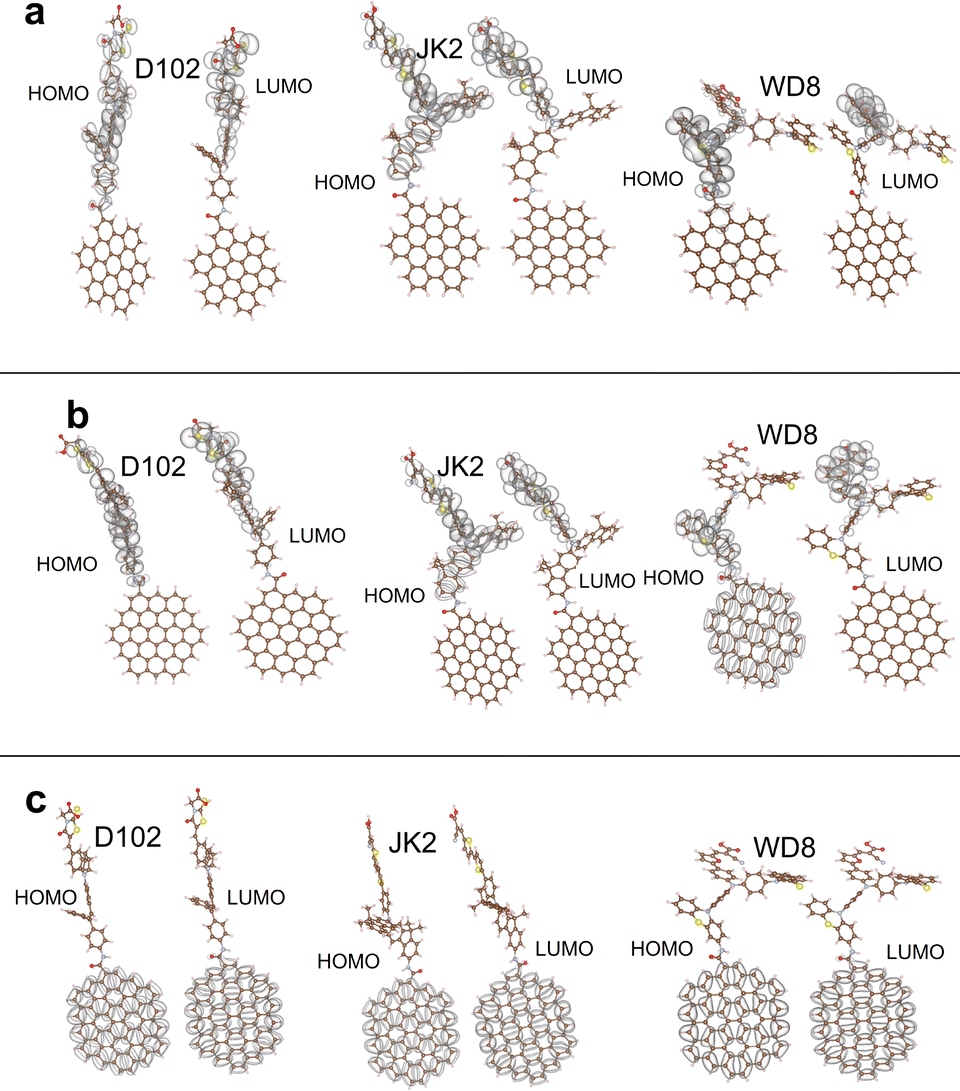Fig. 3 HOMO–LUMO charge distributions for the C42 (a), C54 (b) and C66 (c) nanocomposites. All densities have been obtained with the local hybrid functional Lh12ct-SsifPW92. The isocontour value is chosen as 0.01a₀⁻³.

In summary, we suggest that when matching GQDs and dyes, one needs to carefully study the energy levels in the combined GQD-dye system in order to determine which size of the GQD is suitable for a given dye. While the local hybrid functional used here has been shown to be suitable for dye–TiO₂ interfaces, we recommend testing different functionals for DFT studies of GQD–dye nanocomposites as further validation of density functionals against experimental results or highly accurate theoretical data (e.g. GW or coupled cluster methods) is required. This also means that we cannot reject specific sizes of the GQDs based only on their combination with a few dyes or one density functional approximation.

Fig. 4 shows the Gaussian broadened absorption spectra of the WD8 alone and combined with the different sizes of GQDs. The spectra of the other two dyes (see the ESI†) follow a similar trend and we discuss WD8 explicitly as a representative. First, we note that with the GQDs the overall oscillator strength increases significantly in comparison to the dye alone. The peak corresponding to the absorption maximum of the isolated dye becomes slightly more intense with the B3LYP functional. Also, depending on the functional the maximum oscillator strengths decrease in the following order: CAM-B3LYP > Lh12ct-SsifPW92 > B3LYP. Confirming our observations for the GQD spectra, all three functionals yield comparable spectra that are either entirely shifted towards higher wavelengths (B3LYP) or lower wavelengths (CAM-B3LYP) as compared to Lh12ct-SsifPW92.

Fig. 4 Gaussian broadened absorption spectra of WD8 alone and the WD8-GQD systems obtained with three different exchange correlation functionals.

Table 1 depicts the wavelengths and oscillator strengths of the absorption maxima as well as band-gaps obtained from the difference between the HOMO and LUMO energies. In the last column, light harvesting efficiencies (LHEs) are given for each of the examined systems and different density functional approximation. To calculate the LHEs of the photosensitizers we use Beer's law

LHE = 1 − 10^−f (4)

where f is the oscillator strength linked to the corresponding maximum absorption peak.^56–58 We observe a decrease in band gaps with an increase in the GQD size and compared to the dye alone. The biggest jump is observed switching from C54 to C66. This is in agreement with the orbital pictures showing that the HOMO and LUMO are located on the C66 moiety. The band gap of the C66-dye systems corresponds thus roughly to the one in the isolated C66-GQD (e.g. 2.05 eV vs. 2.06 eV with B3LYP). For the two dyes D102 and JK2, the band gaps of the combined system with the C42-GQD and the C54-GQD are identical and very close to the HOMO–LUMO gap of the isolated dyes. This confirms the observation that both HOMO and LUMO are located on the dyes for these systems. One exception is the C54-D102 system calculated with the CAM-B3LYP functional where the band gap is slightly smaller and the HOMO is located on the graphene sheet. Similar trends have been reported earlier for CAM-B3LYP.⁹

Table 1 Calculated maximum absorption spectra (λ_max), oscillator strengths (f), band-gap (E_g) and light harvesting efficiency (LHE) for each system and functional

Functional	System	λ max [nm]/[eV]	f [vel.]	E g [eV]	LHE
B3LYP	WD8	520/2.38	0.71	2.55	0.8054
	C42-WD8	516.56/2.40	0.80	2.47	0.8402
	C54-WD8	443.62/2.79	1.36	2.45	0.9564
	C66-WD8	487.95/2.54	1.53	2.05	0.9703
CAM-B3LYP	WD8	424/2.92	1.04	4.88	0.9093
	C42-WD8	322.36/3.84	1.68	4.82	0.9791
	C54-WD8	374.77/3.30	2.26	4.50	0.9945
	C66-WD8	403.11/3.07	2.17	3.62	0.9933
Lh12ct-SsifPW92	WD8	474.93/2.61	0.90	3.27	0.8756
	C42-WD8	474.10/2.61	0.98	3.17	0.8968
	C54-WD8	411.68/3.01	1.44	3.13	0.9640
	C66-WD8	450/2.75	1.93	2.48	0.9881
B3LYP	D102	547.71/2.26	1.07	2.49	0.9152
	C42-D102	558.50/2.22	1.25	2.46	0.9443
	C54-D102	444.36/2.79	1.49	2.46	0.9674
	C66-D102	488.67/2.53	1.50	2.05	0.9687
CAM-B3LYP	D102	436.83/2.83	1.60	4.68	0.9751
	C42-D102	439.15/2.82	1.91	4.64	0.9877
	C54-D102	374.67/3.30	2.14	4.53	0.9928
	C66-D102	439.17/2.82	2.39	3.62	0.9959
Lh12ct-SsifPW92	D102	498.84/2.48	1.35	3.09	0.9553
	C42-D102	505.34/2.45	1.60	3.05	0.9751
	C54-D102	504.60/2.45	1.67	3.05	0.9786
	C66-D102	504.66/2.45	1.94	2.48	0.9885
B3LYP	JK2	475/2.61	0.96	2.02	0.8902
	C42-JK2	472.95/2.62	1.00	2.05	0.9008
	C54-JK2	444.60/2.78	1.38	2.05	0.9586
	C66-JK2	486.17/2.55	1.91	1.91	0.9876
CAM-B3LYP	JK2	481.97/2.57	1.72	4.16	0.9811
	C42-JK2	474.47/2.61	1.80	4.19	0.9842
	C54-JK2	374.73/3.30	2.25	4.19	0.9943
	C66-JK2	402.95/3.07	2.28	3.62	0.9948
Lh12ct-SsifPW92	JK2	589.21/2.10	1.09	2.61	0.9189
	C42-JK2	353.95/3.50	1.14	2.63	0.9280
	C54-JK2	413.37/2.99	1.67	2.63	0.9788
	C66-JK2	450/2.75	2.13	2.48	0.9926

---

Next, we compare the wavelengths of the absorption maxima, λ_max, in the UV-Vis spectra of the dyes alone with those of the dye attached to the graphene. In this case, it is more difficult to discern a general trend for shifts. For WD8 and JK2 the absorption maximum is shifted progressively to smaller wavelengths when it is combined with the small GQD and then the medium-sized GQD. Increasing the GQD size from C54 to C66 leads to a notable increase of λ_max for all functionals except Lh12ct-SsifPW92. The latter predicts a smaller λ_max in C42-JK2 as compared to the isolated dye and then a substantial increase of λ_max in the C54-JK2 system. In the case of the D102 dye, all functionals predict a different trend: (i) with the local hybrid (Lh12ct-SsifPW92), the wavelength of the absorption maximum is almost identical (around 505 nm) for all three GQDs. (ii) The range-separated hybrid predicts a similar λ_max value for the isolated dye, C42-D102, and C66-D102 (between 436 and 439 nm) and a considerably smaller wavelength for C54-D102. (iii) With the global hybrid the combination C54-D102 exhibits the smallest λ_max value of 444.36 nm, while the isolated dye and the C42-D102 system feature a larger absorption maximum of 547.71 nm and 558.50 nm, respectively.

Regarding the oscillator strength at the absorption maximum, we observe that it increases consistently upon increasing the size of the graphene sheet. The only exception is found with CAM-B3LYP which yields a higher probability of electronic transition for C54-WD8 than for the C66-WD8 system. Clearly, higher oscillator strengths are leading to greater light harvesting efficiencies [interval 0–1]. Confirming previous findings, CAM-B3LYP predicts the highest efficiencies, followed by the local hybrid functional.

In the next step we anchor different sizes of GQDs to the TiO₂ cluster. Here, the GQD acts as a photosensitizer, which can be confirmed by visualising the spatial HOMO–LUMO charge separation. Indeed, the HOMO is located on the GQD and the LUMO on the TiO₂ in all of the presented cases (Fig. 5).

Fig. 5 HOMO–LUMO charge distributions for the C42, C54 and C66 GQDs together with the TiO₂ cluster with B3LYP. The isocontour value is chosen as 0.01a₀⁻³.

While different sizes of graphene attached to the dyes can significantly influence the electronic structures and thus the mechanism of charge separation, this may change when the nanocomposites are combined with a TiO₂ cluster. In ref. 59 the experimental preparation of DSSCs with a single layer of graphene quantum dots was reported. There the TiO₂ nanoparticles were first coated with GQDs and an organic dye was subsequently added. This suggests that the GQD is bound between the TiO₂ surface and the dye. Following this idea we model the combined system of GQDs and the WD8 dye. First, we investigate the electronic structure through the HOMO and LUMO charge densities for each GQD size system (Fig. 6). We observe different electronic structures depending on the size of the implemented GQD. It is important to note that all of the LUMOs are located on the semiconductor, suggesting a favorable level alignment. The extension of the HOMO densities varies in each case, but they are all located at the dye–GQD system. Appropriate charge separation and a promising feature for their performance in a DSSC are thus indicated. Starting from the first system and the smallest graphene C42, the HOMO is located on the bridge of the WD8 dye with a small fraction on the GQD. Note that this is different from the dye@TiO₂ system, where the HOMO resides on one or both of the donor groups in WD8.²⁷ Moving to the next system with the C54 GQD, the majority of the HOMO density is found on the dye, but it extends significantly to the graphene. In agreement with the visualization of the frontier orbitals of the dye–GQD nanocomposites, the combined system with the largest graphene sheet (C66), exhibits a HOMO completely located on the GQD. As seen from the consistent bandgap in all the dye–GQD, the C66 graphene sheets appears to dominate the charge separation mechanism. In all of these cases, the GQD is serving either as an electron donor or enhancing the dye performance through the transportation of the electrons or light-harvesting ability, reducing the recombination losses in the DSSC system. We show that the role of the graphene can be versatile, depending on the electronic structure of the dye and the interaction with the semiconductor.

Fig. 6 Isocontour of the HOMO and LUMO densities for the WD8@C42@TiO₂, WD8@C54@TiO₂ and WD8@C66@TiO₂ systems with CAM-B3LYP. The isocontour value is chosen as 0.01a₀⁻³.

For an efficient DSSC, a strong light absorption in the visible spectra is required before the electron can be injected into the conduction band of the semiconductor. We have thus computed the UV-Vis spectra of the WD6@GQD@TiO₂ systems as well. Considering the computational costs, we only allow excitations from the HOMO, while lower occupied orbitals are kept frozen (except WD8@TiO₂, where excitations from all occupied orbitals are allowed). Fig. 7 shows the absorption spectra of the WD8@TiO₂, WD8@C42@TiO₂, WD8@C54@TiO₂ and WD8@C66@TiO₂ systems with the B3LYP, CAM-B3LYP and Lh12ct-SsifPW92 functionals. First, we notice that the spectra of the WD8@TiO₂ system without GQD is barely visible due to the lower oscillator strength in comparison to the systems with graphene. With the global hybrid B3LYP and the local hybrid (Lh12ct-SsifPW92) all absorption maxima are predicted to lie in the in visible range of light while the total absorption range is significantly narrower and overall blue-shifted with CAM-B3LYP. The same behaviour was seen for the dye–GQD systems (cf.Fig. 4). Also in agreement with our previous observation for the dye@GQD systems, the spectra of the composite with the largest GQD (C66) are red-shifted with all functionals.

Fig. 7 Absorption spectra of the WD8 dye together with the TiO₂ semiconductor and different sizes of GQDs, calculated with B3LYP, CAM-B3LYP and Lh12ct-SsifPW92 functionals. Spectra are obtained by allowing only excitations from the HOMO, while lower orbitals are kept frozen.

Depending on the functional, we find that different GQDs lead to higher intensities: with B3LYP the WD8@C54@TiO₂ system features the most intense absorption followed by the WD8@C42@TiO₂ model, with CAM-B3LYP this system is almost on par with the C66-containing DSSC model, and the local hybrid (Lh12ct-SsifPW92) clearly predicts the WD8@C66@TiO₂ system to exhibit the largest oscillator strengths. The light absorption of the latter is more than 10 times more efficient than that of the C54@GQD based model, and the spectra of the WD8@C42@TiO₂ system shows vanishingly small intensities in comparison.

Compared to ref. 16 where the authors observed a significant reduction in the oscillator strengths of the combined dye@GQD@TiO₂ systems, our study is offering a different perspective, one possible reason for this behaviour can be stronger hybridization between the dye and the semiconductor states with the smaller (TiO₂)₁₅ cluster used in ref. 16 or the influence of the functional on the absorption intensity. In our previous studies, we already mentioned the importance of the optimal size of the TiO₂ cluster and its influence on the charge transfer dynamics.^25,27

In the following, we will focus on the WD8@C66@TiO₂ system, as it is according to the calculations with CAM-B3LYP and Lh12ct-SsifPW92 the best candidate for DSSCs. Fig. 8 shows the comparison between the two absorption spectra calculated with CAM-B3LYP and Lh12ct-SsifPW92 functionals. Despite a general red-shift and slightly higher oscillator strengths with the local hybrid, both functionals predict the same maximum absorption peak at 458 nm.

Fig. 8 Absorption spectra of the WD8@C66@TiO₂ system with the CAM-B3LYP and Lh12ct-SsifPW92 functionals.

We have seen that for C66 GQD in combination with the WD8 dye and the TiO₂ cluster, the HOMO density resides always on the graphene sheet (cf.Fig. 5 and 6). Although the dye may not contribute directly to charge separation, it can still enhance the spectral properties. We therefore inspect the role of the dye in the bigger system by comparing the UV-Vis spectra of the WD8-C66-TiO₂ and the C66-TiO₂ system in Fig. 9. Most importantly, the spectra of the bigger system are favorably red-shifted but also narrower. For example, an intense peak at about 560 nm, in the spectra of the C66-TiO₂ system vanishes upon the addition of the dye. We conclude that the addition of the dye introduces stronger electronic coupling between C66 and WD8, resulting in fewer, more intense peaks (Fig. 9).

Fig. 9 Absorption spectra of the C66@TiO₂ and WD8@C66@TiO₂ system with the CAM-B3LYP functional.

In addition to spectroscopic properties, and to better understand the role of WD8 and its interaction with C66 in the whole system, we calculated the binding energy of WD8 on C66@TiO₂, using the expression

E_b = E_WD8@C66@TiO2 − (E_C66@TiO2 + E_WD8) (5)

The calculated binding energy between WD8 and C66 is −15.33 eV, corresponding to a strong chemical interaction (chemisorption).

Additionally, we analyzed the driving force of electron injection, ΔG^inject, for our WD8@C66@TiO₂ system to quantify the thermodynamic feasibility and efficiency of electron injection, which is −4.37 eV.^60–63

ΔG^inject = (−E^WD8@C66_HOMO − λ_max) − E_CB (6)

Here, E^WD8@C66_HOMO equals the HOMO energy of the separate WD8@C66 nanocomposite, λ_max is the absorption maximum of the combined WD8@C66@TiO₂ system and E_CB is taken as −4.2 eV, i.e. the experimental energy of the conduction band in TiO₂. This negative value suggests a thermodynamically favorable driving force for effective electron injection. To estimate the speed of the injection, explicit electron dynamics calculations will be carried out in future work.

As a pioneering investigation into complex systems incorporating GQDs within DSSCs, we also analyzed the energy level alignments using three different functionals (Fig. 10). In contrast to our previously calculated level alignments for WD8@TiO₂, an intermediate energy level, the C66-LUMO emerges. It changes the possible electron transfer pathways. Since graphene has a versatile function, possible injection paths are from the WD8-LUMO to the C66-LUMO, if graphene acts as a mediator or directly from the C66-LUMO into the semiconductor, if the exciton is generated solely on the graphene moiety. Given the energy of the excitation maxima in the UV-Vis spectra, excitation into the dye LUMO appears to be more likely. Interestingly, all three functionals provide qualitatively the same level alignments and would allow for either mechanism. As mentioned before, a more detailed picture of the charge injection upon excitation of the system can also be obtained through electron dynamics calculations.

Fig. 10 Alignment of the energy levels in the WD8@C66@TiO₂ system from LR-TDDFT calculations with three different functionals labeled in the figure: B3LYP, CAM-B3LYP and Lh12ct-SsifPW92.

5. Conclusion and outlook

In this work we systematically approach the idea of implementing graphene in the form of GQDs inside DSSCs to enhance the photovoltaic efficiency of the system. Thus, we considered three different sizes of GQDs, C42, C54 and C66, and studied their electronic structure and UV-Vis spectra also in combination with three different dyes and a large TiO₂ cluster.

With the standard exchange–correlation functional, the calculated absorption maxima of the smallest GQD closely matched the experimental value. Increasing the size of the sheet, a red-shift of the absorption maximum can be seen and for the largest, C66, additional peaks at higher wavelengths appear in the UV-Vis spectra hinting at more complex quantum confinement effects. Attaching three different types of dyes (D102, JK2 and WD8) to the GQDs, and inspecting the respective HOMO and LUMO densities confirms that no general recommendation about the desirable size of a GQD can be made. Instead, the spatial extension of the frontier orbitals depends on the dye and also the underlying density functional approximation. For the largest GQD, all functionals predict the localization of the HOMO and LUMO on the graphene part, while the picture is mixed for the medium-sized GQD, and for the smallest the HOMO and LUMO reside consistently on the dyes. Our TDDFT calculation revealed a significant increase in the oscillator strengths for the dye@GQD system in comparison to the dye alone and the probability of excitation becomes stronger when the sheet is larger.

For the combined dye@GQDs@TiO₂ systems we focused on the dye WD8. Here, an interesting behaviour with an increase in the GQD size was observed: the HOMO density is slowly shifted from the WD8 dye (WD8@C42@TiO₂) to the graphene (WD8@C54@TiO₂) and then located at the graphene exclusively (WD8@C66@TiO₂). The LUMO is always located on the semiconductor indicating good charge separation and favorable level alignment which are both needed for the DSSC functionality. To gain a better understanding of the role of GQDs in combination with an organic dye in a DSSC, we have also studied the three WD8@GQD@TiO₂ systems. The most notable effect of the GQD is a considerable increase in oscillator strength, where different density functionals predict different GQDs to be most promising, i.e. showing the highest absorption intensities. The level alignment of the WD8@C66@TiO₂ system shows that a possible charge injection involves exciting an electron from the HOMO that is located on the GQD to either the LUMO of the GQD or the dye followed by injection into the lower lying LUMO of the TiO₂ cluster. Further studies are required to understand the role of the dye in this system. Even if it is not contributing directly to the exciton generation, the dye might still improve spectral properties through the light harvesting ability, overall transition dipole moment, reduce recombination losses, etc. In particular to analyze the latter, electron dynamics calculations are envisioned. Also extending our studies to differently structured dyes and larger graphene sheets is subject to future work.

Author contributions

D. Gemeri: writing – original draft, conceptualization, visualization, data curation, and investigation; Ž. S. Maršić: writing – review & editing; H. Bahmann: writing – review & editing, conceptualization, and funding acquisition.

Data availability

The data supporting this article have been included as part of the ESI.†

Conflicts of interest

There are no conflicts to declare.

Acknowledgements

H. B. acknowledges funding by Deutsche Forschungsgemeinschaft (DFG, the German Research Foundation) – project no. 418140043. This research was partially supported under the project STIM – REI, Contract Number: KK.01.1.1.01.0003, a project funded by the European Union through the European Regional Development Fund – the Operational Programme Competitiveness and Cohesion 2014-2020 (KK.01.1.1.01).

References

1. K. S. Novoselov, A. K. Geim, S. V. Morozov, D. Jiang, Y. Zhang, S. V. Dubonos, I. V. Grigorieva and A. A. Firsov, Science, 2004, 306, 666–669.
2. L. A. Ponomarenko, F. Schedin, M. I. Katsnelson, R. Yang, E. W. Hill, K. S. Novoselov and A. K. Geim, Science, 2008, 320, 356–358.
3. X. Xu, R. Ray, Y. Gu, H. J. Ploehn, L. Gearheart, K. Raker and W. A. Scrivens, J. Am. Chem. Soc., 2004, 126, 12736–12737.
4. D. Wang, J.-F. Chen and L. Dai, Part. Part. Syst. Charact., 2015, 32, 515–523.
5. X. Yan, X. Cui, B. Li and L.-S. Li, Nano Lett., 2010, 10, 1869–1873.
6. L.-S. Li and X. Yan, J. Phys. Chem. Lett., 2010, 1, 2572–2576.
7. M. Li, W. Wu, W. Ren, H.-M. Cheng, N. Tang, W. Zhong and Y. Du, Appl. Phys. Lett., 2012, 101, 103107.
8. S. Kim, S. W. Hwang, M.-K. Kim, D. Y. Shin, D. H. Shin, C. O. Kim, S. B. Yang, J. H. Park, E. Hwang, S.-H. Choi, G. Ko, S. Sim, C. Sone, H. J. Choi, S. Bae and B. H. Hong, ACS Nano, 2012, 6, 8203–8208.
9. F. Gao, C.-L. Yang, M.-S. Wang, X.-G. Ma and W.-W. Liu, Spectrochim. Acta, Part A, 2019, 206, 216–223.
10. F. Gao, C.-L. Yang, M.-S. Wang, X.-G. Ma and W.-W. Liu, Spectrochim. Acta, Part A, 2019, 216, 69–75.
11. Y. Zhang, H. Li, L. Kuo, P. Dong and F. Yan, Curr. Opin. Colloid Interface Sci., 2015, 20, 406–415.
12. E. Singh and H. S. Nalwa, Sci. Adv. Mater., 2015, 7, 1863–1912.
13. R. Ghayoor, A. Keshavarz, M. N. S. Rad and A. Mashreghi, Mater. Res. Exp., 2018, 6, 025505.
14. A. J. Nozik, Chem. Phys. Lett., 2008, 457, 3–11.
15. N. Sohal, B. Maity and S. Basu, RSC Adv., 2021, 11, 25586–25615.
16. F. Gao, C.-L. Yang and G. Jiang, J. Photochem. Photobiol., A, 2020, 407, 113080.
17. M. Yang, Z. Lian, C. Si and B. Li, Phys. Chem. Chem. Phys., 2020, 22, 28230–28237.
18. B. Li, Y. Wang, L. Huang, H. Qu, Z. Han, Y. Wang, M. J. Kipper, L. A. Belfiore and J. Tang, Synth. Met., 2021, 276, 116758.
19. F. Gao, C.-L. Yang, M.-S. Wang, X.-G. Ma and W.-W. Liu, Spectrochim. Acta, Part A, 2019, 206, 216–223.
20. G. Williams, B. Seger and P. V. Kamat, ACS Nano, 2008, 2, 1487–1491.
21. K.-W. Min, M.-T. Yu, C.-T. Ho, P.-R. Chen, J.-K. Tsai, T.-C. Wu and T.-L. Wu, Mod. Phys. Lett. B, 2022, 36, 2141017.
22. S. Mahalingam, A. Manap, K. Lau, A. Omar, P. Chelvanathan, C. Chia, N. Amin, I. Mathews, N. Afandi and N. Rahim, Electrochim. Acta, 2022, 404, 139732.
23. S. Mahalingam, A. Manap, R. Rabeya, K. S. Lau, C. H. Chia, H. Abdullah, N. Amin and P. Chelvanathan, Electrochim. Acta, 2023, 439, 141667.
24. M. Pastore and F. De Angelis, Phys. Chem. Chem. Phys., 2012, 14, 920–928.
25. D. Gemeri, J. C. Tremblay, M. Pastore and H. Bahmann, Chem. Phys., 2022, 559, 111521.
26. D. Sun, C. Yang, T. Liu and Y. Li, Adv. Theory Simul., 2023, 6, 2200940.
27. D. Gemeri, J. C. Tremblay and H. Bahmann, Adv. Quantum Chem., 2023, 88, 329–350.
28. A. D. Becke, J. Chem. Phys., 1993, 98, 1372–1377.
29. T. Yanai, D. P. Tew and N. C. Handy, Chem. Phys. Lett., 2004, 393, 51–57.
30. T. M. Maier, A. V. Arbuznikov and M. Kaupp, Wiley Interdiscip. Rev.: Comput. Mol. Sci., 2019, 9, e1378.
31. S. G. Balasubramani, G. P. Chen, S. Coriani, M. Diedenhofen, M. S. Frank, Y. J. Franzke, F. Furche, R. Grotjahn, M. E. Harding, C. Hättig, A. Hellweg, B. Helmich-Paris, C. Holzer, U. Huniar, M. Kaupp, A. Marefat Khah, S. Karbalaei Khani, T. Müller, F. Mack, B. D. Nguyen, S. M. Parker, E. Perlt, D. Rappoport, K. Reiter, S. Roy, M. Rückert, G. Schmitz, M. Sierka, E. Tapavicza, D. P. Tew, C. van Wüllen, V. K. Voora, F. Weigend, A. Wodyński and J. M. Yu, J. Chem. Phys., 2020, 152, 184107.
32. M. D. Hanwell, D. E. Curtis, D. C. Lonie, T. Vandermeersch, E. Zurek and G. R. Hutchison, J. Cheminf., 2012, 4, 17.
33. K. Momma and F. Izumi, J. Appl. Crystallogr., 2008, 41, 653–658.
34. V. A. Rassolov, M. A. Ratner, J. A. Pople, P. C. Redfern and L. A. Curtiss, J. Comput. Chem., 2001, 22, 976–984.
35. C. Lee, W. Yang and R. G. Parr, Phys. Rev. B: Condens. Matter Mater. Phys., 1988, 37, 785–789.
36. A. Schäfer, A. Klamt, D. Sattel, J. C. W. Lohrenz and F. Eckert, Phys. Chem. Chem. Phys., 2000, 2, 2187–2193.
37. E. Ronca, M. Pastore, L. Belpassi, F. Tarantelli and F. De Angelis, Energy Environ. Sci., 2013, 6, 183–193.
38. N. Martsinovich, D. R. Jones and A. Troisi, J. Phys. Chem. C, 2010, 114, 22659–22670.
39. A. V. Arbuznikov and M. Kaupp, J. Phys. Chem. C, 2012, 136, 014111.
40. H. Bahmann and M. Kaupp, J. Chem. Theory Comput., 2015, 11, 1540–1548.
41. T. M. Maier, H. Bahmann and M. Kaupp, J. Chem. Theory Comput., 2015, 11, 4226–4237.
42. J. L. Bao, L. Gagliardi and D. G. Truhlar, J. Phys. Chem. Lett., 2018, 9, 2353–2358.
43. H. Bahmann, Chall. Det. Appr. Foren. Sci., 2021, 20, 165.
44. A. Dreuw and M. Head-Gordon, J. Am. Chem. Soc., 2004, 126, 4007–4016.
45. A. Dreuw, J. L. Weisman and M. Head-Gordon, J. Chem. Phys., 2003, 119, 2943–2946.
46. M. J. G. Peach, P. Benfield, T. Helgaker and D. J. Tozer, J. Chem. Phys., 2008, 128, 044118.
47. A. Karolewski, T. Stein, R. Baer and S. Kümmel, J. Chem. Phys., 2011, 134, 151101.
48. J. Jaramillo, G. E. Scuseria and M. Ernzerhof, J. Chem. Phys., 2003, 118, 1068–1073.
49. E. Clar and W. Schmidt, Tetrahedron, 1977, 33, 2093–2097.
50. X. Yan, X. Cui and L.-S. Li, J. Am. Chem. Soc., 2010, 132, 5944–5945.
51. J. W. Patterson, J. Am. Chem. Soc., 1942, 64, 1485–1486.
52. D. Medina-Lopez, T. Liu and S. Osella, et al. , Nat. Commun., 2023, 14, 4728.
53. T. Fan, L. Jian, X. Huang, S. Zhang, I. Murtaza, R. Abid, Y. Liu and Y. Min, J. Mater. Sci.: Mater. Electron., 2022, 33, 1–11.
54. C. Yu, H. Fang, Z. Liu, H. Hu, X. Meng and J. Qiu, Nano Energy, 2016, 25, 184–192.
55. B. Wang, A. Song, L. Feng, H. Ruan, H. Li, S. Dong and J. Hao, ACS Appl. Mater. Interfaces, 2015, 7, 6919–6925.
56. W. Fan, D. Tan and W.-Q. Deng, Chem. Phys. Chem., 2012, 13, 2051–2060.
57. R. Katoh, A. Furube, T. Yoshihara, K. Hara, G. Fujihashi, S. Takano, S. Murata, H. Arakawa and M. Tachiya, J. Phys. Chem. B, 2004, 108, 4818–4822.
58. D. F. Swinehart, J. Chem. Educ., 1962, 39, 333.
59. F. Jahantigh, S. B. Ghorashi and A. Bayat, Dyes Pigm., 2020, 175, 108118.
60. H. Gerischer, M. Michel-Beyerle, F. Rebentrost and H. Tributsch, Electrochim. Acta, 1968, 13, 1509–1515.
61. H. Tributsch and M. Calvin, Photochem. Photobiol., 1971, 14, 95–112.
62. J. Conradie, Energy Nexus, 2024, 13, 100282.
63. Y. Li, L. Mi, H. Wang, Y. Li and J. Liang, Materials, 2019, 12, 193.

---

Footnote

† Electronic supplementary information (ESI) available. See DOI: https://doi.org/10.1039/d5ma00246j

---