Machine learning prediction of self-assembly and analysis of molecular structure dependence on the critical packing parameter

Abstract

Amphiphilic molecules spontaneously form self-assembly structures depending on physical conditions such as the molecular structure, concentration, and temperature. These structures exhibit various functionalities according to their morphology. The critical packing parameter (CPP) is used to correlate self-organized structures with the chemical composition. However, accurately calculating it requires information about both the molecular shape and molecular aggregates, making it challenging to apply directly in molecular design. We aimed to predict the self-assembled structure of a molecule directly from its chemical structure and to analyze the factors influencing it using machine learning. Dissipative particle dynamics simulations were used to reproduce many self-assembly structures comprising various chemical structures, and their CPPs were calculated. Machine learning models were built using the chemical structures as input data and the CPPs as output data. As a result, both random forest and the gated recurrent unit showed high prediction accuracy. Feature importance analysis and sample size dependence revealed that the amphiphilic nature of molecules significantly influences the self-assembly structures. Additionally, selecting an appropriate molecular structure representation for each algorithm is crucial. The study results should contribute to product development in the fields of materials science, materials chemistry, and medical materials.

---

Design, System, Application

Functional materials utilizing amphiphilic molecules are widely applied in various fields. The functionalities of amphiphilic molecules are achieved through their spontaneous self-assembly, resulting in different functions depending on the structures formed. Self-assembly structures depend not only on the molecular structure but also on experimental conditions such as temperature and concentration. Predicting self-assembly structures tailored to specific functions from molecular chemical structures is challenging, and trial-and-error molecular design remains the mainstream approach in product development. In this study, we combined molecular simulations with machine learning to directly predict self-assembly structures from molecular structures. Furthermore, by analyzing the input data for machine learning, we revealed the essential factors influencing self-assembly structures. This enables the prediction of self-assembly structures at the molecular design stage, which indicates the potential to predict the functions that arise from these structures at the molecular design stage. This advancement has the potential to significantly reduce the cost of product development. Additionally, the results of this machine learning research are expected to provide valuable insights not only in the field of materials science but also in the field of materials informatics.

1 Introduction

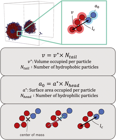
Amphiphilic molecules have attracted significant attention as functional materials¹ and have been applied in various fields such as materials chemistry^2–4 and medical materials science.^5–7 For example, their functional properties have been exploited for applications such as detergents and liposomes used as drug delivery carriers.⁸ The functionalities of amphiphilic molecules are achieved through the self-assembly structures formed by their spontaneous aggregation. For example, in detergent micelles, the hydrophobic tails adsorb oils and the hydrophobic cores trap oil stains. Liposomes used as drug carriers can encapsulate water-soluble substances and release them under specific conditions. Other self-assembled structures, such as threadlike micelles^9,10 and bilayer membranes,^11,12 exhibit distinctive intrinsic properties that are being actively investigated for various applications. However, designing such self-assembled structures for achieving desired functions remains challenging as they depend not only on the chemical structure of the molecules but also on physical parameters such as concentration and temperature. As a result, a definitive method has not yet been established for achieving desired functionalities; consequently, time-consuming and costly trial-and-error experiments are still required. Predicting and controlling the self-assembly of amphiphilic molecules is therefore a critical engineering task.

The critical packing parameter (CPP) links the chemical structure of molecules to self-assembled structures.¹³ The CPP is a dimensionless quantity that represents the geometric balance of hydrophilic and hydrophobic moieties at the interface of self-assembled structures. It is defined in terms of the surface area of the hydrophilic part (a₀), the volume of the hydrophobic part (v), and the critical chain length (l_c) as CPP = v/a₀l_c. The CPP plays a crucial role in determining the type of self-assembled structure formed. For example, when 0 < CPP < 1/3, micelles form; 1/3 < CPP < 1/2 results in thread-like micelles; 1/2 < CPP < 1 results in vesicles or flexible bilayer membranes; and CPP ∼ 1 results in planar bilayer membranes. However, accurately calculating the CPP from only the molecular structure is challenging owing to the influence of other thermodynamic conditions on self-assembled structures. Experimental estimates of the CPP often deviate from estimated values, thus necessitating a reliance on experimental observations to infer the structure. Therefore, accurate calculation of the CPP requires the consideration of both the molecular shape and the self-assembly information, making direct application to molecular design difficult. Consequently, to the best of our knowledge, self-assembled structures have not yet been accurately predicted using CPPs estimated solely from molecular structure information.

Machine learning technology enables computers to iteratively learn from given data and to uncover patterns within them, thus allowing predictions of unknown data. In recent years, artificial intelligence technology has found widespread applications in various fields, including for soft matter and molecular simulations in materials informatics.^14–19 Inokuchi et al.²⁰ successfully predicted the properties of surfactants by using a combination of molecular simulations and machine learning. This demonstrates the applicability of machine learning even to complex systems containing self-assembled structures of amphiphilic molecules. Bhattacharya et al.²¹ identified monomer sequences for self-assembling copolymers that form specific morphologies. However, these studies were limited to linear molecular models or only with a small amount of branches,²² and the feasibility of applying machine learning to molecular models of amphiphilic molecules with complex structures such as branching or cyclic structures remained unclear.

The present study focuses on the CPP and aims to combine machine learning and molecular simulation for predicting self-assembled structures formed in water. The CPP has not yet been used to accurately predict the self-assembly structure of amphiphilic molecules. Our target is molecular models of amphiphilic molecules with complex structures, including branching and cyclic structures, in addition to linear structures. We aim to demonstrate the feasibility of applying machine learning to these complex molecular structures. We examined the input data for machine learning to identify the main factors affecting self-assembly. This enabled us to predict the resultant self-assembled structures without requiring trial-and-error experiments. The results should contribute to the molecular design of functional materials and the advancement of materials science.

2 Methods

2.1 Molecular simulation

We used the dissipative particle dynamics (DPD) simulation technique^23–26 to study the self-assembly behavior of amphiphilic molecules. DPD was specifically developed to simulate the fluidic and thermodynamic behaviors of various aqueous solutions. DPD is a particle-based method that uses coarse-grained models in which atoms and molecules are lumped together as DPD beads for efficiency, thus offering a computational advantage over classical molecular dynamics. In particular, DPD has produced various successful results regarding the self-assembly of amphiphilic molecules.^27–29

The DPD method uses Newton's equation of motion with conservative, dissipative, and random forces applied to all DPD beads. Newton's equation of motion for particle i is

where m is the particle mass, v is the particle velocity, F^C is the conservative force, F^R is the pairwise random force, and F^D is the dissipative force. The conservative force F^C is given by the following equation.where r_ij = r_j − r_i and n_ij = r_ij/∣r_ij∣. a_ij is the parameter that determines the magnitude of the repulsive force between particles i and j, and r_c is the cutoff distance to determine the effective range of force. The random force (F^R_ij) and dissipative force (F^D_ij) are respectively given bywhere v_ij = v_j − v_i, σ is the noise parameter, γ is the friction parameter, and ζ_ij is a random number based on a Gaussian distribution. Here, ω^R and ω^D are r-dependent weight functions given as follows.

The temperature is controlled by a couple of dissipative and random forces. σ and γ are related by the fluctuation–dissipation theorem as

σ² = 2γk_BT, (6)

where k_B is Boltzmann's constant and T is the temperature. In DPD simulations, reduced units are generally used.

In this study, we adopted the spring force F^S_ij defined as

where r_s is the equilibrium bond distance representing the bond between linked DPD beads in the modeled molecules and k_s is the spring constant.

In DPD simulations, a reduced unit system is typically employed. In this context, the length is given in terms of the cutoff distance r_c, the mass is given in terms of the bead mass m, and energy is represented in units of k_BT. The DPD time scale is defined as τ = r_c(m/k_BT)^1/2. To correlate the simulation results with real-world systems, a scaling procedure for length and time units is applied.³⁰ In this simulation, the coarse-graining of three water molecules into a single DPD particle results in a mass unit equivalent to 54 atomic mass units. The particle density in the simulation is set as ρr³_c = 3. This implies the inclusion of three DPD particles within the cube of r³_c, corresponding to a volume of 0.27 nm³, since the volume of a water molecule is 0.03 nm³. Consequently, the length unit r_c is 0.27^1/3 nm = 0.6463 nm, and an approximate DPD time scale τ ≈ 88 ps can be assumed.

2.2 Simulation models and conditions

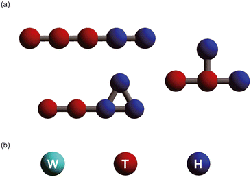
A wide variety of amphiphilic molecule models were created by changing the number of coarse-grained particles and the arrangement of hydrophilic and hydrophobic groups. Fig. 1 shows the simulation models used in this study. Typical amphiphilic molecular models are shown in Fig. 1[a]. These models include linear, cyclic, and branching structures. In total, 305 amphiphilic molecular models were used in the simulations. A water molecule (W) is represented as a single coarse-grained particle, as shown in Fig. 1[b]. The red and blue particles in the amphiphilic molecular models respectively represent hydrophobic tail groups (T) and hydrophilic head groups (H). The interaction parameters (a_ij) between each pair of particles are shown in Table 1.

Fig. 1 Particle models used for calculations. (a) Representative modeled amphiphilic molecules composed of two types of DPD beads: hydrophobic tail (red) and hydrophilic head (blue). (b) Coarse-grained DPD beads used in this study. The water bead as solvent (cyan), hydrophobic tail bead (red), and hydrophilic head bead (blue) are labeled W, T, and H, respectively.

Table 1 Interaction parameters a_ij (in k_BT/r_c units) in DPD calculations

	W	T	H
W	25.0	75.0	25.0
T		25.0	75.0
H			25.0

---

The nearest neighboring particles within the modeled amphiphilic molecules are connected by harmonic springs with a spring constant of 100k_BT/r²_c and an equilibrium length of 0.86r_c. The concentration of the aqueous solution is set at 5%. The number of coarse-grained DPD beads in the modeled amphiphilic molecules and water molecules is 4050 and 76 950, respectively. In this system, a random initial configuration was employed. The simulation box has a volume of 30 × 30 × 30r³_c, with periodic boundary conditions applied in all three dimensions. All simulations were conducted in a constant-volume and constant-temperature ensemble until the equilibrium state was reached in 16 000τ.

2.3 Machine learning

In this study, we have used regression analysis as a form of supervised learning to predict self-assembled structures derived from a coarse-grained molecular model. Specifically, we evaluated well-established regression models including Lasso and Ridge, both of which are variants of linear regression with regularization techniques: support vector regression (SVR), which is based on a support vector machine (SVM) framework, kernel-based methodologies such as the k-nearest neighbor (k-NN) approach, ensemble techniques such as the random forest algorithm, and broader regression frameworks including neural networks (NNs) and the subclass of recurrent neural networks (RNNs). All except NNs and RNNs are implemented using the scikit-learn package,³¹ while NNs and RNNs are implemented using pytorch.³²

In all instances, an ensemble of models was trained via cross-validation on a dataset consisting of 305 samples. Structural data originating from coarse-grained molecular models were used as input datasets, and the CPPs were the outputs. For coarse-grained molecular model structures to be used as inputs, they must first be transformed into a machine-readable format. We used the simplified molecular input line entry system (SMILES), a methodology for linearly encoding chemical structures, to facilitate the conversion of the structural data of the coarse-grained molecular models into a suitable form for our analyses.

Next, the hyper-parameters for each model need to be optimized. Considering the limited extent of the dataset, we used the exhaustive grid search technique. The resulting parameter permutations include those hyper-parameters that yield the highest coefficient of determination (R²).

2.4 Encoding for machine learning

Chemical structures must be encoded into a readable format for machine learning. We encoded the amphiphilic molecule models based on the SMILES notation. The SMILES^33–35 is widely used for converting chemical structures into linear notations, especially when entering chemical information into databases. It represents molecular information as a single string that is easily understandable for both humans and computers. The structures are transformed into strings according to specific rules, including the following key ones:

1. Atoms are denoted by their elemental symbols. Hydrogen atoms are usually omitted but can be explicitly indicated if necessary.

2. Single bonds are implicit, and two adjacent atoms are automatically considered singly bonded. Double and triple bonds are respectively represented by “=” and “#”.

3. Branching structures are typically indicated using parentheses. For instance, acetic acid is represented as CC(=O)O.

4. Absolute configurations are denoted by “@” or “@@”, and geometric isomerism is indicated using “/” or “\”.

5. Ring structures are represented as broken chains, with break points indicated by numbers. For example, cyclohexane is written as C1CCCCC1.

6. In aromatic rings, constituent elements are represented by lowercase letters. For example, benzene is written as c1ccccc1.

Further rules have been defined for the conversion of various structures. We adopted the following modified method called the “modified-SMILES” that used simpler rules than those of the conventional SMILES for converting coarse-grained molecular models into a linear notation while still capturing necessary information adequately.

1. Hydrophobic and hydrophilic bead particles are respectively represented by 1 and 2.

2. All connections between particles have the same spring constant and are therefore represented by adjacent particle symbols.

3. Branching structures are represented using 0 instead of parentheses.

4. Similar to the SMILES, ring structures are represented as broken chains with break points indicated by numbers, except that the break points are set to 9.

By following these rules, we can represent the straight chains, branching, and ring structures in the coarse-grained molecular model in a linear notation. Specific examples are shown in Fig. 2.

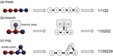Fig. 2 Modified-SMILES for the linear transformation of coarse-grained molecular models; linear transformation methods for (a) linear, (b) branched, and (c) ring structures.

3 Results and discussion

3.1 Analysis of self-assembly structures and the CPP

The simulations revealed a variety of self-assembled structures, including micelles and vesicles, depending on the molecular structure. To determine the CPP, as defined below, we obtained the surface area of the hydrophilic portion (a₀), the volume of the hydrophobic portion (v), and the critical chain length (l_c) from the self-assembled structures generated during the simulations.Among the multiple clusters present within the system, we selected the self-assembled structure with the highest aggregation number. Fig. 3 shows the method for calculating the three values required to determine the CPP from the simulation results. The volume (v) was computed by multiplying the volume occupied by a single hydrophobic particle by the number of hydrophobic particles within a single molecule. To obtain the volume per particle, we assumed a uniform particle distribution with a density of ρ = 3 and a constant number of particles within the system. For calculating the surface area (a₀), we multiplied the number of hydrophilic particles in contact with water by the surface area per particle. The surface area per particle was derived by taking the two-thirds power of the volume per particle to perform a dimensional conversion. The critical chain length (l_c) was defined as the distance between the center of mass of the molecule and the farthest hydrophobic particle as well as the closest hydrophilic particle. We used these calculated values to obtain the CPPs for all amphiphilic molecular models and verified the corresponding values for each self-assembled structure (Fig. 4).

Fig. 3 Calculation method for obtaining the three values needed to calculate the CPP.

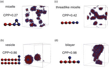Fig. 4 Representative snapshots of equilibrium morphologies of amphiphilic molecules and CPPs of their models: (a) micelle, (b) vesicle, (c) threadlike micelle, and (d) bilayer.

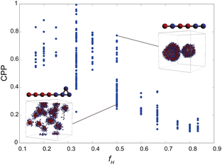
As the CPP of an aggregate is derived from parameters such as the surface area occupied by hydrophilic groups and the volume encapsulated by hydrophobic moieties, the relative abundance of hydrophilic and hydrophobic components within the molecule is expected to strongly influence the resultant self-assembled configuration. In fact, the proportion of hydrophilic or hydrophobic groups in a diblock copolymer greatly affects their self-assembly.^36,37 Accordingly, we focused on a fraction of the hydrophilic portion and plotted a scatter diagram of the CPP obtained from simulations against the ratios of hydrophilic head particles within each molecule (f_H) in Fig. 5. This figure reveals a notable negative correlation with a coefficient of −0.826 between the CPP and the fraction of hydrophilic groups (f_H). This correlation can be attributed to the increased surface area (a₀) occupied by hydrophilic particles as their fraction increases. However, even when the fraction of hydrophilic groups is kept constant, significant variations occur in self-assembled structures owing to differences in factors such as the arrangement of particles, the number of constituent particles, branching structures, and the presence of ring structures. This suggests that factors other than the fraction of hydrophilic groups also play a crucial role in determining the self-assembled structures. In fact, for the same fraction of hydrophilic groups (f_H = 0.5), differences in the locations of ring or branching structures have been found to influence the CPP. For example, if a molecule has a ring structure consisting of hydrophobic tail beads, its critical chain length l_c should be shorter than that of a molecule without a cyclic structure, resulting in a larger CPP. If a molecule has branches with hydrophilic head beads, the surface area of the hydrophilic portion a₀ will be larger, making the CPP smaller. As such, various interrelated parameters must be considered in determining the self-assembled structure, making it difficult to predict the self-assembled behavior from the molecular structure. Thus, we used machine learning methods to analyze and discover key factors to clarify the relationship between the molecular structure and its self-assembly in terms of the CPP. This approach will enable us to not only predict the self-assembly but also manipulate the self-assembly of amphiphiles through molecular design.

Fig. 5 Scatter diagrams of correlation between the CPP and the fraction of hydrophilic head groups.

3.2 Machine learning prediction

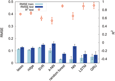
We evaluated the performance of the following machine learning algorithms, including deep learning methods: Lasso,³⁸ Ridge,^39,40k-NN,⁴¹ SVR,⁴² random forest,⁴³ fully connected NNs,⁴⁴ long short-term memory (LSTM),⁴⁵ and gated recurrent unit (GRU).⁴⁶ Lasso and Ridge are regression techniques that add regularization to linear models to prevent overfitting and handle multicollinearity. They mainly differ in terms of the use of distinct regularization methods. Lasso regression shows good performance for feature selection by effectively eliminating redundant attributes. By contrast, Ridge regression mitigates overfitting, thereby improving the overall stability of the model. In this study, considering the limited dataset size of 305, linear regression models were also included for comparison. The other models are all nonlinear. k-NN is a regression algorithm that predicts the value of a new data point by considering the average (or weighted average) of the target variable of k nearest-neighbor data points. SVR is an SVM-based regression model that finds a hyperplane to predict the target variable while maximizing the margin with data points. SVR handles linear and nonlinear relationships using kernel functions, making it suitable for high-dimensional data and complex regression tasks. Random forest is an ensemble learning method that introduces randomness to data and feature selection to construct multiple decision trees. In regression tasks, these tree predictions are combined to achieve accurate and robust predictions. It can effectively handle high-dimensional data, avoid overfitting, and evaluate feature importance. NNs, inspired by the human brain, perform tasks like pattern recognition and prediction. They are organized as layers of weighted nodes, and they learn tasks through a learning process in which weights are adjusted. LSTM and the GRU are both types of RNNs; they are useful models for processing time-series and sequence data. Generally, the GRU is simpler and computationally efficient, making it suitable for small datasets and real-time applications. By contrast, LSTM is a more complex model that is well-suited for tasks with significant long-term dependencies. Bidirectional RNN algorithms were used in this study to learn the data of the modified-SMILES more efficiently.

For evaluating the machine learning model performance, we used the coefficient of determination (R²) and root-mean-square error (RMSE). The training dataset represents the data used for model learning, and the test dataset consists of unknown data and reflects the model's general performance. A significant difference in performance between the training and test datasets indicates overfitting, in which the model fits the training data excessively well but lacks generalization capability.

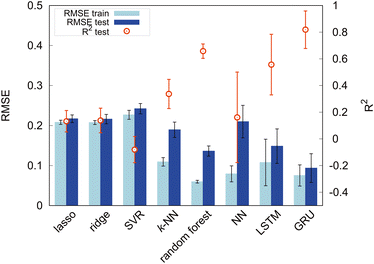
First, we set the modified-SMILES as the explanatory variable and evaluated the model performance, as shown in Fig. 6. The modified-SMILES considers the hydrophilicity and hydrophobicity of the molecules as well as the branching structures and the presence of cyclic arrangements in detail, thus serving as an exhaustive representation of the molecular structure. Consequently, using the modified-SMILES as the sole explanatory variable facilitates accurate predictions by the machine learning models. The results demonstrate that the random forest, LSTM, and GRU have relatively high performance, as shown in Fig. 6. The high performance of the LSTM and GRU models, in contrast to their machine learning counterparts, is attributed to the intrinsic characteristics of the modified-SMILES as sequence data, in which the order and presence of symbols are used to represent differences in molecular structures. Except for RNN algorithms, the order of data is not suggestive for predictions as a previous study has already shown that the accuracy of random forest before and after the permutation of data does not change much.²¹ Therefore, RNN algorithms are considered suitable for sequential data, such as molecular structure data. However, compared to RNN algorithms that require large amounts of data to create a decent model, random forest can be a good choice for a system with a relatively small amount of data, such as the present study with 305 data points.

Fig. 6 Comparison of model performance using the modified-SMILES as explanatory variables, with both the RMSE and model coefficient of determination (R²) being shown. Error bars represent the standard deviation.

Certain methods show high prediction accuracy but can be improved further. Therefore, in addition to the modified-SMILES direct molecular structure representation, we incorporate the frequency of k-mer tokens that represent the relative positional sense of different models. Generally, a k-mer denotes a contiguous substring of length k, and it is often used to represent and analyze sequential data such as DNA and amino acid sequences.^47,48 In this study, k-mers with k = 1, 2 are used because our models contain branching and ring structures; consequently, we may not be able to capture structures properly for k ≥ 3. In this study, k-mers with k = 1 correspond to particle types (T, H), and k-mers with k = 2 represent combinations of adjacent particles (T–T, T–H, H–H) signifying distinct bond types. In addition to the counts of pure k-mer tokens, we summed them and calculated their fraction. k = 1 k-mers represent the number of each particle; therefore, their sum is the overall number of particles in a molecule. The sum of k = 2 k-mers represents the overall number of bonds, and it should reflect the molecular structure in terms of the number of branches and cyclic structures. Self-assembly should also be affected by the ratio of particles or bonds against overall structures, as shown in Fig. 5; therefore, we calculated the fraction of k-mers by dividing the count of each k-mer by its sum. Thus, this study incorporates various explanatory variables, including the counts of k-mers for k = 1 and k = 2 as well as their sums and fractions against the overall structure. The above k-mer derived data were incorporated in the modified-SMILES implicitly; however, for a system with a small amount of data, such information may help to construct a better model to predict the self-assembly structures. Therefore, we used the k-mer derived data in conjunction with modified-SMILES representations in various machine learning algorithms to evaluate the effect. The assessment of model performance is shown in Fig. 7. A comparison of R² scores across models such as the random forest, LSTM, and GRU reveals that models that derive molecular structure insights using the modified-SMILES have comparatively higher prediction accuracy. Moreover, across all machine learning models, the model performance of the modified-SMILES augmented with k-mer information was superior to that of the modified-SMILES alone. This result highlights the relationship between k-mer information and molecular structure insights derived using the modified-SMILES. In conclusion, the combined use of the modified-SMILES and extracted particle and bond information is an effective approach for predicting molecular structures and elucidating their properties. This study reveals the importance of integrating diverse data sources to enhance the accuracy of predictive models.

Fig. 7 Comparison of model performance with explanatory variables set to the modified-SMILES and supplementary values, with both the RMSE and model coefficient of determination (R²) being shown. Error bars represent the standard deviation.

3.3 Machine learning analysis

We evaluate the factors influencing the self-assembly structure determination. First, the explanatory variables inputted are analyzed based on the feature importance derived from the high-performance random forest in this study. The feature importance, shown in Fig. 8, quantifies the contribution of each explanatory variable to random forest predictions. The introduced k-mer variables clearly play a significant role in predictions. The sum of k = 1 k-mers, representing the number of particles, and the sum of k = 2 k-mers, representing the number of bonds, exhibited relatively low feature importance, and the counts of k-mers for k = 1 and k = 2 showed feature importance equivalent to the SMILES. Moreover, the fractions of k = 1 k-mers, indicating the ratios of hydrophilic and hydrophobic particle components, dominantly contribute to the predictions, underscoring their key role in self-assembly structure determination. Although the increased feature importance suggests that the ratio of hydrophilic to hydrophobic particles dictates the self-assembly structure, Fig. 5 has already shown the inability to predict self-assembly structures accurately based solely on the hydrophilic component ratio. This underscores the complementary roles played by each explanatory variable, indicating that diverse interrelated factors determine the self-assembly structure of amphiphilic molecules. Among these, the proportion of hydrophilic and hydrophobic components within the molecule, essentially the amphiphilic nature, significantly influences the self-assembly structure of amphiphilic molecules.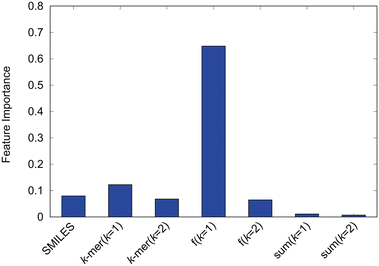

Fig. 8 Feature importance of the random forest model with the modified-SMILES and supplementary values as explanatory variables.

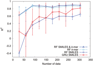
Next, to clarify the importance of the k-mer explanatory variables, we investigate the sample size dependence of the prediction accuracy. The sample size dependence of the prediction accuracy is illustrated in Fig. 9 for cases in which the modified-SMILES and k-mer values were used as explanatory variables and in which only the modified-SMILES or only the k-mer was used as an explanatory variable. With regard to random forest, incorporating k-mer values as explanatory variables clearly yields higher prediction accuracy across all sample sizes. When k-mer values are included as explanatory variables, high prediction accuracy is maintained even with smaller sample sizes, and reliable predictions can be achieved with sample sizes of around 80. This highlights the significance of k-mer explanatory variables and their key role in governing self-assembly structure determination. This fact becomes evident when comparing the sample size dependency when using the modified-SMILES and k-mer as explanatory variables versus using only the k-mer as the explanatory variable. In the case of random forest, incorporating the k-mer as an explanatory variable enhances the prediction accuracy.

Fig. 9 Sample size dependence of R² for four models: random forest and GRU with the modified-SMILES as an explanatory variable, random forest (RF) with supplementary values as explanatory variables, and random forest with the modified-SMILES and supplementary values as explanatory variables.

Next, we consider the sample size dependence of the GRU model employing only the modified-SMILES as the explanatory variable. With a sample size of 300, this model shows a prediction accuracy equivalent to that of the random forest model using the modified-SMILES and k-mer as explanatory variables. This implies that the GRU can learn the fundamental factors determining self-assembly structures, such as the amphiphilic nature of molecules and molecular structural characteristics, and directly predict self-assembly structures from the modified-SMILES alone without requiring k-mer explanatory variables. This result suggests the potential for extending GRU-based self-assembly structure predictions to general molecular structures, not limited to coarse-grained molecules, by using the general SMILES. The lack of a need to select and include auxiliary explanatory variables as additional inputs highlights the potential of extending the predictions not only to self-assembly structures but also to various other properties. However, when extending to general molecular structures, the sample size must be increased. Similar to the prediction results presented in Fig. 9 for the coarse-grained molecular model, increased sample sizes can improve the prediction accuracy. Furthermore, for extending to finer-grained general molecular structures, the sample size must be increased substantially. Although our focus here has been on the GRU, similar trends can be expected for LSTM, since both algorithms are derived from RNNs.

In summary, the representation method of molecular structures used as explanatory variables must be selected appropriately depending on the algorithm employed. The GRU directly inputs the SMILES molecular structure representation by learning the hydrophobicity of molecules and features of molecular structures, leading to highly accurate predictions. By contrast, random forest cannot capture the fundamental factors determining self-assembly structures from the SMILES; thus, molecular structures should be represented using k-mer tokens and be input as explanatory variables.

4 Conclusions

We used molecular simulations and machine learning to investigate the relationship between the molecular structure of amphiphilic parent molecules and their self-assembly behavior. We modeled various molecular structures, including not only linear structures but also branching and cyclic structures, and reproduced their self-assembly structures through molecular simulations. To characterize self-assembly structures, the CPP was used as a defining value. CPPs were calculated for all reproduced self-assembly structures in the simulations. The calculated CPPs agree with the actual self-assembly structures, thus serving as a useful index for evaluating the self-assembly structures. Furthermore, factors influencing self-assembly structures, such as the proportion of hydrophilic groups, were considered, and they exhibited strong correlations. However, obtaining self-assembly structures (CPPs) from molecular structures based only on these factors was challenging. Therefore, machine learning was used to predict the CPPs and to analyze the factors influencing them.

The molecular structures were described using the modified-SMILES as descriptors and explanatory variables as inputs. When using only the modified-SMILES for machine learning, the GRU showed the highest prediction accuracy, followed by random forest and LSTM, which also had strong performance. Subsequently, incorporating the k-mer into the machine learning process improved the prediction accuracy of all algorithms. Moreover, feature importance analysis and sample size dependence revealed that the amphiphilicity of molecules most strongly influences self-assembly structures. Considering that the efficiency of learning this information depends on the combination of algorithms and input data, the choice of an appropriate molecular structure representation method is crucial for each algorithm.

Though the self-assembly structure is known to change depending on the temperature and concentration of the system,⁴⁹ both values were maintained as constants in this study. Thus, our future study will aim to create models that can handle variations in these parameters. Lastly, the results suggest that using RNNs enables accurate predictions of self-assembly structures using only the SMILES, thus highlighting the potential for extending the predictions of various material properties of amphiphilic molecules. For systems with a small amount of data, using the random forest algorithm with a scalar quantity such as k-mer tokens improves the prediction. Overall, the study results show promise for significantly contributing to the molecular design of functional materials in the field of materials science.

Conflicts of interest

There are no conflicts of interest to declare.

References

1. D. Lombardo, M. A. Kiselev, S. Magazù and P. Calandra, Adv. Condens. Matter Phys., 2015, 151683.
2. W. Yan, W. Ning, L. Hao, C. Rukun, G. Jianmin, S. Ruibo, Z. Yongqiang, G. Lei, F. Xiaoyong and L. Donglin, J. Colloid Interface Sci., 2023, 629, 916–925.
3. P. Ambika and B. Amitabha, J. Cleaner Prod., 2017, 150, 127–134.
4. C. Shuo, H. Sara, F. James, L. Michelle and W. Jingyuan, Eur. J. Pharm. Biopharm., 2019, 144, 18–39.
5. V. Gunjan and P. A. Hassan, Phys. Chem. Chem. Phys., 2013, 15, 17016–17028.
6. X. Hu, R. Liu, D. Zhang, J. Zhang, Z. Li and Y. Luan, ACS Biomater. Sci. Eng., 2018, 4, 973–980.
7. D. Zhengyu, Q. Yinfeng, Y. Yongqiang, L. Guhuan, H. Jinming, Z. Guoying and L. Shiyong, J. Am. Chem. Soc., 2016, 138, 10452–10466.
8. R. V. D. Meel, M. H. A. M. Fens, P. Vader, W. W. van Solinge, O. E. Adefeso and R. M. Schiffelers, J. Controlled Release, 2014, 195, 72–85.
9. X. Cao, W. Guo, Q. Zhu, H. Ge, H. Yang, Y. Ke, X. Shi, X. Lu, Y. Feng and H. Yin, J. Colloid Interface Sci., 2023, 649, 403–415.
10. Z. Chu, C. A. Dreiss and Y. Feng, Chem. Soc. Rev., 2013, 42, 7174–7203.
11. H. T. Tien, R. H. Barish, L.-Q. Gu and A. L. Ottova, Anal. Sci., 1998, 14, 3–18.
12. Q. Ming, L. Tuo, H. Jirui, L. Zhichang, Y. Erlong and L. Xingquan, J. Pet. Sci. Eng., 2022, 208, 109695.
13. J. N. Israelachvili, Intermolecular and Surface Forces, Academic Press, 3rd edn, 2011.
14. A. L. Ferguson, J. Phys.: Condens. Matter, 2018, 30, 043002.
15. P. Friederich, A. Fediai, S. Kaiser, M. Konrad, N. Jung and W. Wenzel, Adv. Mater., 2019, 31, 1808256.
16. J. Kadupitiya, F. Sun, G. Fox and V. Jadhao, J. Comput. Sci., 2020, 42, 101107.
17. T. Terao, Soft Mater., 2020, 18, 215–227.
18. C. Kim, R. Batra, L. Chen, H. Tran and R. Ramprasad, Comput. Mater. Sci., 2021, 186, 110067.
19. R. A. Patel, C. H. Borca and M. A. Webb, Mol. Syst. Des. Eng., 2022, 7, 661–676.
20. T. Inokuchi, N. Li, K. Morohoshi and N. Arai, Nanoscale, 2018, 10, 16013.
21. D. Bhattacharya, D. C. Kleeblatt, A. Statt and W. F. Reinhart, Soft Matter, 2022, 18, 5037.
22. M. A. Webb, N. E. Jackson, P. S. Gil and J. J. de Pablo, Sci. Adv., 2020, 6, eabc6216.
23. P. J. Hoogerbrugge and J. M. V. A. Koelman, Europhys. Lett., 1992, 19, 155.
24. P. Espanol and P. Warren, Europhys. Lett., 1995, 30, 191.
25. R. D. Groot and P. B. Warren, J. Chem. Phys., 1997, 107, 4423–4435.
26. K. P. Santo and A. V. Neimark, Adv. Colloid Interface Sci., 2021, 298, 102545.
27. T. Yokoyama, H. Miwake, M. Hamaguchi, R. Nakatake and N. Arai, Mol. Syst. Des. Eng., 2023, 8, 538–550.
28. N. Arai, K. Yausoka and X. C. Zeng, J. Chem. Theory Comput., 2013, 9, 179–187.
29. R. D. Groot and T. J. Madden, J. Chem. Phys., 1998, 108, 8713–8724.
30. R. D. Groot and K. L. Rabone, Biophys. J., 2001, 81, 725–736.
31. P. Fabian, V. Gaeel, G. Alexandre, M. Vincent, T. Bertrand, G. Olivier, B. Mathieu, P. Peter, W. Ron, D. Vincent, V. Jake, P. Alexandre, C. David, B. Matthieu, P. Matthieu and D. Edouard, J. Mach. Learn. Res., 2011, 12, 2825–2830.
32. A. Paszke, S. Gross, F. Massa, A. Lerer, J. Bradbury, G. Chanan, T. Killeen, Z. Lin, N. Gimelshein, L. Antiga, A. Desmaison, A. Köpf, E. Yang, Z. D. Vito, M. Raison, A. Tejani, S. Chilamkurthy, B. Steiner, L. Fang, J. Bai and S. Chintala, Advances in neural information processing systems, 2019, vol. 32, pp. 8026–8037.
33. D. Weininger, J. Chem. Inf. Comput. Sci., 1988, 28, 31–36.
34. D. Weininger, A. Weininger and J. L. Weiningerr, J. Chem. Inf. Comput. Sci., 1989, 29, 97–101.
35. D. Weininger, J. Chem. Inf. Comput. Sci., 1990, 30, 237–243.
36. Y. Mai and A. Eisenberg, Chem. Soc. Rev., 2012, 41, 5969–5985.
37. N. A. Lynd, A. J. Meuler and M. A. Hillmyer, Prog. Polym. Sci., 2008, 33, 875–893.
38. T. Robert, J. R. Stat. Soc., Ser. B, Methodol., 1996, 58, 267–288.
39. A. E. Hoerl and R. W. Kennard, Technometrics, 1970, 12, 55–67.
40. A. E. Hoerl and R. W. Kennard, Technometrics, 1970, 12, 69–82.
41. E. Fix and J. L. Hodges, Int. Stat. Rev., 1989, 57, 238–247.
42. H. Drucker, C. J. Burges, L. Kaufman, A. Smola and V. Vapoik, Advances in Neural Information Processing Systems, 1997, vol. 9, pp. 155–161.
43. B. Leo, Mach. Learn., 2001, 45, 4–32.
44. L. F. Scabini and O. M. Bruno, Phys. A, 2023, 615, 128585.
45. S. Hochreiter and J. Schmidhuber, Neural Comput., 1997, 9, 1735–1780.
46. K. Cho, B. van Merrienboer, C. Gulcehre, D. Bahdanau, F. Bougares, H. Schwenk and Y. Bengio, Proceedings of the 2014 Conference on Empirical Methods in Natural Language Processing (EMNLP), 2014, pp. 1724–1734.
47. A. Rahman, I. Hallgrimsdottir, M. Eisen and L. Pachter, eLife, 2018, 7, e32920.
48. E. Asgari, K. Garakani, A. C. McHardy and M. R. K. Mofrad, Bioinformatics, 2018, 34, i32–i42.
49. A. Bernheim-Groswasser, E. Wachtel and Y. Talmon, Langmuir, 2000, 16, 4131–4140.

---