DOI:
10.1039/D4SM01426J
(Paper)
Soft Matter, 2025,
21, 2586-2606
Spontaneous generation of angular momentum in chiral active crystals
Received
1st December 2024
, Accepted 21st February 2025
First published on 26th February 2025
Abstract
We study a two-dimensional chiral active crystal composed of underdamped chiral active particles. These particles, characterized by intrinsic handedness and persistence, interact via linear forces derived from harmonic potentials. Chirality plays a pivotal role in shaping the system's behavior: it reduces displacement and velocity fluctuations while inducing cross-spatial correlations among different Cartesian components of velocity. These features distinguish chiral crystals from their non-chiral counterparts, leading to the emergence of net angular momentum, as predicted analytically. This angular momentum, driven by the torque generated by the chiral active force, exhibits a non-monotonic dependence on the degree of chirality. Additionally, it contributes to the entropy production rate, as revealed through a path-integral analysis. We investigate the dynamic properties of the crystal in both Fourier and real space. Chirality induces a non-dispersive peak in the displacement spectrum, which underlies the generation of angular momentum and oscillations in time-dependent autocorrelation functions or mean-square displacement, all of which are analytically predicted.
Introduction
The term “chirality”, derived from the ancient Greek word “χειρ” meaning “hand”, was coined by Lord Kelvin in 1873 to describe the property of an object that cannot be superimposed onto its mirror image.1 Chirality, also known as handedness, refers to the characteristic of being either right-handed or left-handed. This property is observed across various scales in nature, from organic molecules like DNA and proteins to different organisms such as plants and animals. For instance, snails exhibit chirality, with some possessing right-handed spiraling shells while others have left-handed shells or spiral in a clockwise/counterclockwise direction.2 Chirality is also evident in the spiral arrangement of leaves, stems, roots, and floral parts in plants.
Chirality has found applications in active matter,3–5 where materials are engineered to exhibit specific behaviors, offering opportunities for designing structures with diverse functionalities. As a result, there has been increasing interest in studying the behavior of chiral self-propelled particles,6,7 both synthetic and natural, to achieve control over their motion. These particles exhibit two distinctive properties: first, they break time-reversal symmetry, converting energy into directed motion and dissipated heat; second, they break reflection symmetry, inherently existing far from equilibrium. The breaking of time-reversal symmetry gives rise to phenomena absent in equilibrium systems, such as flocking,8,9 motility-induced phase separation,10–14 spatial velocity correlations,15–20 and accumulation near obstacles.21–24 In contrast, the breaking of reflection symmetry results in distinct phenomena, including odd diffusivity25–27 and odd viscosity.28–31 A prominent example of broken parity is the Hall effect, where moving charges in a conductor subjected to a magnetic field produce an electric potential difference perpendicular to both the motion and the field, manifesting as an off-diagonal Hall resistance. Focusing on active matter, numerous examples of chirality are found in both natural systems and synthetic structures. Observing circular swimming in two dimensions or helical swimming in three dimensions requires only a slight asymmetry in the active particles relative to their propulsion axis32,33 or the presence of an external magnetic field.34 For instance, magnetotactic bacteria, which are motile prokaryotes equipped with magnetosome organelles, act like miniature compasses, swimming along magnetic field lines. In addition, droplets of cholesteric liquid crystals in isotropic liquids35 and artificial self-propelled L-shaped particles32 also display circular trajectories. Examples of chiral systems exist also at the macroscopic scale where inertia plays a fundamental role. This is the case of chiral active particles, such as vibrobots or spinners which self-rotate and show circular motion.36–39
The behavior of individual chiral active particles is well understood: the angular drift leads to circular trajectories40 (see Fig. 1(a)), resulting in temporal oscillations in velocity autocorrelations and mean-square displacement, as well as a reduction in long-time diffusion.29,40–46 Beyond the case of a potential-free particle, the role of chirality has been investigated in various scenarios: dimers composed of two chiral particles,47 harmonic confinement where chirality reduces the effective temperature induced by activity,48 and near planar obstacles where circular motion mitigates the wall accumulation typically observed in active particles.49–52
 |
| | Fig. 1 Chiral active crystals. (a) Illustration of a chiral active particles which self-propel (red arrow) and rotate counterclockwise (blue arrow) performing a circular trajectory. (b) Illustration of a chiral active crystal in two dimensions in a triangular lattice. Chirality induces rotating modes (a non-dispersive peak in the displacement spectrum) which generates a global angular momentum. | |
Moreover, the impact of chirality on collective phenomena has been extensively investigated, both in the presence and absence of alignment mechanisms. In systems with alignment interactions, chirality gives rise to pattern formation,53–64 including phenomena such as chiral self-recognition,65 traveling waves,66 and rotating micro-flock patterns.53 In the absence of alignment interactions, chirality suppresses motility-induced phase separation67–71 and induces a hyperuniform phase.72–76 Additionally, circular motion reduces spatial velocity correlations by decreasing their correlation length.77 In this case, chirality appears to primarily diminish the distinctive effects characteristic of active matter. However, recent studies have highlighted novel phenomena that are primarily associated with rotational dynamics arising from circular motion. These effects include unique oscillatory caging phenomena in chiral active glasses,78 fascinating vortex patterns in velocity fields,67,79 self-reverting vorticity in the presence of attractive interactions,80 and demixing in binary mixtures.81–83
Understanding the role of activity and chirality in active crystals remains a challenge. In the absence of lattice vacancies, the particles in a solid structure are restricted to vibrate around their lattice positions rather than diffuse. In one- and two-dimensional systems, these vibrational excursions can be substantial, even diverging for infinite systems. While the physics of non-chiral solids has been extensively studied, the inclusion of chirality introduces additional complexity. Recently, this problem was addressed by Shee et al.,77 who employed a continuum theory. Their study predicts that chiral active crystals exhibit spatial velocity correlations following an Ornstein–Zernike profile, as seen in non-chiral active solids,16,84,85 with a correlation length that decreases as chirality increases.
In our paper, we investigate chiral active crystals using a particle-based approach, previously applied to non-chiral crystals86 (see Fig. 1(b) for an illustration). Motivated by macroscopic experimental systems, such as active granular particles, we consider chiral active dynamics in the underdamped regime. This general treatment includes the overdamped motion typical of chiral colloids as the subcase with vanishing inertia. For harmonic crystals, our theoretical method enables us to analytically derive the displacement spectrum without the need for parameter fitting, as well as to make approximations for predicting spatiotemporal correlations in real space. After validating the findings of ref. 77 on spatial velocity correlations, we discover that chirality induces spatial structures in the cross-velocity correlations, involving mixed Cartesian components. This phenomenon is associated with a net angular momentum entirely driven by circular motion, which displays a non-monotonic dependence on chirality. The analytical solution for the displacement spectrum reveals the presence of a non-dispersive peak at the chirality frequency, which underpins temporal oscillations in displacement autocorrelations and mean-square displacements. Interestingly, chirality introduces an additional contribution to entropy production, arising from the torque exerted by the active forces on the particles of the crystal.
The paper is organized as follows: Section 2 introduces the model, presenting an extension of the active Ornstein–Uhlenbeck model to describe a two-dimensional chiral active crystal. Section 3 examines the model's dynamical correlations in the frequency and wave vector domains, including displacement correlations (both diagonal and off-diagonal) and angular momentum. In Section 4, we analyze the steady-state properties of the system, such as equal-time displacement–displacement and velocity–velocity correlations, angular momentum, and entropy production, while in Section 5 we explore the system's temporal behavior, including the mean-square displacement and the two-time correlations of velocity and displacement. Finally, Section 6 presents the conclusions. The paper also includes several appendices that detail technical aspects omitted from the main text for clarity and brevity.
Model for chiral active crystals
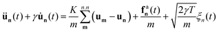
We consider a two-dimensional non-equilibrium crystal composed of chiral active particles in the underdamped regime. This choice is motivated by the existence of macroscopic chiral active matter systems where inertia is not negligible. In addition, the overdamped case typical of chiral active colloids can be easily recovered by taking the limit of vanishing mass. Each particle is harmonically connected to its neighbors and subjected to an additional chiral active force that induces clockwise or counterclockwise rotations. Specifically, the particles are distinguishable and labeled by a two-dimensional index n = (n1,n2). They oscillate around their equilibrium lattice positions, Rn, under the influence of random, active, and conservative forces governing their dynamics. The instantaneous coordinates rn(t) of the particles are described by the following set of coupled Langevin equations:| |  | (1) |
where ζn(t) is a white noise with zero mean and unit variance. The term γ is a friction coefficient per unit mass, such that the inertial time is simply 1/γ. The constant T sets the amplitude of the noise, which corresponds to the solvent temperature in the case of active colloids or it is generated by plate and particle imperfections in active granular particles.87 The term  represents the conservative force at position rn arising from a potential U ensuring that the particle is maintained at the lattice spacing σ. Assuming short-range interactions, the sum
  is taken over the nearest neighbors of the particle which at equilibrium occupies the lattice position, Rn. The term fan represents the active or self-propelled force driving each particle out of equilibrium. The evolution of fan follows the active Ornstein–Uhlenbeck particle (AOUP) dynamics88–90 extended to include chirality,49 and is expressed as
| |  | (2) |
where χn(t) is a white noise with zero mean and unit variance.
The terms v0 and τ represent the typical particle speed and the persistence time, respectively, i.e. the time required for a particle to randomize its velocity. Following ref. 49, chirality is incorporated into the dynamics by introducing the term Ω × fan, where Ω = Ωz is a vector perpendicular to the plane of motion with a magnitude of Ω (z is the unit vector in the vertical direction). The parameter Ω is an effective constant torque and is commonly referred to as chirality, determining the revolution time of fan. This model can be interpreted as a Gaussian approximation of chiral active Brownian motion. It reproduces the temporal correlation functions of fan in the steady state, expressed as follows:
| |  | (3a) |
| |  | (3b) |
| |  | (3c) |
where

. The active forces act independently on different particles, as shown by the presence of the Kronecker symbols. As is typical for non-chiral active particles, the persistence time
τ corresponds to the decay time of the temporal autocorrelations. Chirality introduces two primary effects:
(i) It induces oscillations with frequency Ω and (ii) gives rise to cross-temporal correlations, i.e., correlations between different Cartesian components of the active force. These cross-correlations vanish as Ω → 0 and exhibit odd symmetry under the exchange of x and y, as evident from eqn (3c). This property underpins the odd diffusivity, an antisymmetric diffusion tensor, which has been previously predicted for chiral active particles.25 Notice that the active force is subject to an overdamped dynamics because in experiments of inertial active matter, such as active granular particles,91 rotational inertia is often negligible.
Assuming harmonic interactions among nearest neighbor particles and introducing the displacement un with respect to their equilibrium position as un = rn − Rn, we focus on the dynamics of the displacement vectors
| |  | (4) |
where
K is the strength of the elastic restoring force. In the case of a non-linear potential
K can be determined by differentiating the potential
U(
r), such that
K =
U′′(
σ) +
U′(
σ)/
σ, where
σ is the lattice spacing.
Dynamical correlations
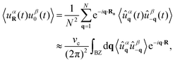
The dynamics (4) can be solved by switching to normal coordinates and applying the double Fourier-transform of the variables moving from the discrete space of coordinates indexed by n and the time domain t to the discrete wave vector q = (qx,qy) and frequency ω. Specifically, we use the continuum Fourier transform to handle the time domain and the discrete Fourier transform for the spatial coordinates. In this way, we obtain| |  | (5) |
where the double Fourier transforms of any variables are indicated by a ‘tilde’ symbol and by the explicit dependence on q and ω. The same definition can be applied to the velocity, active force, and noise variables. In addition, a ‘hat’ symbol denotes the spatial Fourier transform of a variable and a ‘bar’ symbol the Fourier transform in frequency (see Appendix A). Since the velocity variable is given  , its double Fourier transform satisfies the relation ṽq(ω) = iωũq(ω). By applying the time and space Fourier transform to eqn (4), we obtain the evolution of each Fourier mode of the displacement
| | 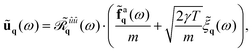 | (6) |
where we have introduced the matrix ![[scr R, script letter R]](https://www.rsc.org/images/entities/char_e531.gif) ũũq(ω)) = Gq(ω)I written as the product between the identiy matrix I and the propagator
ũũq(ω)) = Gq(ω)I written as the product between the identiy matrix I and the propagator ![[G with combining tilde]](https://www.rsc.org/images/entities/i_char_0047_0303.gif) q(ω) given by q(ω) = (−ω2 + iωγ + ωq2)−1. Here, ωq is the frequency of the vibrational modes of the crystal, which for a triangular lattice with lattice constant σ, reads:
q(ω) given by q(ω) = (−ω2 + iωγ + ωq2)−1. Here, ωq is the frequency of the vibrational modes of the crystal, which for a triangular lattice with lattice constant σ, reads:| | 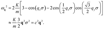 | (7) |
In the last approximation, we have expanded ωq for small wave vectors q, obtaining the usual q2 behavior and we have introduced c, as the equivalent of the speed of sound.
Dynamical correlations of the particle displacement
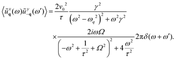
From the explicit solution (6), the displacement correlation functions in the (q,ω) representation can be readily derived by utilizing the correlation properties of the noise. The detailed calculations are provided in Appendix B, but here we present the expression for the dynamical correlations of the particle displacement with the same Cartesian index:| | 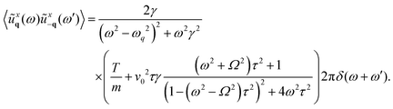 | (8) |
For harmonic interactions, we observe an invariance for along x and y, or in other words we have 〈ũyq(ω)ũy−q(−ω)〉 = 〈ũxq(ω)ũx−q(−ω)〉. The expression for 〈ũxq(ω)ũx−q(−ω)〉 consists of two terms: (i) a thermal contribution related to equilibrium phonons and (ii) a non-equilibrium, active contribution with a different functional form. (i) Corresponds with the first term within the parentheses in eqn (8) and accounts for the displacement correlation stemming from thermal fluctuations in the presence of dissipative dynamics. The amplitude of this equilibrium term is determined by the constant temperature T. As is typical in equilibrium systems, the inertial term 1/γ governs a transition between monotonic decay and damped oscillatory behavior. Specifically, for wavevectors satisfying ωq2 > γ2/4, the poles of ûûq(ω) are complex (underdamped regime), while for ωq2 < γ2/4 the poles become purely imaginary (overdamped regime). This implies that in the underdamped regime dispersive phononic peaks at ω = ±ωq are expected (Fig. 2(a)–(d)). In the overdamped regime, however, a single peak at ω = 0 emerges (Fig. 2(e)–(h)). The term (ii) represents a non-equilibrium contribution arising from the active force with its amplitude determined by the so-called active temperature, defined here as v02τγ. Although this term exhibits the same wave vector dependence as the thermal contribution, the non-equilibrium contribution is characterized by a prefactor that explicit depends on the frequency ω (see the second term in the parentheses in eqn (8)). Whether this frequency-dependent term can be interpreted as an effective temperature lies beyond the scope of this work. While this frequency-dependent prefactor includes an explicit dependence on the persistence time τ, as noted previously,86,92 we emphasize here that its value is significantly influenced by the chirality Ω. In the absence of chirality Ω, the prefactor simplifies to 1/(1 + ω2τ2), which is a function peaked at ω = 0. In contrast, when Ω > 0, the prefactor is peaked at the frequency ω = Ω.
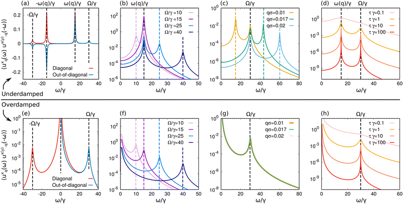 |
| | Fig. 2 Dynamical correlation of the displacement. (a) and (e) Diagonal correlations of the particle displacement (normalized with the lattice constant σ), 〈uxq(ω)ux−q(−ω)〉 (red) and imaginary part of the out-of-diagonal correlations of the particle displacement 〈uxq(ω)uy−q(−ω)〉 (blue). These observables are plotted as a function of the frequency ω rescaled with the inertial time 1/γ at wave number modulus q = |q|. (b) and (f) 〈uxq(ω)ux−q(−ω)〉 for different chirality values Ω/γ. (c) and (g) 〈uxq(ω)ux−q(−ω)〉 for different rescaled wave numbers q = |q|. (d) and (h) 〈uxq(ω)ux−q(−ω)〉 for different persistence time τγ. (a)–(d) Are obtained with K/(γ2m) = 105, while (e)–(h) are obtained with K/(γ2m) = 103. In all the panels, vertical dashed lines are used to denote the peak frequencies, i.e. Ω/γ and when it is not explicitly stated, the curves are obtained with q = |q| = 10−2, Ω/γ = 30, mv02/T = 102, and τγ = 2. | |
In Fig. 2(a) and (e), the displacement correlations 〈ũxq(ω)ũx−q(−ω)〉 are shown as a function of the frequency ω at fixed wave vector q. In the underdamped regime (Fig. 2(a)), the dynamical correlations are characterized by four peaks. Two of these peaks occur at the phonon frequencies ω ± ωq and are driven by both the thermal and non-equilibrium contributions described in eqn (8); these peaks are only weakly influenced on the chirality Ω which does not alter their positions and are not present in the overdamped regime (Fig. 2(e)) where 〈ũxq(ω)ũx−q(−ω)〉 has a single peak in the origin. The two additional peaks, present in both the underdamped and overdamped regimes, are entirely induced by activity, particularly by chirality. These peaks occur at frequencies ω = −±Ω (Fig. 2(b) and (f)) and collapse to the origin as Ω → 0. Notably, these are non-dispersive peaks, as their positions do not depend on the wave vector q (Fig. 2(c) and (g)), in contrast to the peaks at ω = ±ωq, whose positions are determined by the relation ωq2 ∼ Kq2. Finally, the persistence time τ does not influence the positions of the peaks but rather affects their widths and heights. Specifically, larger values of τ result in narrower and taller peaks (Fig. 2(d) and (h)). Consequently, we conclude that the persistence time has a dynamical effect analogous to inertia, while chirality can produce non-dispersive peaks at the frequency determined by the angular velocity Ω. Since these effects and the influence of chirality arise in both overdamped and underdamped regimes, we will, in the following, evaluate static correlation functions exclusively in the overdamped case, where analytical results can be explicitly obtained.
Spectral density of cross correlation and angular momentum
One of the most distinctive traits of the chiral model is the existence of cross-correlations, meaning the x component of displacement (or velocity) exhibits a non-zero correlation with its y component. Moreover, swapping the components results in a change in the sign of the correlation: 〈ũyq(ω)ũx−q(−ω)〉 = −〈ũxq(ω)ũy−q(−ω)〉. Specifically, the cross ω-correlations are purely imaginary, arising solely from active fluctuations and remaining unaffected by thermal noise:| | 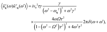 | (9) |
where i is the imaginary unit. This expression is evaluated in Appendix B. The imaginary part of these cross-correlations qualitatively resembles the diagonal dynamical correlations of the displacement. Both types of correlations exhibit the same peaks, at ω = ±ωq2 and ω = ±Ω as well as the same parameter dependencies (Fig. 2(a)). However, 〈ũxq(ω)ũy−q(−ω)〉 is an odd function of ω and Ω and contains no thermal contributions. The amplitude of this correlation is solely determined by the active temperature v02γτ. The presence of non-vanishing cross-correlations in particle displacement leads to a non-zero spectral density of angular momentum, M. This quantity is defined as the dynamical correlations between the cross-product of displacement and velocity. It serves as a measure of how the signal varies across a given frequency and wavevector, enabling the isolation of contributions from various length scales and timescales. By employing the solution (6) and recalling that ṽq(ω) = iωũq(ω), we derive (see Appendix B):| |  | (10) |
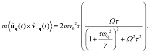
where ẑ represents the unit vector along the vertical direction. In this expression, the ω-dependence of ![[M with combining tilde]](https://www.rsc.org/images/entities/b_char_004d_0303.gif) q(ω) closely resembles that of the displacement–displacement correlation function (9). Specifically, q(ω) and 〈ũxq(ω)ũy−q(−ω)〉 share the same denominator, leading to identical imaginary or complex poles. The key distinction lies in the ω2 dependence in the numerator of q(ω), which makes this function even with respect to ω. As a result, q(ω) exhibits two pairs of distinct peaks. The first pair occurs very near the phonon frequencies, ±ωq, while the second appears at a frequency close to the angular drift frequency, ±Ω. Similar to the dynamical correlation of the displacement, the latter peak is non-dispersive, meaning that the frequency of its maximum is nearly independent of the wavevector q. Furthermore, it is notable that the spectrum of the angular momentum remains independent of temperature, as it is driven solely by the active chiral noise. We anticipate that the even ω-dependence in eqn (10) indicates that a chiral active crystal will exhibit a non-zero total angular momentum. This property arises solely due to chirality, as the total angular momentum vanishes for non-chiral active or passive crystals. This idea will be explored further in the next section through explicit real-space calculations.
q(ω) closely resembles that of the displacement–displacement correlation function (9). Specifically, q(ω) and 〈ũxq(ω)ũy−q(−ω)〉 share the same denominator, leading to identical imaginary or complex poles. The key distinction lies in the ω2 dependence in the numerator of q(ω), which makes this function even with respect to ω. As a result, q(ω) exhibits two pairs of distinct peaks. The first pair occurs very near the phonon frequencies, ±ωq, while the second appears at a frequency close to the angular drift frequency, ±Ω. Similar to the dynamical correlation of the displacement, the latter peak is non-dispersive, meaning that the frequency of its maximum is nearly independent of the wavevector q. Furthermore, it is notable that the spectrum of the angular momentum remains independent of temperature, as it is driven solely by the active chiral noise. We anticipate that the even ω-dependence in eqn (10) indicates that a chiral active crystal will exhibit a non-zero total angular momentum. This property arises solely due to chirality, as the total angular momentum vanishes for non-chiral active or passive crystals. This idea will be explored further in the next section through explicit real-space calculations.
Cross-correlations and angular momentum are also at the basis of the edge currents typically observed in chiral active systems. This effect can be observed even for a single chiral particle in a flat channel or an external potential: when the particle is close to the wall, its rotating trajectory leads to a momentum flux tangential to the wall profile.49 The cross-correlations observed here suggest that a similar effect may occur in a two-dimensional chiral active crystal confined by a wall along one direction.
Spatial correlations
In this section, we will focus on the static correlation functions in the steady state, i.e. t → ∞. In principle, time correlations can be obtained from their ω-representation by analytically performing the necessary Fourier transforms through complex integration. This task becomes less demanding when considering the overdamped limit, where the propagator simplifies and becomes q(ω) = (iωγ + ωq2)−1. Moreover, in the previous section, we have discovered that chirality affects the displacement spectrum by introducing two symmetric peaks at the chiral frequency ω = ±Ω both in the underdamped and overdamped regimes. Since these peaks are not affected by inertia, we conclude that the choice of overdamped or underdamped regimes is irrelevant to understanding the role of chirality in active crystals. Therefore, in this section, we limit our theoretical treatment to the overdamped case.
The equal-time correlations can be derived by integrating the dynamical correlations, such as eqn (8) and (9), over the entire frequency range ω. For example, the displacement spatial correlations in the wave vector domain q at equal time are expressed as:
| |  | (11) |
where
α,
β =
x,
y. Since the dynamical cross-correlations are odd functions of the frequency
ω, the equal-time correlations 〈
ûxq(
t)
ûy−q(
t)〉 = 〈
ûyq(
t)
ûx−q(
t)〉 = 0 vanish in the steady state, as evident by considering the definition
(11).
This procedure can also be applied to other variables, such as velocity and self-propulsion to obtain general correlations of dynamical variables as a function of q. By performing the inverse q-Fourier transform in two dimensions, one can derive the real space profile of these correlations:
| |  | (12) |
where
R is a real-space vector identifying the particle position and in the last approximation, the sum over
q is replaced by an integral over the Brillouin region BZ. Here,
vc represents the volume of the unit (Wigner–Seitz) cell of the crystal. By evaluating
eqn (12) at
R = 0, we obtain the mean-square displacement.
For our convenience, rather than transforming the correlation functions from the ω domain to the time domain, we have adopted a different but equivalent strategy, detailed in Appendix C, which directly utilizes the time domain to evaluate the correlations. Using the methods outlined in Appendix C, the diagonal components of the equal-time displacement correlations are given by
| |  | (13) |
Similarly to the ω-correlations, the expression for 〈uxq(t)ux−q(t)〉 contains two terms derived from direct integration of the two contributions in eqn (8). The first term originates thermally and is proportional to the temperature of the thermal bath, while the second term is entirely induced by the activity (∝γτv02) and vanishes in the equilibrium limit v0 → 0. Consequently, the first term represents the standard passive contribution describing equilibrium dynamics, whereas the second introduces a novel source of fluctuations stemming from non-equilibrium effects. Both the thermal and active terms contain a factor 1/ωq2 which diverges as 1/q2 as q approaches 0. The active contribution contains an additional q-dependence through τωq2/γ, that indicates the presence of non-equilibrium correlations in the displacement spectrum, which qualitatively differ from those at equilibrium. These non-equilibrium displacement fluctuations are also present when chirality vanishes (Ω = 0) and diminish in amplitude as Ω2τ2 increases. The circular nature of the particles' trajectories reduces the spatial fluctuations of the displacements and effectively increases the stiffness of the spring constants. The effect of chirality, as shown by the structure of the second term in the equal-time pair correlation (13), is most amplified when q satisfies the condition τ < γ/ωq2. In fact, below a critical value qcrit, defined by the condition  , the active forces make a significant contribution to the correlations.
The mean square displacement of the particles from their equilibrium position is given by the expression:  , which upon converting the sums into integrals as in eqn (12), reads:
  , where the integral, in principle, extends to the first Brillouin zone (BZ). However, in practice, we employ the Debye continuum approximation, which assumes a linear dispersion relation ∼q up to a maximum frequency, the Debye frequency. In this way, the lattice is treated as a continuous elastic medium, with a cutoff wavevector to match the number of allowed vibrational modes to the actual number of the lattice degrees of freedom. The model has the advantage of being mathematically straightforward and computationally efficient: it provides a reasonable approximation for low-frequency (long-wavelength) acoustic phonons where the linear dispersion relation is valid.
Utilizing eqn (13) to perform the integral in polar coordinates, denoted as  , with qmin = 2π/Na and qD = π/a. Since the integral is peaked near q = 0, we approximate the last fraction in eqn (13) as (1 + Ω2τ2)−1 and use the small-q approximation for ωq2 ≈ 3K/(2m)q2σ2 = c2q2, and obtain:
| | 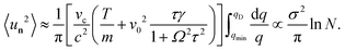 | (14) |
This logarithmic divergence for N → ∞ aligns with the Mermin–Wagner theorem predicting the absence of long-range translational order in a chiral active crystal. Both the thermal and active fluctuations suppress the long-range translational order. However, compared to the corresponding non-chiral active crystal, the amplitude of the displacement fluctuations described by eqn (14) decreases as the persistence time τ and the chirality Ω increase. This behavior is consistent with the fact that the diffusivity of freely moving chiral particles is smaller than the one on non-chiral particles. However, in more realistic situations where vacancies are present, the curvature of the trajectories induced by the chirality might favor the displacement of the particles (see Kalz et al.26)
On the other hand, the difference  between any pair of sites (n and n′) exhibits only finite fluctuations if their separation is finite, indicating that local order is preserved. Notably, in active chiral systems, both the mean square displacement and
  are reduced compared to their values in the achiral case. This reduction occurs because the trajectories in systems with chirality (Ω ≠ 0) are curved, and the positional fluctuations are reduced by activity. This behavior is consistent with the dynamics of an active particle in a harmonic potential.48 The particle number density can be expressed as the sum of delta functions positioned at rn(t),
  , where rn = Rn + un. Its Fourier transform, assuming 〈un〉 to be independent of the site index, reads:
 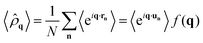 , where
  represents the Fourier transformed density of the frozen lattice. It is maximal when q = G, where G is a reciprocal wave-vector. Since the displacements have a Gaussian distribution, we write: 〈eiG·un〉 = e−〈(G·un)2〉/2 = e−WG. Thus, the Fourier components of the density associated with the reciprocal wave-vectors are 〈
![[small rho, Greek, circumflex]](https://www.rsc.org/images/entities/i_char_e0b7.gif) G〉 = f(G)e−WG with
G〉 = f(G)e−WG with  . Employing the approximate correlator and obtaining the following estimate:
| |  | (15) |
The Debye–Waller factor e−WG vanishes for large systems as L → ∞ (N → ∞), and for any G ≠ 0, 〈G〉 = f(G)e−WG → 0. The displacement u has infinite fluctuations, and the periodic order parameter, 〈G〉, is washed out. Only the amplitude corresponding to G = 0 remains finite in the infinite volume limit. However, unlike a liquid, the system displays power-law correlations.
Chirality effect on spatial velocity correlations
An active crystal, composed of self-propelled particles without alignment interactions, exhibits spatial structures in velocity correlations. This phenomenon manifests in the formation of spatial domains where particles share the same (correlated) velocity, a behavior referred to as spontaneous velocity alignment.15 This nonequilibrium collective effect has been observed in previous numerical studies, which predict an Ornstein–Zernike profile16,20,84,85 with a correlation length analytically derived in terms of the model parameters.17 This correlation length increases with the square root of the persistence time and grows linearly with the spring strength. Here, we evaluate the effect of chirality on spatial velocity correlations. The static velocity correlation can indeed be derived explicitly (see Appendix C) and is given by:| |  | (16) |
where the latter approximation holds in the limit of small wavevector q. Consequently, chirality does not modify the Ornstein–Zernike profile observed for non-chiral particles (Fig. 3(a)). As with displacement correlations, the velocity correlations, 〈vαq(t)vα−q(t)〉, comprise two distinct contributions: (i) an equilibrium term, which remains constant (∝T) and does not induce any spatial structure in the velocity field, and (ii) an active term, whose amplitude is governed by the swim velocity v02 and vanishes in the equilibrium limit v0 → 0. The active term introduces a wave vector dependence, and creates spatial correlations in the velocity field.
 |
| | Fig. 3 Chirality-suppressed spatial velocity correlations (a) and (b) spatial velocity correlations 〈vxqvx−q〉 (normalized by 〈vx0vx−0〉) as a function of the wave vector modulus q = |q| rescaled with the particle diameter σ. (a) Shows 〈vxqvx−q〉 for different values of the reduced chirality Ω/γ at fixed reduced inertia τγ = 1, while (b) shows m(q) for different τγ at fixed Ω/γ = 1. (c) Correlation length ξ of the spatial velocity correlations (normalized by correlation length calculated at zero chirality ξ(Ω = 0)) as a function of/for different values of τγ. In all the panels, the curves are obtained with mv02/T = 102 and K/(γ2m) = 103. | |
The role of chirality manifests in a faster decay, as shown at fixed τγ by varying the chirality parameter Ω/γ (Fig. 3(a)). The Ornstein–Zernike profile (16) allows us to introduce a correlation length ξ as ∼1/(1 + ξ2q2) which quantifies the size of the spatial domains where particle velocities are aligned. The length ξ decreases as Ωτ is increased (Fig. 3(c)) according to the formula:
| |  | (17) |
where
U′ and
U′′ denotes the first and second derivative of the potential evaluated at the lattice distance
σ.
Eqn (17) reproduces previous results
15,16,84 in the limit of vanishing chirality,
Ω = 0, and incorporates a chirality dependence consistent with the findings of ref.
77, which employed an alternative continuum approach. The decrease in
ξ arises because chirality induces rotational motion in the particle trajectories, with a radius that decreases as
Ω increases. This results in a smaller effective persistence length compared to the non-chiral case, leading to reduced spatial domains where velocities remain correlated. In addition, consistent with the non-chiral case, a strong potential and/or a large value of
τ (at fixed
Ω) lead to slower decays of the spatial velocity correlations (
Fig. 3(b)), which corresponds to a larger correlation length
ξ. By performing a Fourier transform of the profile in
eqn (16), it is found that the velocities exhibit exponentially decaying correlations in real space. An estimate of the long-distance behavior of the velocity correlation function is:
| |  | (18) |
Here, we have omitted a delta-like contribution arising from the passive term, as T ≪ v02γτ. In the first approximation, we took the continuum limit, replacing the summation over discrete wavevectors with an integral over the first Brillouin zone. In the second approximation, we evaluated the correlation at long distances, deriving the asymptotic behavior of the spatial velocity correlations.
Chirality-induced angular momentum
Chirality primarily manifests through circular trajectories and a propensity for rotational motion. Consequently, it is not surprising that spatial velocity correlations are insufficient for effectively capturing novel collective effects induced by chirality. To address this limitation, we propose using the angular momentum field93 as a steady-state observable to quantify the system's handedness. This observable can be determined by integrating the spectral density of the angular momentum (eqn (10)) over the frequency ω, or directly from the equal-time off-diagonal correlation between velocity and displacement, yielding:| |  | (19) |
Here, ẑ represents a unit vector in the vertical direction. In the final approximation, we have expanded ωq for small q, retaining only the leading order in q. Eqn (19) reveals that the angular momentum exhibits a q-dependence, indicating the presence of a steady-state spatial structure in real space. Specifically, mq follows an Ornstein–Zernike profile with a correlation length of 2ξ, where ξ is defined in eqn (17). This behavior is illustrated for different values of Ω (Fig. 4(a)) and different values of τ (Fig. 4(b)). Notably, the amplitude of |![[m with combining circumflex]](https://www.rsc.org/images/entities/b_char_006d_0302.gif) q=0| increases monotonically with τ, whereas it exhibits a non-monotonic dependence on Ω. This suggests that chirality may impart a non-monotonic effect on the total angular momentum M. This global observable is obtained by summing contributions mq from all modes q and normalizing by the number of particles N:
q=0| increases monotonically with τ, whereas it exhibits a non-monotonic dependence on Ω. This suggests that chirality may impart a non-monotonic effect on the total angular momentum M. This global observable is obtained by summing contributions mq from all modes q and normalizing by the number of particles N:
| |  | (20) |
 |
| | Fig. 4 Chirality-induced angular momentum. (a) and (b) Vertical component of the angular momentum mq = 〈uq × v−q〉 + c.c. = mqẑ as a function of wave vector modulus q = |q| rescaled with the particle diameter. (a) shows mq for different values of the reduced chirality Ω/γ at fixed reduced inertia τγ = 1, while (b) shows m(q) for different τγ at fixed Ω/γ = 1. (c) Total angular momentum M calculated by using eqn (23) as a function of Ω/γ for different values of τγ. In all the panels, the curves are obtained with mv02/T = 102 and K/(γ2m) = 103. | |
The observable defined in eqn (20) is a vector directed along the vertical direction and corresponds to the average angular momentum per particle because
| |  | (21) |
where the last equality holds because 〈
vn〉 = 0 in the steady-state. As shown in Appendix D, its modulus,
M, is given by:
| |  | (22) |
and can be explicitly evaluated, by expanding
ωq ≈
cq and approximating the sum in
eqn (22) as an integral:
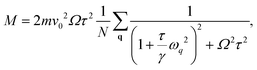
| | 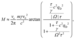 | (23) |
where
qD is the Debye frequency chosen as a cutoff for the integral over
q. For small
Ωτ the angular momentum grows linearly and can be approximated as:
| | 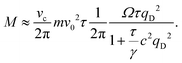 | (24) |
In contrast, for large values of Ωτ ≫ 1, the angular momentum decreases as  . This results in a non-monotonic dependence on Ω which is evident for different values of τ as shown in Fig. 4(c). This non-monotonicity can be understood by noting that for Ω = 0 (in the absence of chirality) the angular momentum vanishes due to symmetry. Similarly, we expect M to vanish again for Ω → ∞. This behavior arises because chirality induces a bending of the trajectories of an active particle, thereby reducing displacement fluctuations compared to the non-chiral case, eventually suppressing them entirely for sufficiently large chirality. This interpretation aligns with the findings from the study of a single chiral active particle in a harmonic potential.48 Let us note that, as demonstrated in Appendix D, the torque, T, exerted by the active chiral forces on the particles is balanced by the torque exerted by the friction, the latter being proportional to the angular momentum multiplied the friction coefficient, γ, yielding: |T| = γM.
We remark that even a collection of independent oscillators, all having the same frequency ω0 and subject to chiral active forces, would produce an angular momentum. In such a case, the value of M would be larger than the one of the solid described by eqn (22) because the particle interactions determine a spectrum containing frequencies ωq < ω0. The origin of the angular momentum of the system is induced by the chiral active force on each particle. In the absence of interactions among the particles, each particle would perform curved trajectories around its equilibrium position. The effect of the harmonic interactions is to couple the individual rotations so that the particles move in a more coherent fashion, i.e. the circular motion of each particle around its equilibrium position is concerted with the others. However, the infinite (N → ∞) ideal crystal considered in this paper does not show global rotations because the center of mass cannot move. However, global rotations emerge as a finite-size effect by considering a crystal consisting of chiral active particles subject to strong attractive interactions.80 Indeed, in this case, the center of mass of the crystal behaves itself as a chiral particle and thus is characterized by circular motion. Similar global rotations have been observed in a phase field model for chiral crystals94 or a system of interacting particles with active rotations.94
Steady-state entropy production rate of a chiral solid
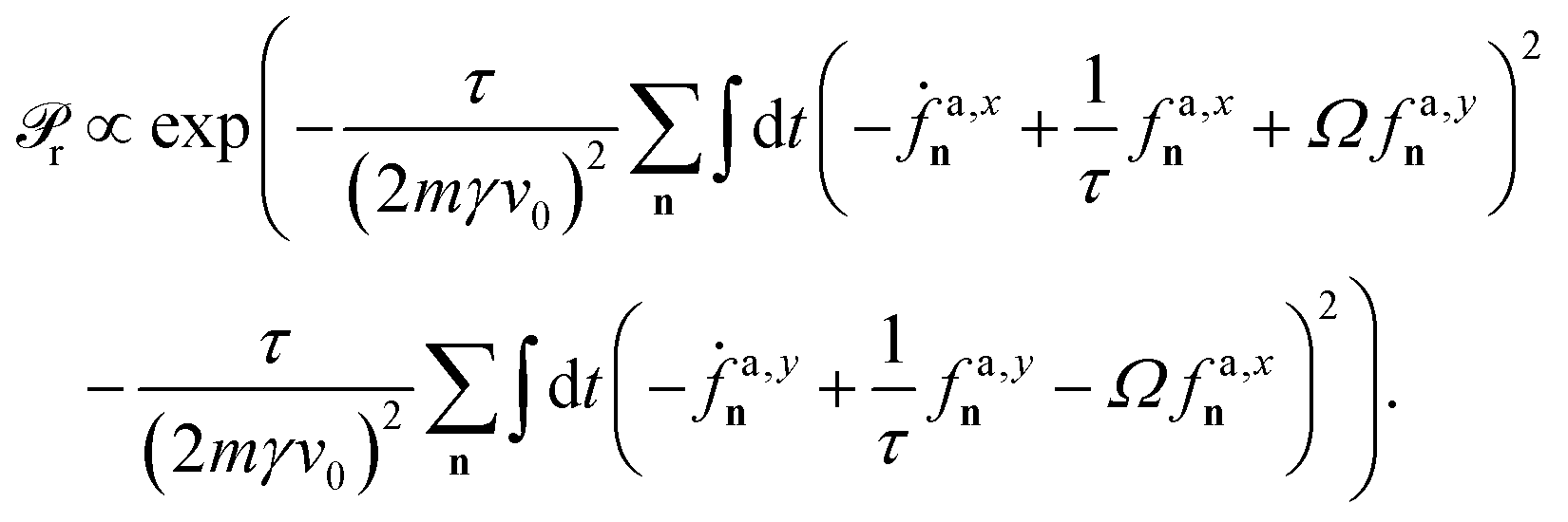
The entropy production serves as a measure of a system's irreversibility and its deviation from thermodynamic equilibrium.95–97 In systems far from equilibrium, time-reversal symmetry is broken, and detailed balance no longer holds. As a result, the probability of a stochastic trajectory (forward path) differs from the probability of its time-reversed counterpart (backward path). This asymmetry is quantified by the Kullback–Leibler divergence, expressed as the logarithm of the ratio between the probabilities, Pf, associated with forward paths, and Pr, associated with backward paths. This framework is used to define the entropy production rate, Ṡ98–100 as: 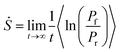 , where a non-zero value of Ṡ differentiates non-equilibrium steady states from equilibrium states. It is worth noting that this expression is often referred to as the entropy production rate of the medium. However, this term coincides with the entropy production rate in the steady state, which is the primary focus of our interest.
In the case of non-chiral active systems, each chiral active particle is intrinsically far from equilibrium100–107 and on average, each equally contributes to the entropy production rate. The total entropy production rate per particle of a chiral active crystal can be expressed as the sum of two contributions as:
The first term reads 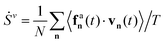 , and has the usual form of the entropy production rate of active particles, i.e. correspond to the work performed by the active force. The dependence on the chirality is implicitly contained in the equal-time correlations 〈fan(t)·vn(t)〉. Approximating this correlations, leads to the following result (see Appendix E)
| |  | (26) |
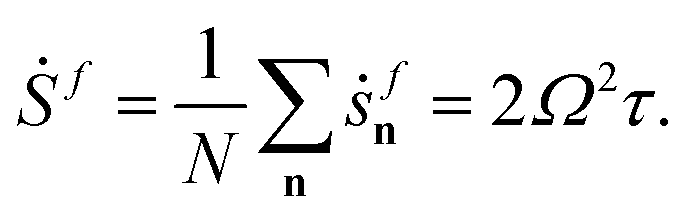
The entropy production rate contains an additional contribution arising from the active force dynamics, Ṡf, and given by the formula
| |  | (27) |
which is derived in Appendix E using a path integral approach to calculate forward and backward trajectories.
The term Sv (eqn (26)), representing the work performed by the active force, is intuitively non-zero because both the velocity and the active force tend to align, regardless of whether the particles are chiral or harmonically confined. Sv consists of two contributions: (i) a logarithmic term and (ii) an arctan term. (i) Has a functional form similar to that observed in non-chiral active particles, as discussed in ref. 92. Thus, this term can be naturally interpreted as a translational contribution arising from the tendency of active particles to persistently moving in a typical direction. Consistently with our interpretaiton, chirality reduces the magnitude of this term, which scales approximately as ∼1/Ω2 for large chirality values. By contrasts, the arctan contribution (ii) emerges from the angular drift present in the dynamics of the active force: it disappears for vanishing chirality (Ω = 0) and was not present in previous formulations of the entropy production rate for crystals consisting of non-chiral active particles. This is a rotational contribution to entropy production which is indeed proportional to the chirality-induced angular momentum (eqn (22) and (23)) or, in other words, the torque exerted by the chiral active force. Compared to non-chiral systems, the entropy production rate contains the additional term Ṡf which is entirely due to chirality and directly arises from the time evolution of the active force. This term represents the energetics cost needed to maintain a particle in rotational motion and generate a circular current. This contribution to entropy production is formally analog to the one obtained by applying path integral techniques to a Brownian particle subject to a quadratic central potential and rotating because of a magnetic field.
From this, we can immediately conclude that the interplay between these terms results in an entropy production rate that increases with chirality Ω. As Ω approaches zero, Ṡv tends to a finite limit, which corresponds to the entropy production rate of a solid composed of achiral AOUP particles. Conversely, Ṡv saturates for large values of Ω, while Ṡf vanishes at Ω = 0 and diverges quadratically as Ω approaches infinity.
Time-dependent correlations
In addition to decaying with particle separation, correlations also diminish over time. Understanding the time-dependent behavior of correlations is essential for unraveling the range and duration of collective effects in active matter systems.
As in the previous section, we will focus on the overdamped regime, where γ2/4 ≫ ωq2, to facilitate analytical progress and assess the impact of chirality. The temporal correlations, such as 〈ûαq(t)ûβ−q(0)〉 are obtained in the wave vector domain q. Temporal autocorrelations for the same particle coordinates are calculated by summing over q (or integrating over the Brillouin zone BZ):
| |  | (28) |
Time-dependent displacement and velocity correlations in the overdamped regime
After lengthy but straightforward calculations reported in Appendix C (see eqn (77) and (78)), we obtain the following formula for the displacement correlations with t ≥ 0:| |  | (29) |
where| |  | (30) |
By symmetry, we have 〈uyq(t)uy−q(0)〉 = 〈uxq(t)ux−q(0)〉. The first term in eqn (30) represents the contribution of thermal noise, while the second and third terms are due to the active force and have a non-equilibrium origin. Chirality reduces the amplitude of activity-induced fluctuations compared to the non-chiral case, leading to damped oscillatory behavior with frequency Ω, as evident from the presence of sin(Ωt) and cos(Ωt). We classify fluctuations based on their wavevector, q: (i) fluctuations with persistence times exceeding the viscous time associated with the mode of wavevector q (τ ≫ γ/ωq2). (ii) Long-wavelength fluctuations for which τ ≪ γ/ωq2. In the first case, the slowest relaxation modes are represented by terms proportional to  . For time separations t exceeding τ, the most relevant terms in the correlations vary exponentially as
  , with slower decay for smaller wavevectors q. After a short initial transient, the amplitude of these long-wavelength modes contributes significantly to real-space correlations.
Using eqn (79), we obtain the time correlation between diferent spatial components of displacement:
| |  | (31) |
where
| |  | (32) |
Exchanging the components (xy → yx) changes the sign of the correlation, i.e., 〈ûyq(t)ûx−q(0)〉 = −〈ûxq(t)ûy−q(0)〉, resulting in vanishing equal-time off-diagonal elements. In the short-time regime, the correlation varies linearly with t, contrasting with the diagonal correlation. Asymptotically (t ≫ τ), the leading term of the two-time correlation is proportional to Ωe−ωq2t/γ, with the prefactor being an odd function of Ω.
By using the method of Appendix C, we obtain the two-time diagonal elements of the velocity correlations, which can be expressed as follows:
| |  | (33) |
where
| |  | (34) |
Again, we can identify a thermal term proportional to T that decays with a characteristic time γ/ωq2 and a non-equilibrium term whose amplitude is given by the active temperature v02τγ. This second term is characterized by an exponential decay governed by two typical timescales: γ/ωq2 (as in the passive term) and the persistence time τ. As with displacement correlations, the chirality Ω induces temporal oscillations for a short duration.
By differentiating eqn (32), we derive the temporal velocity cross-correlations 〈![[v with combining circumflex]](https://www.rsc.org/images/entities/i_char_0076_0302.gif) xq(t)y−q(0)〉. Similar to the displacement in eqn (32), these correlations are antisymmetric with respect to the exchange of indices x and y, and vanish both at t = 0 and as t → ∞. Here, we simply present the expression in the long-time regime where ωq2τ/γ ≪ 1:
xq(t)y−q(0)〉. Similar to the displacement in eqn (32), these correlations are antisymmetric with respect to the exchange of indices x and y, and vanish both at t = 0 and as t → ∞. Here, we simply present the expression in the long-time regime where ωq2τ/γ ≪ 1:
| |  | (35) |
In the long-time regime, chirality contributes to these temporal correlations by decreasing their amplitude. This result is consistent with the reduction of persistence length for Ω > 0. Conversely, chirality induces circular trajectories, which manifest as short-time oscillations in the temporal correlations. These oscillations are neglected in the approximation of eqn (35).
Time-dependent density self-correlation function and mean-square-displacement
Although the harmonic lattice is a linear model, deriving an analytical expression for the self-density–density correlation is challenging due to its nonlinear dependence on the displacement correlation. We consider the average 〈ρn(x,t)ρn(x′,0)〉. The expression ρn(x,t) ≡ δ(2)(x − rn(t)) represents the probability density that the n-th particle is located at time t within a small volume centered around the point x.
Given the translational invariance of the system, we integrate over the entire volume and average over the distribution of particle positions. This leads us to define ![[capital G, script]](https://www.rsc.org/images/entities/char_e112.gif) inc(r,t) as follows: inc(r,t) = 〈δ(2)(rn(0) + r − rn(t))〉. Using the displacement variables and the Fourier representation of the Dirac delta function we have:
inc(r,t) as follows: inc(r,t) = 〈δ(2)(rn(0) + r − rn(t))〉. Using the displacement variables and the Fourier representation of the Dirac delta function we have:
| |  | (36) |
where MSD(
t) = 〈(
un(
t) −
un(0))
2〉. In the Gaussian expression above, the dependence on the chiral parameter
Ω is embedded within the mean square displacement, MSD(
t), which can be computed by using the Green–Kubo relation,
i.e. by double integrating over time the autocorrelation of the velocity
(33) and then performing the integration over the wave vector
q. This leads to the following formula:
| |  | (37) |
where
| |  | (38) |
| |  | (39) |
This observable provides insight into the particle's ability to explore the space and is illustrated in Fig. 5(a) through the direct integration of formula (38) for various values of chirality, Ω, using an upper cutoff qD. Notably, the MSD(t) displays a quadratic growth with respect to t in the short-time regime t < τ:
| |  | (40) |
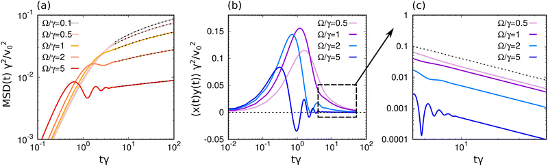 |
| | Fig. 5 Time-dependent properties. (a) Mean-square-displacement MSD(t) = 〈(un(t) − un(0))2〉 as a function of time t for different values of the chirality Ω/γ normalized by the inertial time. Colored lines are obtained by integrating eqn (38) over q while black dashed lines are realized by fitting a logarithm function a![[thin space (1/6-em)]](https://www.rsc.org/images/entities/char_2009.gif) log(tb) where a and b are fitting parameters. These fits confirm the approximation (41). (b) and (c) Temporal cross correlation 〈uxn(t)uyn(0)〉 as a function of time t for different values of Ω/γ. Colored lines are obtained by integrating eqn (32) over q. (c) Is a zoom on the square area in panel (b), where the 1/t scaling is shown as a black dashed line. In all the panels, the curves are obtained with mv02/T = 102 and K/(γ2m) = 103 and τγ = 1. log(tb) where a and b are fitting parameters. These fits confirm the approximation (41). (b) and (c) Temporal cross correlation 〈uxn(t)uyn(0)〉 as a function of time t for different values of Ω/γ. Colored lines are obtained by integrating eqn (32) over q. (c) Is a zoom on the square area in panel (b), where the 1/t scaling is shown as a black dashed line. In all the panels, the curves are obtained with mv02/T = 102 and K/(γ2m) = 103 and τγ = 1. | |
The variance 〈![[v with combining circumflex]](https://www.rsc.org/images/entities/b_char_0076_0302.gif) q(0)−q(0)〉 is given by eqn (33) at t = 0 and depends on the swim velocity and chirality. This t2 behavior is typical of active matter systems and arises from the self-propulsion force, which induces ballistic behavior over short time scales. For sufficiently large chirality compared to the persistence time, such that Ωτ > 1, the mean squared displacement, MSD(t), displays oscillations which become more pronounced as Ω increases (Fig. 5(a)). These oscillations emerge for intermediate times and are suppressed in the long-time regime, where the dominant contribution to the integral comes from the small wavevector region. Consequently, the long-time behavior can be approximated as follows:
q(0)−q(0)〉 is given by eqn (33) at t = 0 and depends on the swim velocity and chirality. This t2 behavior is typical of active matter systems and arises from the self-propulsion force, which induces ballistic behavior over short time scales. For sufficiently large chirality compared to the persistence time, such that Ωτ > 1, the mean squared displacement, MSD(t), displays oscillations which become more pronounced as Ω increases (Fig. 5(a)). These oscillations emerge for intermediate times and are suppressed in the long-time regime, where the dominant contribution to the integral comes from the small wavevector region. Consequently, the long-time behavior can be approximated as follows:
| |  | (41) |
The MSD(t) exhibits a logarithmic divergence with respect to t, similar to the passive case. Indeed, expression (41) contains a passive contribution proportional to T and an active contribution proportional to the active temperature v02τγ. The latter is reduced by chirality as evident in Fig. 5(a). Additionally, chirality induces a temporal profile in the cross-correlations, 〈uxn(t)uyn(0)〉, obtained by numerically integrating eqn (32) over q using the continuum approximation (28). Fig. 5(b) displays this observable as a function of time for various values of Ω. Rather than presenting the lengthy expressions, we will concentrate on the short-time and long-time regimes. The short-time regime exhibits linear growth, which can be approximated by:
| |  | (42) |
Conversely, in the long-time regime, employing the same methodology as in deriving eqn (41), yields the expression:
| |  | (43) |
Thus, for large t, temporal cross-correlations have a long-range ∼1/t decrease. In agreement with the previous observations in the frequency and wave vector representation, the coefficients of the cross-correlations are non-monotonic functions of the chirality Ω.
Summary and conclusions
In this paper, we studied a two-dimensional harmonic solid composed of chiral active particles, which are modeled by incorporating an angular drift into the active force term. We analyzed the displacement and velocity correlation functions in both the time and frequency domains. A harmonic chiral active crystal adheres to the Mermin–Wagner theorem, exhibiting a diverging displacement–displacement correlation in two dimensions. Furthermore, as in the non-chiral case, these chiral crystals display spatial velocity correlations. While chirality does not significantly alter the functional form of these correlations, it reduces their correlation length. This result is consistent with the continuum theoretical approach and the numerical results obtained by Shee et al.77 In ref. 77, a more realistic description of the chiral solid is adopted by considering high-density chiral active particles interacting with linear repulsion. Our theory, which does not involve any fitting parameter, can be compared with the non-linear model by setting a high effective elastic constant (extremely high density) so that the displacements are not too large. We leave this comparison for a future investigation.
The distinctive properties of chiral crystals are highlighted by a non-vanishing angular momentum, defined as the vector product of the displacement and velocity of the particles. The angular momentum stems from the torque exerted by the active force, which has a preferential direction due to chirality. The angular momentum, which is zero for a crystal consisting of non-chiral active particles, shows a non-monotonic dependence on chirality and possesses a spatial structure. Chirality also influences the dynamical properties of the crystal by altering the spectrum of particle displacements, introducing a non-dispersive peak at the chiral frequency. This peak is not altered by the presence of inertia and coexists with the phononic peak (underdamped regime) or the peak at vanishing frequency (overdamped regime). Moreover, the unique effects of chirality manifest in non-zero cross-correlations between different Cartesian components of displacement–displacement and velocity–velocity dynamical correlations in the frequency domain. The presence of this peak leads to temporal oscillations in the autocorrelations of particle displacement and mean-square displacement, which we have analytically predicted. Finally, chirality contributes an additional entropy production term, specifically associated with angular momentum.
Our findings provide analytical insights into recent phenomena displayed by chiral active particles and may lead to novel applications. Our results suggest that chirality represents a strategy to design crystals with a non-dispersive peak at a specific frequency. This frequency is uniquely selected by chirality and can be responsible for resonant effects due to the superposition with phononic peaks. The theory developed in this paper for an ideal chiral active crystal may pave the way for the investigation of isolated topological defects or weak mass defects in solid structures. This problem can be tackled analytically by resorting to perturbative techniques around the ideal solution, for instance following the method adopted in ref. 108 for a non-chiral active crystal with isolated defects. Additionally, our study is consistent and, somehow, provides a theoretical justification for the emergence of Magnus effects observed in the dynamics of a probe particle driven by a constant force in a chiral active bath.42,43,109–112 These Magnus effects have been observed numerically for different densities of the environment exploring both liquid-like or solid-like configurations. This phenomenon can happen if the environment is characterized by cross-correlations (for instance, coupling the x and y components of the displacement field), as we have predicted for an ideal chiral active crystal. We expect that chiral active liquids display similar correlations which can be numerically explored.
Beyond the numerical investigation of a densely packed assembly of chiral soft spheres,17,113 our predictions can be tested in experimental active matter systems exhibiting chirality. Promising candidates include systems of densely packed chiral active colloids114 or colloids subjected to a magnetic field, starfish embryos115 as well as active granular particles.91,116–118 In the latter macroscopic setups, particles can be connected using rigid rods39 or springs,119 while chirality can be introduced by modifying the particle shape.36–38 In all these cases, our findings can be tested through standard data acquisition techniques by using standard imaging systems and high-speed cameras which allow for the calculation of the displacement field and, thus, displacement–displacement dynamical correlations.
We remark that the model employed in this paper fundamentally differs from particle-based models characterized by transverse interactions,120 recently employed to describe odd elastic solids. In the latter case, rotations are induced by particle interactions and, thus, represent a two-body effect, while the circular motion observed in a chiral active Brownian particle is a single-body property. Consequently, while our model is always linearly stable, the model of Choi et al. presents a rich phase diagram comprising no-waves, damped or persistent waves, and a melted phase.120 However, our exactly solvable model may bridge the gap between macroscopic theories of chiral crystals with odd elastic properties.31,120 These macroscopic elastodynamic theories rely on an antisymmetric elastic matrix. By employing coarse-graining techniques, one can derive the effective elastic matrix for our model, providing insights into the relation between chirality and odd elasticity.
Data availability
The data supporting this article have been included as part of the Appendices. Indeed, these Appendices contains the theoretical predictions that are plotted in the main text.
Conflicts of interest
There are no conflicts to declare.
Appendices
Definition of time and space Fourier transforms
Fourier transforms are performed in the time and space domains. Even if the explicit dependence on frequency ω (time t) or wave vector q (particle index n) is always explicit, we adopt the following notation: (i) a vertical bar over the variable denotes time Fourier transform in the domain (ω, n). (ii) The hat is used for the spatial Fourier transform in the domain (t, q). (iii) The tilde is employed for the time and space Fourier transforms in the domain (ω, q). Specifically, we define the time Fourier transform of the particle displacement, which is denoted by the tilde symbol and an explicit dependence on the frequency ω, as| |  | (44) |
while the inverse time Fourier transform reads| |  | (45) |
Similar definitions hold for the other variables, such as velocity, active force and noise variables. Specifically, delta-correlated white noises, such that 〈ξn(t)ξm(t′)〉 = δ(t − t′)δnm, satisfy the following relation in Fourier space
| |  | (46) |
and

. In a similar way, we can define the discrete spatial Fourier transform of the displacemente vector as
| |  | (47) |
where
Rn is a vector identifying the position of each lattice site and
q = (
qx,
qy) is a discrete wave vector and
N is the total number of particles. The inverse discrete spatial Fourier transform is defined as
| |  | (48) |
The combination of the time and space Fourier transforms leads to the definition (5).
Derivation of the dynamical correlations
In this Appendix, we derive the dynamical correlation of the particle displacement in the frequency ω and wave vector q domains, i.e.eqn (8) and (9). As a first step to finding analytical solutions, we consider the Fourier transforms in time and space of the dynamics (2) for the active force and the dynamics (4) for the particle displacement. Specifically, the Fourier transform of the active force dynamics expressed in Cartesian components reads:| |  | (49a) |
| |  | (49b) |
where we have used superscript to denote the x or y Cartesian component. By contrast, the Fourier transform of the displacement dynamics reads| |  | (50) |
which corresponds to eqn (6) upon defining 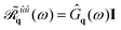 via the propagator Ĝq(ω), introduced below eqn (6). We remark that the Fourier transforms of the white noises satisfy the following properties:
| | 〈![[small chi, Greek, tilde]](https://www.rsc.org/images/entities/i_char_e11b.gif) αq(ω)β−q(ω′)〉 = 2πδαβδ(ω + ω′) αq(ω)β−q(ω′)〉 = 2πδαβδ(ω + ω′) | (51) |
| | 〈![[small xi, Greek, tilde]](https://www.rsc.org/images/entities/i_char_e119.gif) αq(ω)β−q(ω′)〉 = 2πδαβδ(ω + ω′), αq(ω)β−q(ω′)〉 = 2πδαβδ(ω + ω′), | (52) |
where α,β = x,y denote Cartesian components.
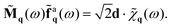
Active force self correlation function in ω representation
The linearity of the dynamics for the active force, eqn (49a) and (49b), allows us to solve the dynamics. Let us introduce for convenience the dynamical matrix q(ω) as| | 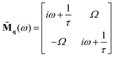 | (53) |
and the diffusive matrix D = ddT where T means transpose matrix and  .
.
The active force dynamics in the Fourier space (49a) and (49b) can be expressed in a matrix form as
| |  | (54) |
Dynamical correlations of the active force are defined as the elements of the matrix 〈![[f with combining tilde]](https://www.rsc.org/images/entities/b_char_0066_0303.gif) aq × (aq)T〉, where T means transpose and 〈·〉 is the average over the noise realizations. These dynamical correlations can be obtained by multiplying the dynamics (54) by q−1(ω) on the left and by (aq)T on the right and then taking the average over the noise realizations. Indeed, in this way, we get
aq × (aq)T〉, where T means transpose and 〈·〉 is the average over the noise realizations. These dynamical correlations can be obtained by multiplying the dynamics (54) by q−1(ω) on the left and by (aq)T on the right and then taking the average over the noise realizations. Indeed, in this way, we get
| | 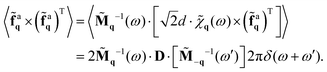 | (55) |
By following this strategy, we can obtain the elements of the dynamical correlations which are reported below
| |  | (56a) |
| |  | (56b) |
where the remaining elements satisfy the following relations
| | 〈![[f with combining tilde]](https://www.rsc.org/images/entities/i_char_0066_0303.gif) a,xq(ω)a,x−q(−ω)〉 = 〈a,yq(ω)a,y−q(−ω)〉 a,xq(ω)a,x−q(−ω)〉 = 〈a,yq(ω)a,y−q(−ω)〉 | (57) |
| | | 〈a,xq(ω)a,y−q(−ω)〉 = −〈a,yq(ω)a,x−q(−ω)〉. | (58) |
Displacement–displacement correlation function in ω representation
In a similar way, we can solve the linear dynamics for the particle displacement, i.e.eqn (6) (or equivalently eqn (50)). By multiplying the dynamics (50) by ũx−q(−ω) or ũy−q(−ω) and taking the average over the noise realization, we can express the dynamical correlations of the particle displacement| |  | (59) |
| |  | (60) |
Finally, we write the (q,ω) representation of the displacement–displacement correlation function
| |  | (61) |
| |  | (62) |
Again, the remaining matrix elements satisfy the relations
| | | 〈ũxq(ω)ũx−q(−ω)〉 = 〈ũyq(ω)ũy−q(−ω)〉 | (63) |
| | | 〈ũxq(ω)ũy−q(−ω)〉 = −〈ũyq(ω)ũx−q(−ω)〉. | (64) |
eqn (61) and (62) correspond to
eqn (8) and (9), respectively.
Spectral representation of the active torque
We first demonstrate that the spectral density of the angular momentum is proportional to the spectral density of the torque generated by the active force. By multiplying the displacement dynamics (50) by ũ−q(−ω) via the cross product and averaging over the noise realizations, we have:| |  | (65) |
where we have used that the correlation between noise and displacement vanish. By summing to this equation its complex conjugate, we have| | 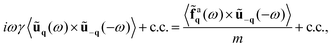 | (66) |
and, finally, by substituting −iωũ−q(−ω) → ṽ−q(−ω), we obtain the desired proportionality between angular momentum and torque:| | | γ〈ũq(ω) × ṽ−q(−ω) + c.c.〉 = 〈ũq(ω) × a−q(−ω) + c.c.〉. | (67) |
The torque generated by the active force can be calculated by multiplying the dynamics (50) by a−q(ω′) and taking the average over the noise realizations. Within this protocol, we obtain
| |  | (68) |
where we have used that the correlations between translational noise and active forces vanish. The torque and, thus, the angular momentum can be obtained by using the expressions for the dynamical correlations of the active force
(56). In this way, we get
| |  | (69) |
which leads to the spectral density of the angular momentum
(10) by diving
eqn (69) by
γ.
Time correlations
In the present Appendix, we derive the time correlations in the overdamped limit by solving in the time domain the dynamical equations of the model, whose dynamics reads:| |  | (70) |
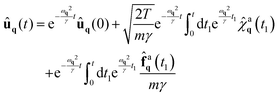
We first consider the following integral representation of the solutions of eqn (2), obtained for zero initial value of the active force:
| |  | (71) |
where

and
λ* is its complex conjugate. The solution of the overdamped
eqn (70) is given by
| |  | (72) |
where the first and second term represent the homogeneous part of the solution and the contribution due to the thermal noise and the last term the effect of the activity.
Displacement–displacement time correlation
Putting together eqn (71) and (72) we obtain the following expression for the part of the displacement due to the chiral active force:
that can be rewritten as| |  | (73) |
where we used the definition| |  | (74) |
After an integration by parts, we may rewrite it as a simple integral
| |  | (75) |
For subsequent applications, we define the function Hα(t;λ):
| |  | (76) |
With the help of formula (73) we can write the correlators as
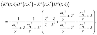
| |  | (77) |
where the angular brackets represent the double average over the thermal noise and the realisations of active noise. using the following properties of the averages 〈
Kx(
t;
λ)
Kx(
t′;
λ*)〉 = 〈
Ky(
t;
λ)
Ky(
t′;
λ*)〉 and 〈
Kx(
t;
λ)
Kx(
t′;
λ)〉 = 〈
Ky(
t;
λ)
Ky(
t′;
λ)〉, we find
| |  | (78) |
Performing the calculations after simple algebra we find the result of eqn (30). Similarly, we obtain the off diagonal correlation function:
| |  | (79) |
Explicitly:
| |  | (80) |
leading to formula
(32). To obtain the cross correlation, 〈
ûyq(
t)
ûx−q(
t′)〉, we use the property
| | | 〈ûyq(t)ûx−q(t′)〉 = −〈ûxq(t)ûy−q(t′)〉 | (81) |
from which it follows that the equal-time cross correlations vanish:
| | | 〈ûyq(t)ûx−q(t)〉 = −〈ûxq(t)ûy−q(t)〉 = 0. | (82) |
Velocity–velocity time-correlation
The velocity correlations can be computed by differentiating the displacement correlation function with respect to its two arguments, t and t′:| |  | (83) |
and a similar method is employed to determine the off diagonal velocity correlation. The relative results are given in the main text eqn (33) and (35). Evaluating eqn (83) at t = t′, one obtains:| | 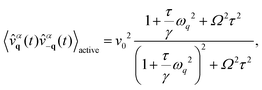 | (84) |
which corresponds to eqn (16).
Torque and angular momentum
Let us consider T, the average total torque exerted by the active forces on the particles. Its expression is:| |  | (85) |
On the other hand the average total angular momentum is
| |  | (86) |
To evaluate the average angular momentum (86), we consider the time derivative of the displacement correlation:
| |  | (87) |
If one considers t > t′ but both t and t′ are ≫τ and ≫1/γ, one obtains the result:
| |  | (88) |
After some algebra, we obtain:
| |  | (89) |
In order to evaluate the average torque (85) exerted on the q mode we consider the following cross correlation:
| |  | (90) |
Performing the integrals and averaging over realizations we find
| |  | (91) |
A brief calculation yields the following result:
| |  | (92) |
By comparison with eqn (89) one obtains that the torque exerted by the frictional forces represented by formula (92) is equal to the angular momentum multiplied by γ. In other words, the torque exerted by the active forces is balanced by the frictional torque exerted by the medium.
Derivation of the entropy production formula
To use the definition and calculate the total entropy production rate Ṡ, we use a path-integral approach to estimate the probability of forward and backward trajectories. As usual, the particles' trajectories are fully determined by the noise path. For a chiral active systems, the noise probability has a Gaussian form for each noise governing the dynamics at each time, ξ(t) and χ(t). By using curly bracket to denote a noise trajectory from an initial time t0 to a final time tf for every particle of the system, i.e. ({ξ},{χ}), the path probability of the noise reads| | 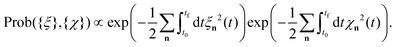 | (93) |
By expressing each noise as a function of the dynamical variables xn, vn, and fanvia by using the equation of motion
| |  | (94a) |
| | 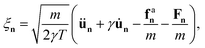 | (94b) |
one can easily switch from the probability of the noise Prob({
ξ} to the probability of the trajectory
![[scr P, script letter P]](https://www.rsc.org/images/entities/char_e52f.gif) f
f(({
v},{
v},{
fa}) by applying a change of variables. Since the Jacobian of this transformation does not affect the entropy production,
100 we can explicitly write
| | 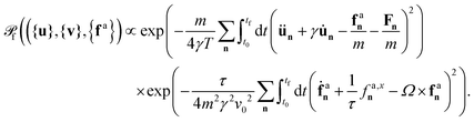 | (95) |
The probability of the backward trajectory f can be obtained by applying the following transformations
to the particle dynamics, and consequently to the relations in (94), which are involved in the path probability. The assumption of even position and odd velocity under time-reversal transformation appears natural. In contrast, assuming an even active force is less straightforward and has recently sparked debate within the active matter community.95,100,121,122 When calculating the log ratio of the path probabilities, each noise source contributes an additional term. Therefore, we will separately calculate the contributions to the entropy production rate arising from the thermal noise ξn, governing the velocity dynamics, and the noise χn, controlling the active force dynamics. In other words, the total entropy production rate can be decomposed into the sum of two terms
where the subscripts highlight the origin of the entropy production rate:
v for velocity dynamics and
f for active force dynamics.
Contribution of the velocity dynamics to entropy production
The Contribution of the velocity dynamics to the entropy production rate can be calculated by restricting to the first exponential in the expression (95). We remark that this calculation is formally equivalent to the one for non-chiral particles and, indeed, it leads to the same result. Indeed, by considering the log ratio of the forward and backward trajectories in this exponential contribution, we obtain| | 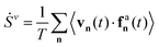 | (98) |
where b.t. denotes boundary terms that vanish in the infinite time limit, i.e. the potential and kinetic energy. This term coincides with the first term in eqn (25).
Calculating Ṡv requires to estimate the equal time correlation appearing in eqn (98). Employing eqn (71), (73), and (76), the product the velocity of the particles and the active force can be represented as:
| |  | (99) |
When t → ∞ and t′ → ∞ but (t − t′) ≥ 0 remains finite so that for t = t′ we obtain:
| |  | (100) |
and use the property of the averages: 〈
Kx(
t;
λ)
Hx(
t′;
λ*)〉 = 〈
Ky(
t;
λ)
Hy(
t′;
λ*)〉. Finally, we find
| | 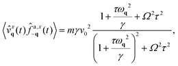 | (101) |
which reduces to
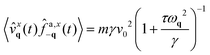
in the achiral case,
Ω = 0. The entropy rate production of the mode
q is given by
| | 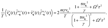 | (102) |
From here, we can calculate the velocity-active force correlation in real space, and thus entropy production, by integrating over the wave vector q, as done in Section 4. This leads to the following expression for the velocity contribution to the entropy production rate of the system Ṡv:
| | 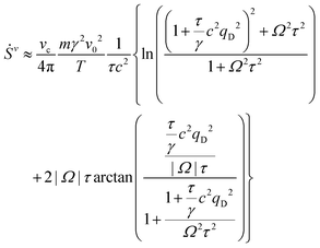 | (103) |
which corresponds to
eqn (26).
Contribution of the active force dynamics to entropy production
In this section, we calculate the contribution to entropy production of the active force dynamics, i.e. Ṡf. To increase the clarity of this calculation, here we report the path probabilities related to the active force dynamics in Cartesian components| |  | (104) |
In agreement with previous work, we assume that the active force is even under time-reversal transformation, such that fan → fan when t → −t. The probability of the reversed path r associated to the active force dynamics reads:
| | 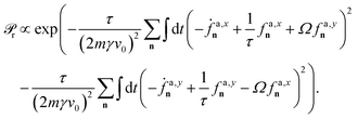 | (105) |
By taking the ratio ln(f/r), applying the average and dividing by the time interval, we obtain the entropy production definition. Since noises of different particles are independent we have:
| |  | (106) |
where
ṡfn is the entropy production of the medium per particle, that is
| | 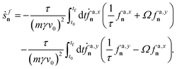 | (107) |
In the previous expression, only cross terms xy survive providing a contribution to entropy production rate per particle which reads
| |  | (108) |
where
t =
tf −
t0. Finally, by using
eqn (3b) and (3c)| |  | (109) |
we obtain the final result which has the following form in the infinite time limit,
i.e. for (
tf −
t0) → ∞:
| |  | (110) |
This expression gives the contribution of the active bath to the entropy production rate reported in eqn (27).
Acknowledgements
LC and UMBM acknowledge Andrea Puglisi for useful discussions.
Notes and references
- A. K. Pal and B. Bahadur, Int. J. Life Sci., 2020, 9, 72–84 CrossRef.
-
A. A. Sinjushin and B. Bahadur, Asymmetry in Plants, CRC Press, 2019, pp. 105–120 Search PubMed.
- M. Marchetti, J. Joanny, S. Ramaswamy, T. Liverpool, J. Prost, M. Rao and R. A. Simha, Rev. Mod. Phys., 2013, 85, 1143–1189 CrossRef.
- J. Elgeti, R. G. Winkler and G. Gompper, Rep. Prog. Phys., 2015, 78, 056601 CrossRef.
- C. Bechinger, R. Di Leonardo, H. Löwen, C. Reichhardt, G. Volpe and G. Volpe, Rev. Mod. Phys., 2016, 88, 045006 CrossRef.
- H. Löwen, Eur. Phys. J.:Spec. Top., 2016, 225, 2319–2331 Search PubMed.
- B. Liebchen and D. Levis, EPL, 2022, 139, 67001 CrossRef CAS.
- T. Vicsek and A. Zafeiris, Phys. Rep., 2012, 517, 71–140 CrossRef.
- A. Cavagna and I. Giardina, Annu. Rev. Condens. Matter Phys., 2014, 5, 183–207 CrossRef CAS.
- M. E. Cates and J. Tailleur, Annu. Rev. Condens. Matter Phys., 2015, 6, 219–244 CrossRef.
- S. Mandal, B. Liebchen and H. Löwen, Phys. Rev. Lett., 2019, 123, 228001 CrossRef PubMed.
- M. N. Van Der Linden, L. C. Alexander, D. G. A. L. Aarts and O. Dauchot, Phys. Rev. Lett., 2019, 123, 098001 CrossRef PubMed.
- C. B. Caporusso, P. Digregorio, D. Levis, L. F. Cugliandolo and G. Gonnella, Phys. Rev. Lett., 2020, 125, 178004 CrossRef PubMed.
- L. Caprini, R. K. Gupta and H. Löwen, Phys. Chem. Chem. Phys., 2022, 24, 24910–24916 RSC.
- L. Caprini, U. M. B. Marconi and A. Puglisi, Phys. Rev. Lett., 2020, 124, 078001 CrossRef PubMed.
- S. Henkes, K. Kostanjevec, J. M. Collinson, R. Sknepnek and E. Bertin, Nat. Commun., 2020, 11, 1405 CrossRef PubMed.
- L. Caprini and U. M. B. Marconi, Soft Matter, 2021, 17, 4109–4121 RSC.
- G. Szamel and E. Flenner, EPL, 2021, 133, 60002 CrossRef.
- Y.-E. Keta, J. U. Klamser, R. L. Jack and L. Berthier, Phys. Rev. Lett., 2024, 132, 218301 CrossRef PubMed.
- L. Abbaspour, R. Mandal, P. Sollich and S. Klumpp, Commun. Phys., 2024, 7, 289 CrossRef.
- W. Uspal, M. N. Popescu, S. Dietrich and M. Tasinkevych, Soft Matter, 2015, 11, 434–438 RSC.
- R. Wittmann and J. M. Brader, EPL, 2016, 114, 68004 CrossRef.
- L. Caprini and U. M. B. Marconi, Soft Matter, 2018, 14, 9044–9054 RSC.
- S. Das, G. Gompper and R. G. Winkler, New J. Phys., 2018, 20, 015001 CrossRef.
- C. Hargus, J. M. Epstein and K. K. Mandadapu, Phys. Rev. Lett., 2021, 127, 178001 CrossRef CAS.
- E. Kalz, H. D. Vuijk, I. Abdoli, J.-U. Sommer, H. Löwen and A. Sharma, Phys. Rev. Lett., 2022, 129, 090601 CrossRef CAS PubMed.
- E. Kalz, H. D. Vuijk, J.-U. Sommer, R. Metzler and A. Sharma, Phys. Rev. Lett., 2024, 132, 057102 CrossRef CAS.
- D. Banerjee, A. Souslov, A. G. Abanov and V. Vitelli, Nat. Commun., 2017, 8, 1–12 CrossRef.
- M. Han, M. Fruchart, C. Scheibner, S. Vaikuntanathan, J. J. De Pablo and V. Vitelli, Nat. Phys., 2021, 17, 1260–1269 Search PubMed.
- X. Lou, Q. Yang, Y. Ding, P. Liu, K. Chen, X. Zhou, F. Ye, R. Podgornik and M. Yang, Proc. Natl. Acad. Sci. U. S. A., 2022, 119, e2201279119 CrossRef CAS.
- M. Fruchart, C. Scheibner and V. Vitelli, Annu. Rev. Condens. Matter Phys., 2023, 14, 471–510 CrossRef.
- F. Kümmel, B. ten Hagen, R. Wittkowski, I. Buttinoni, R. Eichhorn, G. Volpe, H. Löwen and C. Bechinger, Phys. Rev. Lett., 2013, 110, 198302 CrossRef.
- P. A. Monderkamp, R. S. Windisch, R. Wittmann and H. Löwen, J. Chem. Phys., 2023, 158, 164505 CrossRef CAS.
- X. Cao, D. Das, N. Windbacher, F. Ginot, M. Krüger and C. Bechinger, Nat. Phys., 2023, 19, 1904–1909 Search PubMed.
- L. N. Carenza, G. Gonnella, D. Marenduzzo and G. Negro, Proc. Natl. Acad. Sci. U. S. A., 2019, 116, 22065–22070 CrossRef CAS.
- C. Scholz, M. Engel and T. Pöschel, Nat. Commun., 2018, 9, 931 Search PubMed.
- F. Vega Reyes, M. A. López-Castaño and Á. Rodrguez-Rivas, Commun. Phys., 2022, 5, 256 Search PubMed.
- C. Scholz, A. Ldov, T. Pöschel, M. Engel and H. Löwen, Sci. Adv., 2021, 7, eabf8998 CrossRef.
-
L. Caprini, I. Abdoli, U. M. B. Marconi and H. Löwen, arXiv, 2024, preprint, arXiv:2410.02567, DOI:10.48550/arXiv.2410.02567.
- S. Van Teeffelen and H. Löwen, Phys. Rev. E:Stat., Nonlinear, Soft Matter Phys., 2008, 78, 020101 CrossRef.
- F. J. Sevilla, Phys. Rev. E, 2016, 94, 062120 CrossRef PubMed.
- C. Reichhardt and C. O. Reichhardt, Phys. Rev. E, 2019, 100, 012604 CrossRef PubMed.
- O. Chepizhko and T. Franosch, New J. Phys., 2020, 22, 073022 CrossRef.
- D. M. Van Roon, G. Volpe, M. M. T. da Gama and N. A. Araújo, Soft Matter, 2022, 18, 6899–6906 RSC.
- K. S. Olsen, Phys. Rev. E, 2021, 103, 052608 CrossRef PubMed.
- H. Shi, X. Zhao, W. Guo, J. Fang and L. Du, Nonlinear Dyn., 2024, 112, 21085–21096 CrossRef.
- P. L. Muzzeddu, H. D. Vuijk, H. Löwen, J.-U. Sommer and A. Sharma, J. Chem. Phys., 2022, 157, 134902 CrossRef.
- L. Caprini, H. Löwen and U. Marini Bettolo Marconi, Soft Matter, 2023, 19, 6234–6246 RSC.
- L. Caprini and U. M. B. Marconi, Soft Matter, 2019, 15, 2627–2637 RSC.
- Z. Fazli and A. Naji, Phys. Rev. E, 2021, 103, 022601 CrossRef.
- J. Mecke, Y. Gao, G. Gompper and M. Ripoll, Commun. Phys., 2024, 7, 332 CrossRef.
-
B. Valecha, P. L. Muzzeddu, J.-U. Sommer and A. Sharma, arXiv, 2024, preprint, arXiv:2409.18703, DOI:10.48550/arXiv.2409.18703.
- B. Liebchen and D. Levis, Phys. Rev. Lett., 2017, 119, 058002 CrossRef PubMed.
- D. Levis and B. Liebchen, J. Phys.: Condens. Matter, 2018, 30, 084001 CrossRef PubMed.
- B.-Q. Ai, Z.-G. Shao and W.-R. Zhong, Soft Matter, 2018, 14, 4388–4395 RSC.
- N. Kruk, J. A. Carrillo and H. Koeppl, Phys. Rev. E, 2020, 102, 022604 CrossRef PubMed.
- G.-J. Liao and S. H. Klapp, Soft Matter, 2021, 17, 6833–6847 RSC.
- A. Negi, K. Beppu and Y. T. Maeda, Phys. Rev. Res., 2023, 5, 023196 CrossRef CAS.
- B.-Q. Zhang and Z.-G. Shao, Phys. A, 2022, 598, 127373 CrossRef.
- K. L. Kreienkamp and S. H. Klapp, New J. Phys., 2022, 24, 123009 CrossRef.
- T. Hiraiwa, R. Akiyama, D. Inoue, A. M. R. Kabir and A. Kakugo, Phys. Chem. Chem. Phys., 2022, 24, 28782–28787 RSC.
- T. Lei, C. Zhao, R. Yan and N. Zhao, Soft Matter, 2023, 19, 1312–1329 RSC.
- A. Negi, K. Beppu and Y. T. Maeda, Phys. Rev. Res., 2023, 5, 023196 CrossRef CAS.
- S. Ceron, K. O’Keeffe and K. Petersen, Nat. Commun., 2023, 14, 940 CrossRef CAS PubMed.
- P. Arora, A. Sood and R. Ganapathy, Sci. Adv., 2021, 7, eabd0331 CrossRef CAS PubMed.
- B. Liebchen, M. E. Cates and D. Marenduzzo, Soft Matter, 2016, 12, 7259–7264 RSC.
- G.-J. Liao and S. H. Klapp, Soft Matter, 2018, 14, 7873–7882 RSC.
- Z. Ma and R. Ni, J. Chem. Phys., 2022, 156, 021102 CrossRef.
- V. Semwal, J. Joshi, S. Dikshit and S. Mishra, Phys. A, 2024, 634, 129435 CrossRef.
- E. Sesé-Sansa, D. Levis and I. Pagonabarraga, J. Chem. Phys., 2022, 157, 224905 Search PubMed.
- J. Bickmann, S. Bröker, J. Jeggle and R. Wittkowski, J. Chem. Phys., 2022, 156, 194904 Search PubMed.
- Q.-L. Lei, M. P. Ciamarra and R. Ni, Sci. Adv., 2019, 5, eaau7423 CrossRef PubMed.
- M. Huang, W. Hu, S. Yang, Q.-X. Liu and H. Zhang, Proc. Natl. Acad. Sci. U. S. A., 2021, 118, e2100493118 CrossRef PubMed.
- B. Zhang and A. Snezhko, Phys. Rev. Lett., 2022, 128, 218002 CrossRef PubMed.
- Y. Kuroda and K. Miyazaki, J. Stat. Mech.:Theory Exp., 2023, 2023, 103203 CrossRef.
- Y. Kuroda, T. Kawasaki and K. Miyazaki, Phys. Rev. Res., 2025, 7, L012048 CrossRef.
- A. Shee, S. Henkes and C. Huepe, Soft Matter, 2024, 20, 7865–7879 RSC.
- V. E. Debets, H. Löwen and L. M. Janssen, Phys. Rev. Lett., 2023, 130, 058201 CrossRef PubMed.
- B. Zhang, A. Sokolov and A. Snezhko, Nat. Commun., 2020, 11, 4401 CrossRef PubMed.
- L. Caprini, B. Liebchen and H. Löwen, Commun. Phys., 2024, 7, 153 CrossRef.
- E. Lauga, W. R. DiLuzio, G. M. Whitesides and H. A. Stone, Biophys. J., 2006, 90, 400–412 CrossRef PubMed.
- A. P. Petroff, X.-L. Wu and A. Libchaber, Phys. Rev. Lett., 2015, 114, 158102 CrossRef PubMed.
- E. Perez Ipiña, S. Otte, R. Pontier-Bres, D. Czerucka and F. Peruani, Nat. Phys., 2019, 15, 610–615 Search PubMed.
- L. Caprini, U. M. B. Marconi, C. Maggi, M. Paoluzzi and A. Puglisi, Phys. Rev. Res., 2020, 2, 023321 Search PubMed.
- Y.-E. Keta, R. L. Jack and L. Berthier, Phys. Rev. Lett., 2022, 129, 048002 CrossRef CAS PubMed.
- L. Caprini, U. Marini Bettolo Marconi, A. Puglisi and H. Löwen, J. Chem. Phys., 2023, 159, 041102 CrossRef CAS PubMed.
- C. Scholz, S. Jahanshahi, A. Ldov and H. Löwen, Nat. Commun., 2018, 9, 5156 CrossRef.
- L. Berthier, E. Flenner and G. Szamel, J. Chem. Phys., 2019, 150, 200901 CrossRef.
- R. Wittmann, J. M. Brader, A. Sharma and U. M. B. Marconi, Phys. Rev. E, 2018, 97, 012601 CrossRef CAS PubMed.
- D. Martin, J. O'Byrne, M. E. Cates, É. Fodor, C. Nardini, J. Tailleur and F. van Wijland, Phys. Rev. E, 2021, 103, 032607 CrossRef CAS.
- L. Caprini, D. Breoni, A. Ldov, C. Scholz and H. Löwen, Commun. Phys., 2024, 7, 343 CrossRef.
- L. Caprini, U. M. B. Marconi and H. Löwen, Phys. Rev. E, 2023, 108, 044603 CrossRef CAS.
- L. Zhang and Q. Niu, Phys. Rev. Lett., 2014, 112, 085503 CrossRef.
- Z.-F. Huang, A. M. Menzel and H. Löwen, Phys. Rev. Lett., 2020, 125, 218002 CrossRef CAS.
- L. Dabelow, S. Bo and R. Eichhorn, Phys. Rev. X, 2019, 9, 021009 CAS.
- É. Fodor, R. L. Jack and M. E. Cates, Annu. Rev. Condens. Matter Phys., 2022, 13, 215–238 CrossRef.
- J. O’Byrne, Y. Kafri, J. Tailleur and F. van Wijland, Nat. Rev. Phys., 2022, 4, 167–183 CrossRef.
- U. Seifert, Rep. Prog. Phys., 2012, 75, 126001 CrossRef PubMed.
- É. Fodor, C. Nardini, M. E. Cates, J. Tailleur, P. Visco and F. van Wijland, Phys. Rev. Lett., 2016, 117, 038103 CrossRef.
- L. Caprini, U. M. B. Marconi, A. Puglisi and A. Vulpiani, J. Stat. Mech.:Theory Exp., 2019, 2019, 053203 CrossRef.
- T. Speck, EPL, 2016, 114, 30006 Search PubMed.
- P. Pietzonka and U. Seifert, J. Phys. A:Math. Theor., 2017, 51, 01LT01 CrossRef.
- S. Pigolotti, I. Neri, É. Roldán and F. Jülicher, Phys. Rev. Lett., 2017, 119, 140604 Search PubMed.
- G. Szamel, Phys. Rev. E, 2019, 100, 050603 CrossRef PubMed.
- E. Crosato, M. Prokopenko and R. E. Spinney, Phys. Rev. E, 2019, 100, 042613 CrossRef PubMed.
- S. Chaki and R. Chakrabarti, Phys. A, 2018, 511, 302–315 CrossRef.
- L. Cocconi, R. Garcia-Millan, Z. Zhen, B. Buturca and G. Pruessner, Entropy, 2020, 22, 1252 CrossRef PubMed.
- L. Caprini, H. Löwen and U. M. B. Marconi, J. Phys. A: Math. Theor., 2023, 56, 465001 CrossRef.
- C. Duclut, S. Bo, R. Lier, J. Armas, P. Surówka and F. Jülicher, Phys. Rev. E, 2024, 109, 044126 CrossRef PubMed.
- A. R. Poggioli and D. T. Limmer, Phys. Rev. Lett., 2023, 130, 158201 CrossRef PubMed.
- C. Reichhardt and C. Reichhardt, Europhys. Lett., 2022, 137, 66004 CrossRef.
- F. Siebers, R. Bebon, A. Jayaram and T. Speck, Proc. Natl. Acad. Sci. U. S. A., 2024, 121, e2320256121 CrossRef PubMed.
- L. Caprini and U. Marini Bettolo Marconi, J. Chem. Phys., 2020, 153, 184901 CrossRef PubMed.
- H. Massana-Cid, D. Levis, R. J. H. Hernández, I. Pagonabarraga and P. Tierno, Phys. Rev. Res., 2021, 3, L042021 CrossRef.
- T. H. Tan, A. Mietke, J. Li, Y. Chen, H. Higinbotham, P. J. Foster, S. Gokhale, J. Dunkel and N. Fakhri, Nature, 2022, 607, 287–293 CrossRef.
- N. Kumar, H. Soni, S. Ramaswamy and A. Sood, Nat. Commun., 2014, 5, 4688 CrossRef PubMed.
- G. Briand, M. Schindler and O. Dauchot, Phys. Rev. Lett., 2018, 120, 208001 CrossRef PubMed.
- F. Siebers, A. Jayaram, P. Blümler and T. Speck, Sci. Adv., 2023, 9, eadf5443 CrossRef PubMed.
- P. Baconnier, D. Shohat, C. H. López, C. Coulais, V. Démery, G. Düring and O. Dauchot, Nat. Phys., 2022, 18, 1234–1239 Search PubMed.
-
S. H. Choi, Z.-F. Huang and N. Goldenfeld, arXiv, 2024, preprint, arXiv:2411.09615, DOI:10.48550/arXiv.2411.09615.
- D. Mandal, K. Klymko and M. R. DeWeese, Phys. Rev. Lett., 2017, 119, 258001 CrossRef.
- L. Caprini, U. M. B. Marconi, A. Puglisi and A. Vulpiani, Phys. Rev. Lett., 2018, 121, 139801 CrossRef PubMed.
Footnote |
| † The authors contributed equally to this work. |
|
| This journal is © The Royal Society of Chemistry 2025 |
Click here to see how this site uses Cookies. View our privacy policy here. 
 a and
Lorenzo
Caprini†
a and
Lorenzo
Caprini†


 represents the conservative force at position rn arising from a potential U ensuring that the particle is maintained at the lattice spacing σ. Assuming short-range interactions, the sum
  is taken over the nearest neighbors of the particle which at equilibrium occupies the lattice position, Rn. The term fan represents the active or self-propelled force driving each particle out of equilibrium. The evolution of fan follows the active Ornstein–Uhlenbeck particle (AOUP) dynamics88–90 extended to include chirality,49 and is expressed as


 . The active forces act independently on different particles, as shown by the presence of the Kronecker symbols. As is typical for non-chiral active particles, the persistence time τ corresponds to the decay time of the temporal autocorrelations. Chirality introduces two primary effects:


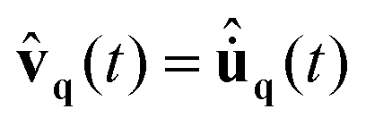 , its double Fourier transform satisfies the relation ṽq(ω) = iωũq(ω). By applying the time and space Fourier transform to eqn (4), we obtain the evolution of each Fourier mode of the displacement


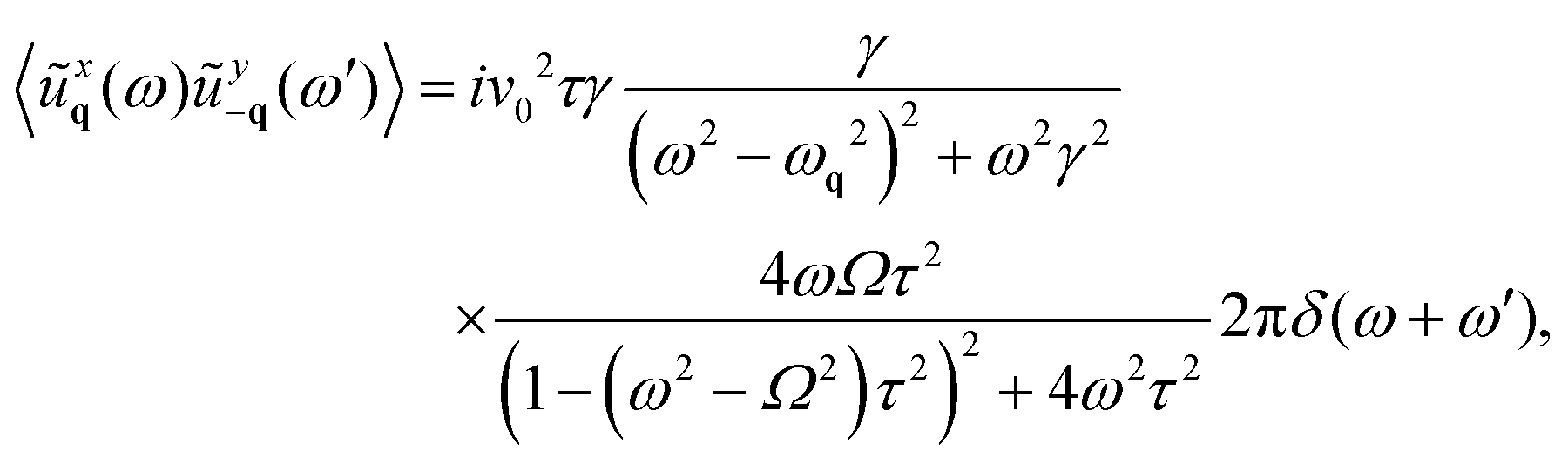
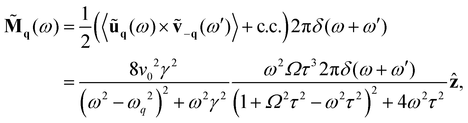


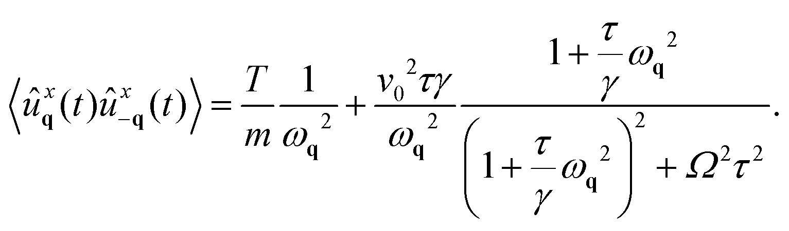
 , the active forces make a significant contribution to the correlations.
 , which upon converting the sums into integrals as in eqn (12), reads:
 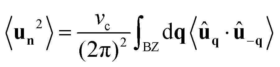 , where the integral, in principle, extends to the first Brillouin zone (BZ). However, in practice, we employ the Debye continuum approximation, which assumes a linear dispersion relation ∼q up to a maximum frequency, the Debye frequency. In this way, the lattice is treated as a continuous elastic medium, with a cutoff wavevector to match the number of allowed vibrational modes to the actual number of the lattice degrees of freedom. The model has the advantage of being mathematically straightforward and computationally efficient: it provides a reasonable approximation for low-frequency (long-wavelength) acoustic phonons where the linear dispersion relation is valid.
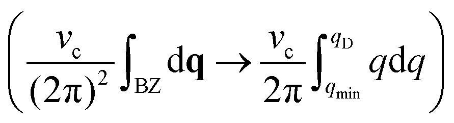 , with qmin = 2π/Na and qD = π/a. Since the integral is peaked near q = 0, we approximate the last fraction in eqn (13) as (1 + Ω2τ2)−1 and use the small-q approximation for ωq2 ≈ 3K/(2m)q2σ2 = c2q2, and obtain:
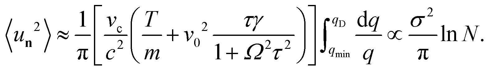
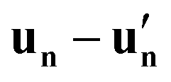 between any pair of sites (n and n′) exhibits only finite fluctuations if their separation is finite, indicating that local order is preserved. Notably, in active chiral systems, both the mean square displacement and
  are reduced compared to their values in the achiral case. This reduction occurs because the trajectories in systems with chirality (Ω ≠ 0) are curved, and the positional fluctuations are reduced by activity. This behavior is consistent with the dynamics of an active particle in a harmonic potential.48 The particle number density can be expressed as the sum of delta functions positioned at rn(t),
 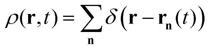 , where rn = Rn + un. Its Fourier transform, assuming 〈un〉 to be independent of the site index, reads:
 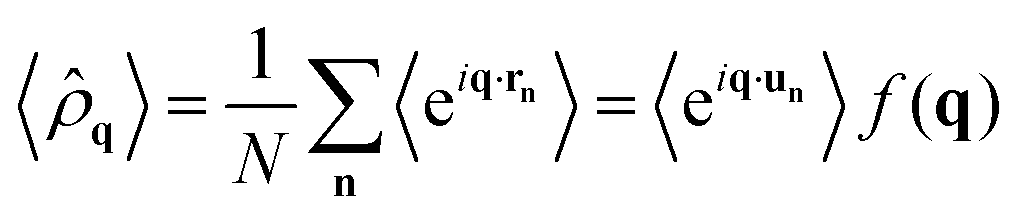 , where
  represents the Fourier transformed density of the frozen lattice. It is maximal when q = G, where G is a reciprocal wave-vector. Since the displacements have a Gaussian distribution, we write: 〈eiG·un〉 = e−〈(G·un)2〉/2 = e−WG. Thus, the Fourier components of the density associated with the reciprocal wave-vectors are 〈
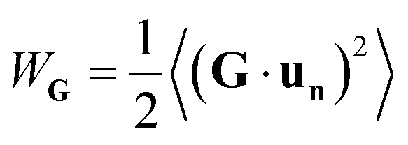 . Employing the approximate correlator and obtaining the following estimate:
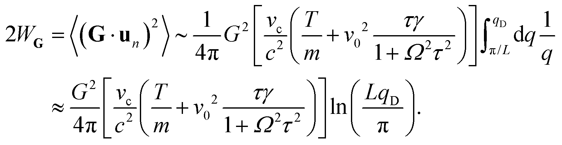

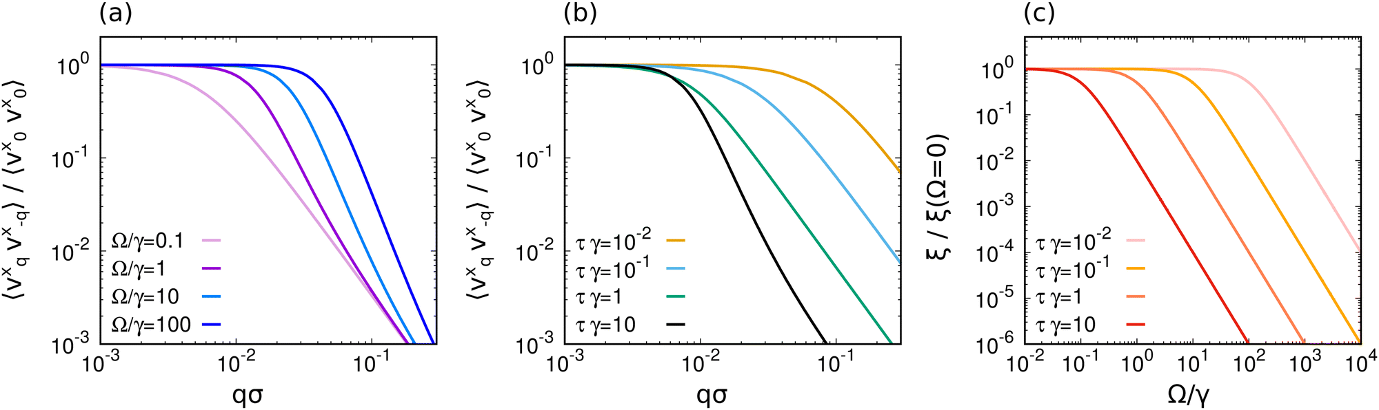
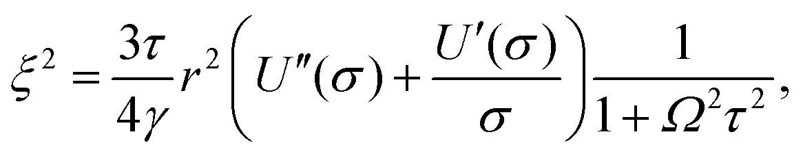


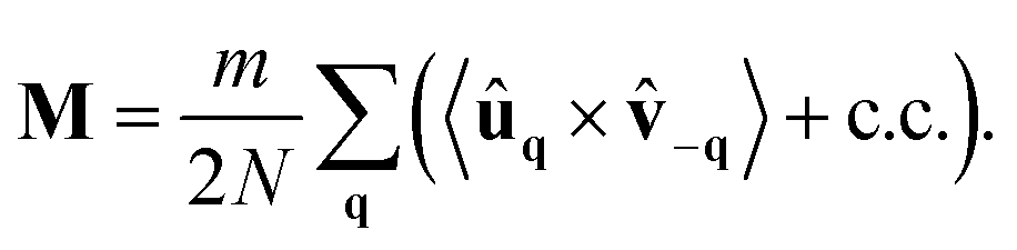
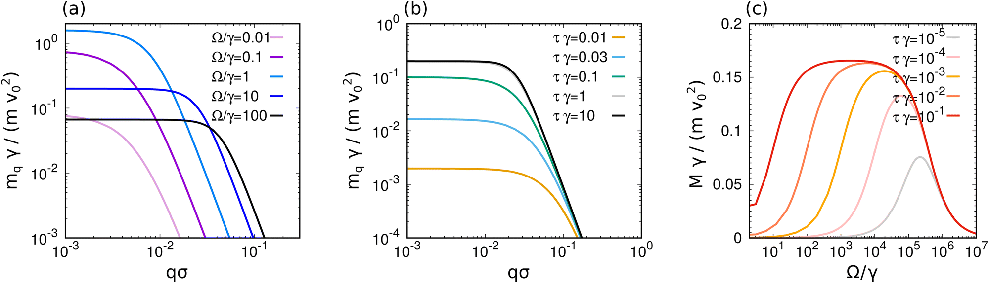
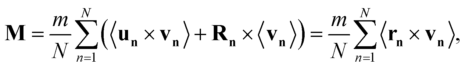

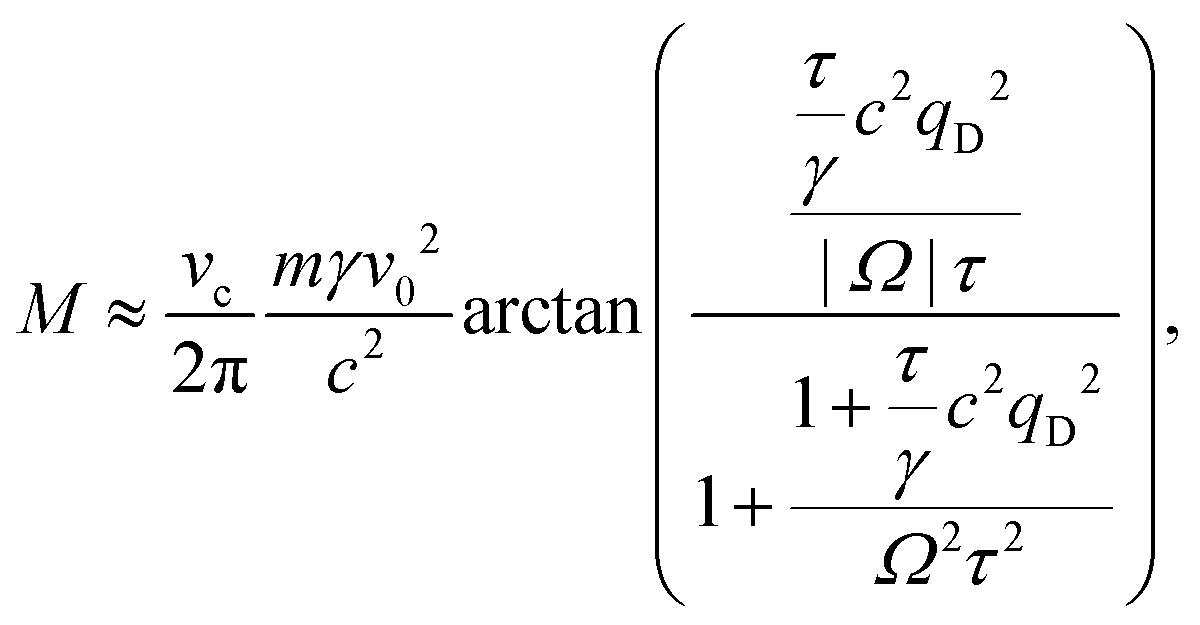
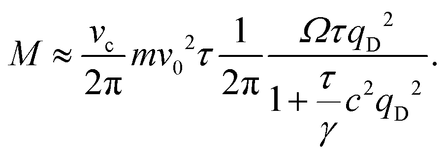
 . This results in a non-monotonic dependence on Ω which is evident for different values of τ as shown in Fig. 4(c). This non-monotonicity can be understood by noting that for Ω = 0 (in the absence of chirality) the angular momentum vanishes due to symmetry. Similarly, we expect M to vanish again for Ω → ∞. This behavior arises because chirality induces a bending of the trajectories of an active particle, thereby reducing displacement fluctuations compared to the non-chiral case, eventually suppressing them entirely for sufficiently large chirality. This interpretation aligns with the findings from the study of a single chiral active particle in a harmonic potential.48 Let us note that, as demonstrated in Appendix D, the torque, T, exerted by the active chiral forces on the particles is balanced by the torque exerted by the friction, the latter being proportional to the angular momentum multiplied the friction coefficient, γ, yielding: |T| = γM.
 , where a non-zero value of Ṡ differentiates non-equilibrium steady states from equilibrium states. It is worth noting that this expression is often referred to as the entropy production rate of the medium. However, this term coincides with the entropy production rate in the steady state, which is the primary focus of our interest.
 , and has the usual form of the entropy production rate of active particles, i.e. correspond to the work performed by the active force. The dependence on the chirality is implicitly contained in the equal-time correlations 〈fan(t)·vn(t)〉. Approximating this correlations, leads to the following result (see Appendix E)
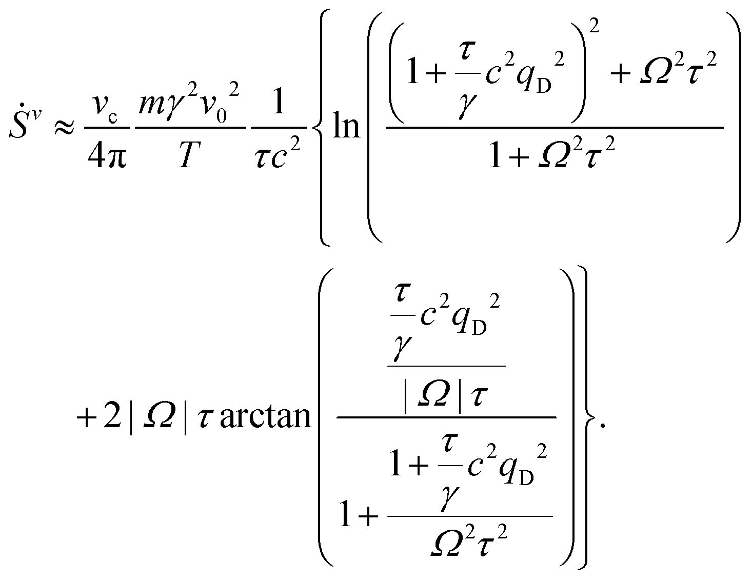

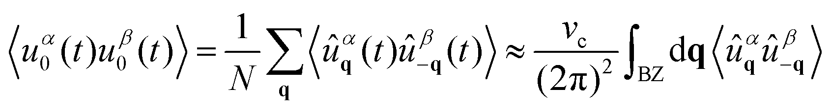


 . For time separations t exceeding τ, the most relevant terms in the correlations vary exponentially as
  , with slower decay for smaller wavevectors q. After a short initial transient, the amplitude of these long-wavelength modes contributes significantly to real-space correlations.
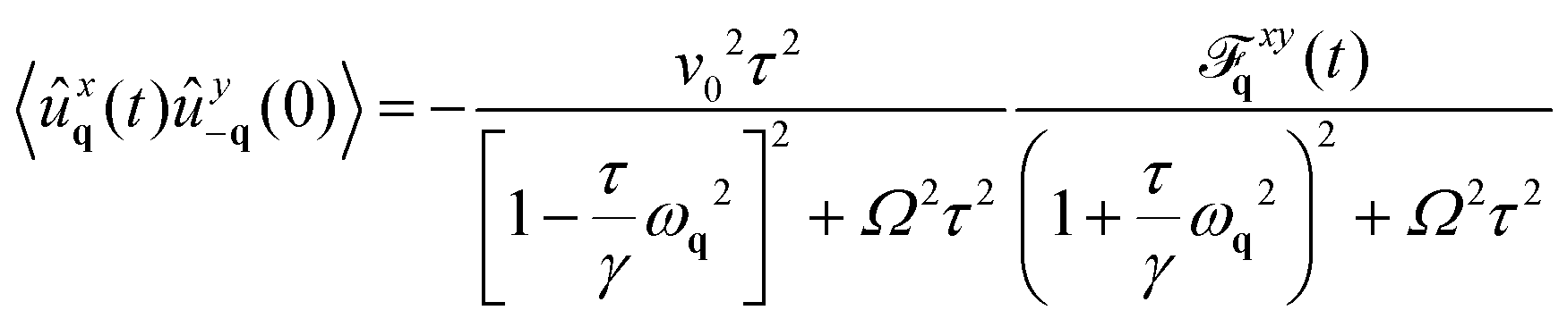

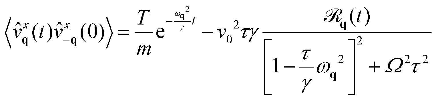
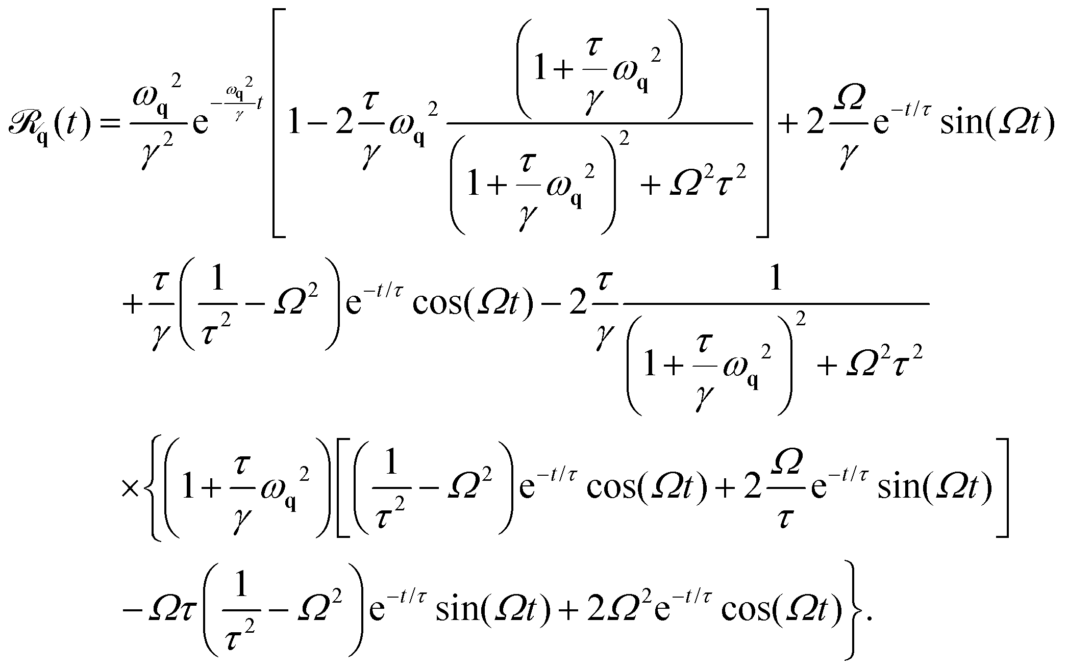


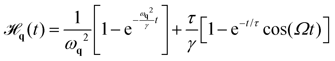
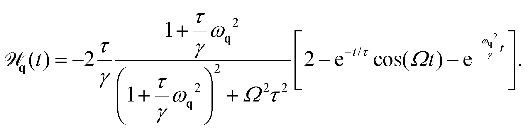
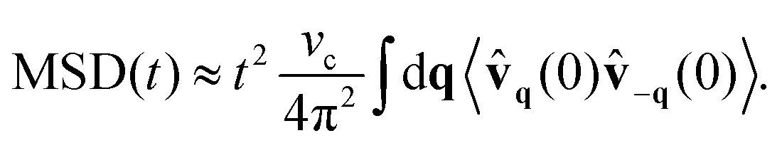


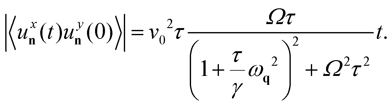
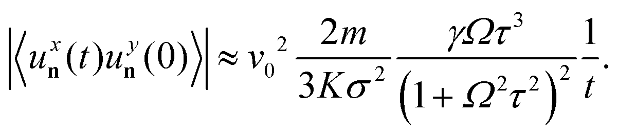

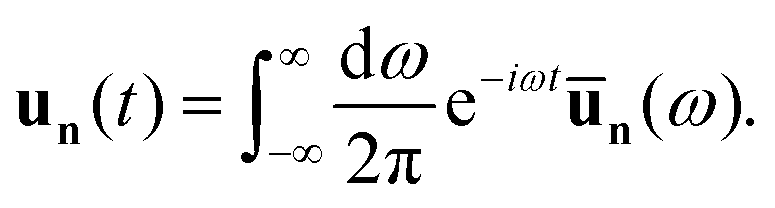
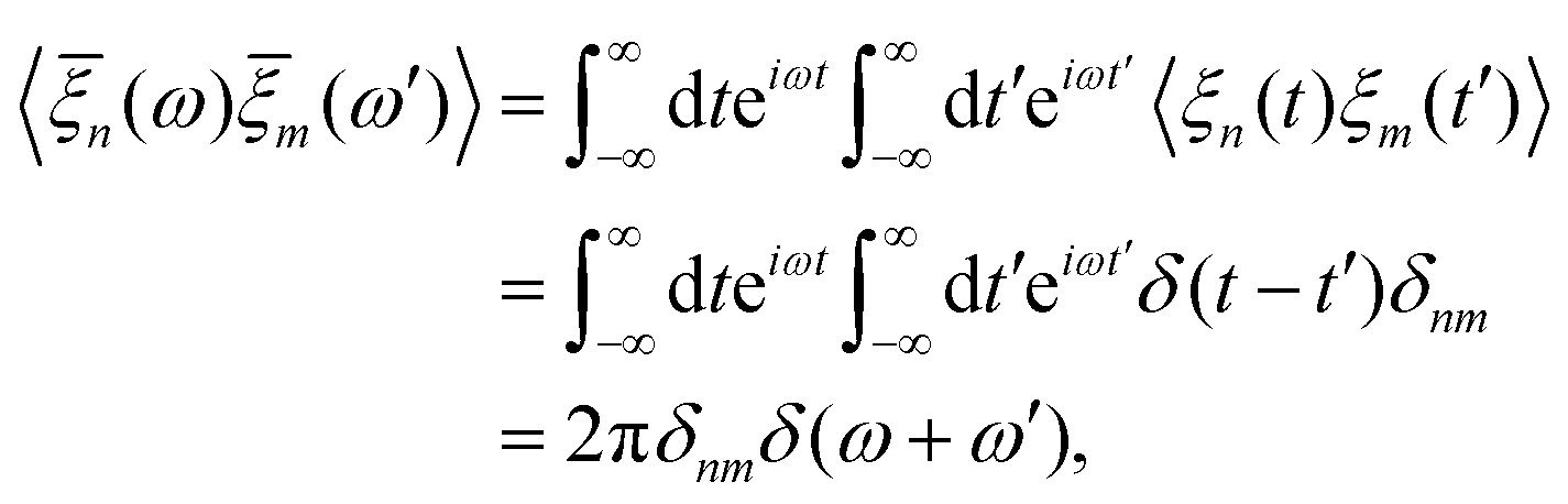
 . In a similar way, we can define the discrete spatial Fourier transform of the displacemente vector as
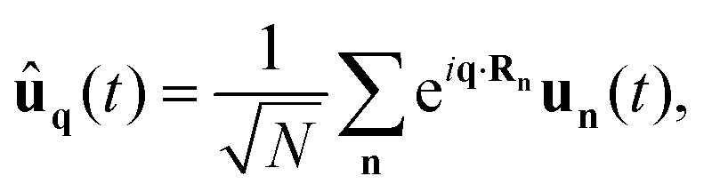


 via the propagator Ĝq(ω), introduced below eqn (6). We remark that the Fourier transforms of the white noises satisfy the following properties:
 .
.


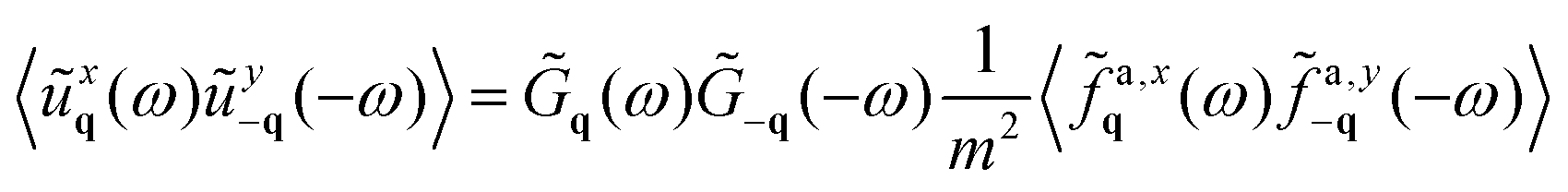


 and λ* is its complex conjugate. The solution of the overdamped eqn (70) is given by
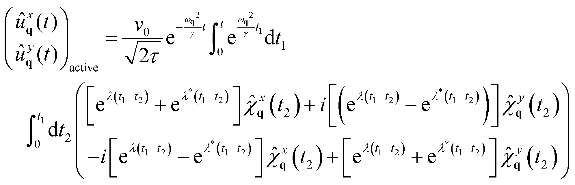


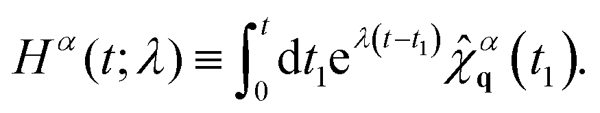
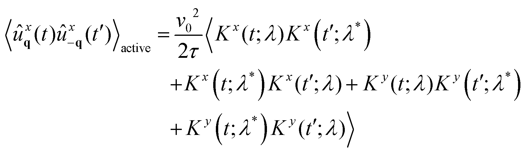
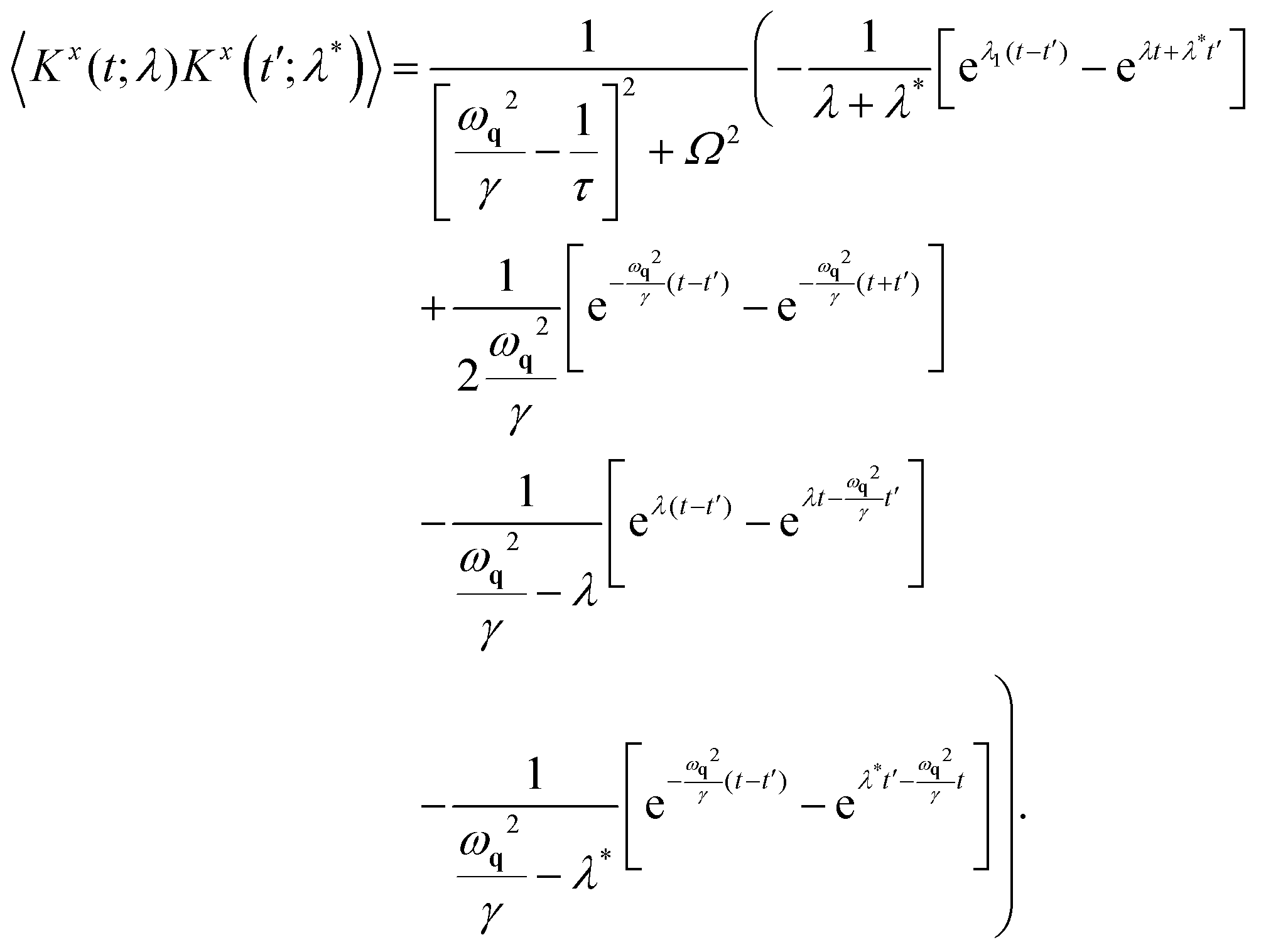


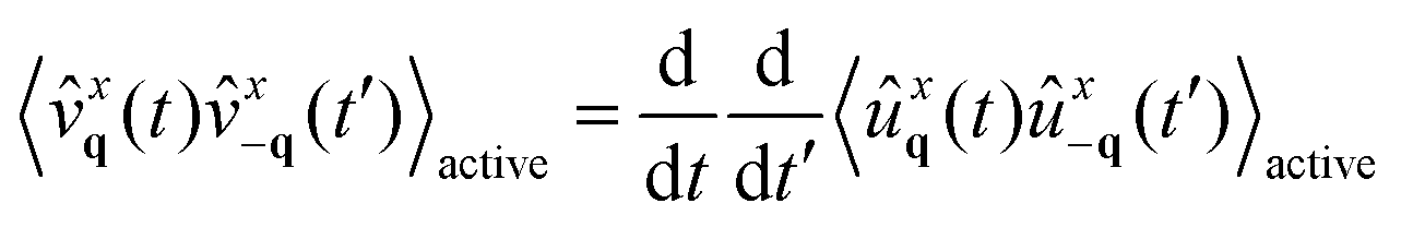


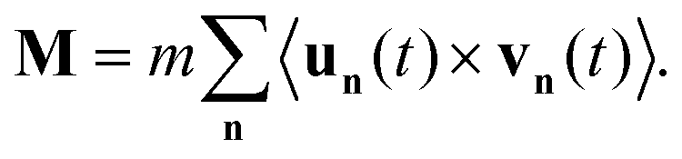
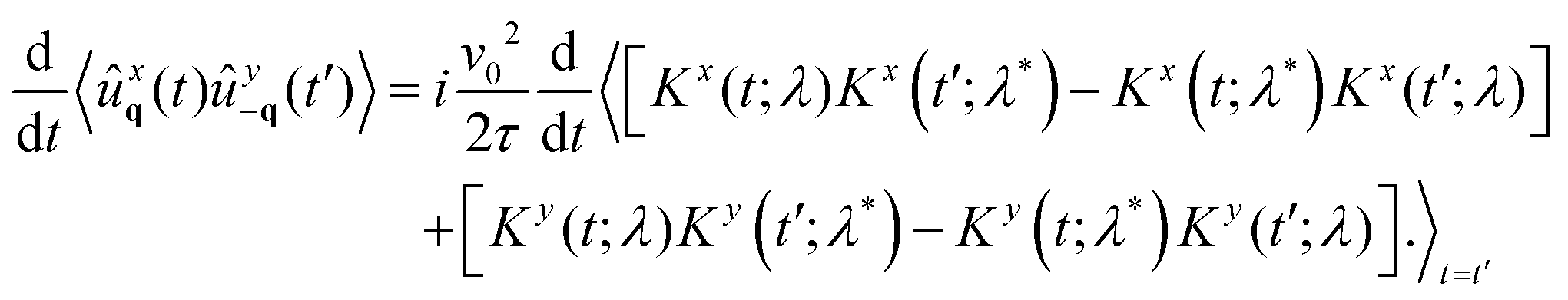

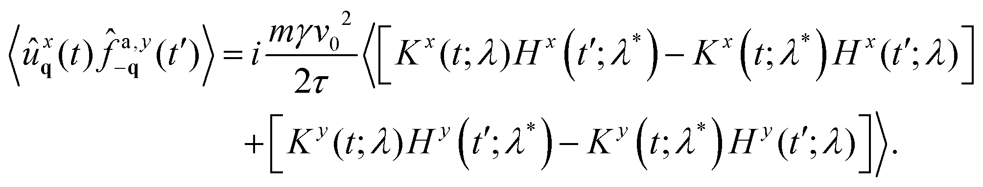
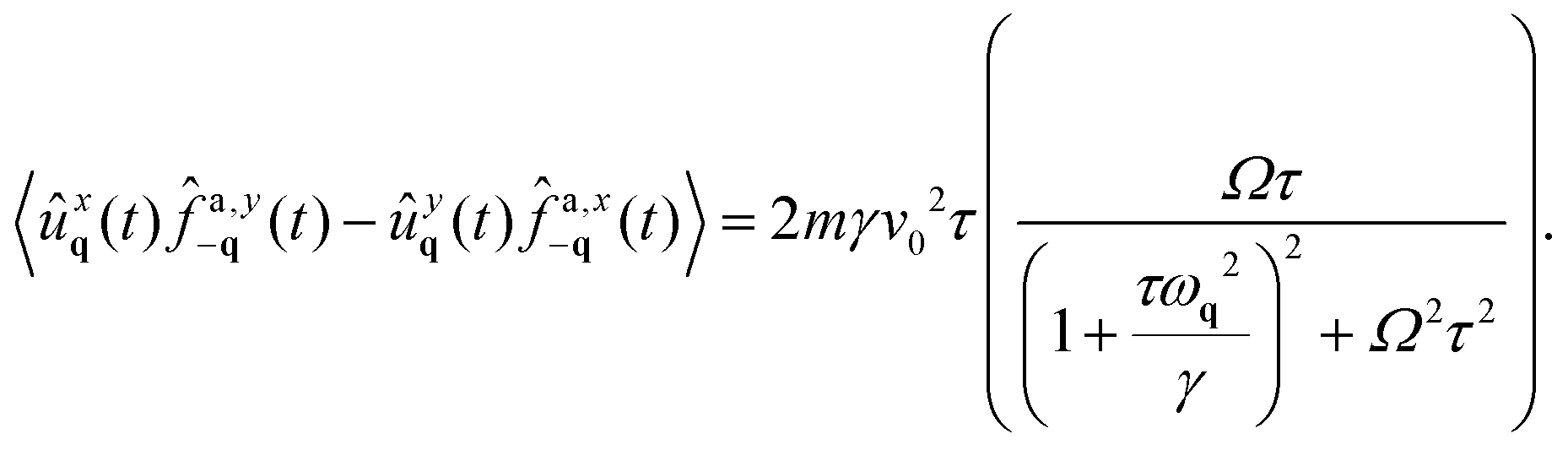

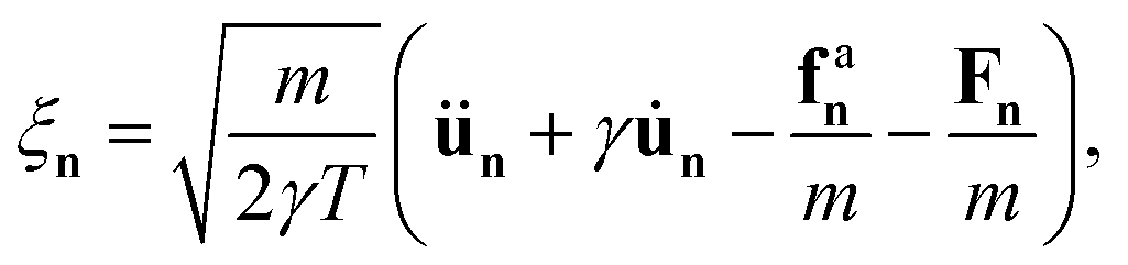


 in the achiral case, Ω = 0. The entropy rate production of the mode q is given by