 Open Access Article
Creative Commons Attribution 3.0 Unported Licence
Machine learning enhanced spectroscopic analysis: towards autonomous chemical mixture characterization for rapid process optimization†
Andrea
Angulo
 ,
Lankun
Yang
,
Eray S.
Aydil
and
Miguel A.
Modestino
,
Lankun
Yang
,
Eray S.
Aydil
and
Miguel A.
Modestino
 *
*
Department of Chemical and Biomolecular Engineering, Tandon School of Engineering, New York University, 6 Metroctech Ct., Brooklyn, NY 11201, USA. E-mail: modestino@nyu.edu
First published on 23rd December 2021
Abstract
Autonomous chemical process development and optimization methods use algorithms to explore the operating parameter space based on feedback from experimentally determined exit stream compositions. Measuring the compositions of multicomponent streams is challenging, requiring multiple analytical techniques to differentiate between similar chemical components in the mixture and determine their concentration. Herein, we describe a universal analytical methodology based on multitarget regression machine learning (ML) models to rapidly determine chemical mixtures' compositions from Fourier transform infrared (FTIR) absorption spectra. Specifically, we used simulated FTIR spectra for up to 6 components in water and tested seven different ML algorithms to develop the methodology. All algorithms resulted in regression models with mean absolute errors (MAE) between 0–0.27 wt%. We validated the methodology with experimental data obtained on mixtures prepared using a network of programmable pumps in line with an FTIR transmission flow cell. ML models were trained using experimental data and evaluated for mixtures of up to 4-components with similar chemical structures, including alcohols (i.e., glycerol, isopropanol, and 1-butanol) and nitriles (i.e., acrylonitrile, adiponitrile, and propionitrile). Linear regression models predicted concentrations with coefficients of determination, R2, between 0.955 and 0.986, while artificial neural network models showed a slightly lower accuracy, with R2 between 0.854 and 0.977. These R2 correspond to MAEs of 0.28–0.52 wt% for mixtures with component concentrations between 4–10 wt%. Thus, we demonstrate that ML models can accurately determine the compositions of multicomponent mixtures of similar species, enhancing spectroscopic chemical quantification for use in autonomous, fast process development and optimization.
1. Introduction
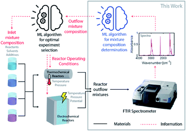
Driven by an exponential increase in computational power and the ability to collect, store, and process massive amounts of data, machine learning (ML) has emerged as an invaluable tool for amplifying the performance of many technologies and businesses ranging from self-driving vehicles, targeted marketing, medical diagnostics to financial market forecasting. During the last three years, several studies implemented ML for automating and accelerating chemical process discovery, development, and optimization at the laboratory scale with impressive results,1–8 but ML has not been fully exploited in this context. Advances on this front can have an enormous impact on chemical manufacturing.The ML approaches used for chemical process development generally rely on a feedback loop between (1) an ML-guided high-throughput experimental system featuring a chemical reactor and (2) an analytic tool to determine the compositions of the process outlet streams (Fig. 1). Within this approach, an ML algorithm selects optimal experimental conditions to test (e.g., inlet mixture composition, reactor operating conditions), which are then implemented in a reactor (e.g., thermochemical or electrochemical) by an autonomous and automated system. The outlet streams from the reactors, containing mixtures of the desired chemicals byproducts, solvents, additives, and unreacted precursors, are characterized by an analytical tool to determine their composition and the initial ML algorithm uses this information to select the next set of experiments. Determining the composition of an unknown chemical mixture is a challenging task that requires a suite of analytical tools with varying costs and speed (e.g., nuclear magnetic resonance, liquid and/or gas chromatography, mass spectrometry, and/or various optical spectroscopies, amongst others). Moreover, each technique or combination must be adapted to the chemical mixture of interest to provide complete compositional information.
An autonomous chemical process optimization system such as that depicted in Fig. 1 would ideally use a generally applicable, non-invasive, fast, and inexpensive spectrochemical characterization tool capable of quantifying the compositions of multicomponent mixtures based on unique identifying molecular spectral features. However, interpretation of spectra collected from mixtures can be complex, and their interpretation and quantification are often challenging because of spectral feature overlap and interactions between different species. We address this challenge in this study by developing and demonstrating a universal ML algorithm that enables rapid inline mixture characterization using an inexpensive Fourier transform infrared (FTIR) spectrometer. The approach we describe is particularly well suited for organic synthesis and aqueous molecular solutions comprising chemicals with vibrational fingerprints, a significant fraction of cases of interest.
FTIR spectroscopy is one of the most powerful and widespread analytical techniques to determine the presence of functional groups in molecules, the compositions of chemical solutions, and to study chemical processes inline or in situ.9 FTIR-based methods often rely on the characterization of the position or absorbance of only a few spectroscopic features (absorption peaks) that are indicative of functional groups, while a large fraction of the spectra is ignored because overlapping features are difficult to discern, especially in the fingerprint region (i.e., ∼400–1500 cm−1). Furthermore, when multiple analytes are present in the solution, absorption peaks from different molecules can overlap, and interactions between molecules can cause shifts in their positions, significantly increasing the complexity of the analysis.10
Machine learning (ML) algorithms can enhance humans' ability to extract information from complex spectral data by learning the correlations between mixture compositions and absorption features. Such algorithms and FTIR data have already been used in specific food and materials applications.10–12 Previous studies have applied active learning to train classification algorithms and then use these algorithms to identify specific molecules in mixtures.13–15 A few studies have used regression algorithms to determine species concentrations.16,17 Recent examples of ML-enhanced FTIR analysis include the use of support vector machine (SVM) classifiers for rapid identification and quantification of components in artificial sweeteners with a prediction accuracy ranging between 60–94%,17 and the use of linear regression to determine electrolyte composition in lithium-ion batteries within an absolute error of 3–5 wt%.18 In the first case, the ML models were trained using only 131 absorbance points at selected wavenumbers, and the methodology included spectroscopy preprocessing methods (Savitzky–Golay, first derivative, and their combination). In the second, the ML methodology included multiple data preprocessing steps and manual selection of IR regions for specific functional groups pertaining to the species of interest. In both cases, the sample preparation was done by a lab operator.
Currently, there are multiple open-source and commercial software tools available that can facilitate the implementation of ML algorithms. These tools include MATLAB® PLS Toolbox software and Python's ScikitLearn, Keras, TensorFlow open-source library, among others.
Inspired by the successful implementation of ML in these specific applications, we developed a universal algorithm that uses supervised ML models to determine the concentrations of chemical species in solutions via multitarget regression with minimal human intervention. We first generate multicomponent mixture FTIR spectra by linearly combining pure species spectra using the respective molar fractions of each component as weights. These simulated multicomponent spectra are then used to train ML algorithms and develop an ML methodology to determine the compositions of real chemical mixtures. Finally, the ML algorithms are validated and evaluated by comparing their predictions of the compositions of experimental mixtures from their measured FTIR spectra. We used the reactants and possible products of two chemical reactions as model mixture components: electroreduction of acrylonitrile (AN) to adiponitrile (ADN), a nylon precursor, and the valorization of glycerol into other high-value C3 products. We found that Artificial Neural Networks (ANN) and Linear Regression (LR) with Principal Component Analysis (PCA), also known as Principal Component Regressor (PCR), lead to the most accurate predictions, with R2 values ranging between 0.854–0.986 and mean absolute errors (MAE) between 0.28–0.52 wt%, depending on the number and identity of components, and ML algorithm.
2. Results and discussion
2.1. Machine learning methodology development
To develop a robust ML approach, we evaluated the performance of various models using the absorbance (A.U.) at n different wavenumbers (wn), Ā = [A1,…,An], as predictor variables, and the concentrations of all (m of them) mixture components,![[C with combining macron]](https://www.rsc.org/images/entities/i_char_0043_0304.gif) = [C1,…,Cm] as target variables. Both n and m can vary based on the spectrometer resolution and the number of mixture components, respectively. As a model system, we first considered mixtures of up to 6 components with similar absorption features and relevant to the electrochemical production of nylon precursors: acrylonitrile (AN), adiponitrile (ADN), propionitrile (PN), ethylenediaminetetraacetic acid (EDTA), phosphate ions (PO43−) and tetramethylammonium ions (TMA), in aqueous solutions.19 The individual spectra of each one of these components are shown in Fig. 2. Mixture FTIR spectra were generated by linearly combining pure species spectra according to Beer's law,
= [C1,…,Cm] as target variables. Both n and m can vary based on the spectrometer resolution and the number of mixture components, respectively. As a model system, we first considered mixtures of up to 6 components with similar absorption features and relevant to the electrochemical production of nylon precursors: acrylonitrile (AN), adiponitrile (ADN), propionitrile (PN), ethylenediaminetetraacetic acid (EDTA), phosphate ions (PO43−) and tetramethylammonium ions (TMA), in aqueous solutions.19 The individual spectra of each one of these components are shown in Fig. 2. Mixture FTIR spectra were generated by linearly combining pure species spectra according to Beer's law, | (1) |
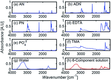 | ||
| Fig. 2 (a–g) The FTIR absorption spectra of pure components. (h) The spectrum resulting from a linear combination of spectra in (a–g), using a molar concentration of 0.05% for each component. | ||
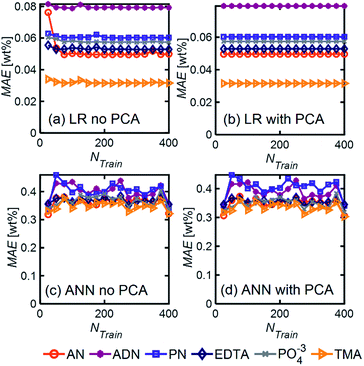
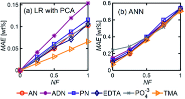
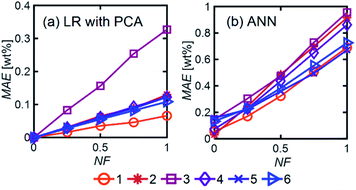
Even in the presence of significant noise, LR performed better than ANN, with a smaller MAE between a factor of 5–10, depending on the component of interest. In LR models, TMA had the lowest MAE, which can be attributed to the substantial differences between its spectrum and other components in the range of 4000–1000 cm−1, which results in a simpler differentiation. On the other hand, ADN concentration has the highest MAE given its multiple overlapping peaks with PN and AN and the lower magnitude of the peaks in the fingerprint region, which are more severely affected by noise.
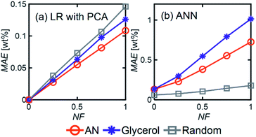
LR MAE as a function of NF behaved similarly for all three types of mixtures, but for ANN, the MAE of the models for the random mixture outperformed the other two, especially at high noise levels (Fig. 8). This is likely because random molecules do not necessarily have similar functional groups (fewer overlapping characteristic peaks), which makes it easier for the algorithm to differentiate between them.
2.2. Experimental implementation of ML methodology
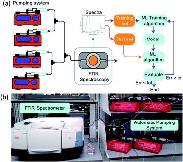
To systematically collect spectra for training the ML models, we used a network of programmable pumps that flowed solutions of selected components with known concentrations into a transmission FTIR flow cell (Fig. 9). A deionized water background was used as a reference. Based on the programmed flowrates and the spectral measurements, we collected ∼50 labelled spectra per day, which were then used to obtain LR or ANN regression models. The ML models were developed by partitioning the data randomly into training and testing sets, applying PCA, and then evaluating their performance using the prediction accuracy for the test set. This process was repeated, and new hyperparameters were determined at each iteration until the error was lower than a set tolerance or until the performance stopped improving. The absorbance values at each wn were used as the predictors, and mass concentrations (in wt%) were used as the predictions. The absorbance data range was limited to between 3000 and 1000 cm−1 because absorption saturated outside of this range.This methodology allowed for the collection of 50 data points per day. An operator was in charge of collecting and labelling samples and refilling the syringes with the single component solutions once they were depleted. This methodology allowed for the autonomous collection of at least 50 data points per day, with human intervention only required to fill the syringes with single component solutions initially. This methodology also allows us to use entire IR spectral measurement as input for our ML models, without needing to select characteristic absorption regions and circumvents the problem of overlapping features of classical approaches.
Fig. 10 shows selected FTIR spectra of 3-component mixtures with different compositions. The spectra look similar to the eye, with subtle changes in the intensities of some peaks. Without ML models here, one would have to carefully identify peaks for each species, correct for baseline, deconvolute and fit peaks, a nontrivial and arduous task to determine mixture compositions.
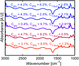 | ||
| Fig. 10 FTIR spectral measurements for glycerol (gly), isopropanol (IPA), and 1-butanol (1-but) mixtures at different mass concentrations, Cgly, CIPA, C1-but, respectively. | ||
We show, however, that ML models with PCA can determine unknown compositions from spectra similar to these. We studied five different aqueous solutions differing in numbers and types of components in the mixture. Table 1 shows the species in the aqueous solution for each of the cases studied.
| Mixture label | Species | Number of PC selected | Experimental spectra collected |
|---|---|---|---|
| 1-Gly | Glycerol | 2 | 30 |
| 2-AN | AN, ADN | 3 | 50 |
| 3-Gly | Glycerol, IPA, 1-butanol | 5 | 109 |
| 3-AN | AN, ADN, PN | 5 | 67 |
| 4-AN | AN, ADN, PN, glycerol | 7 | 50 |
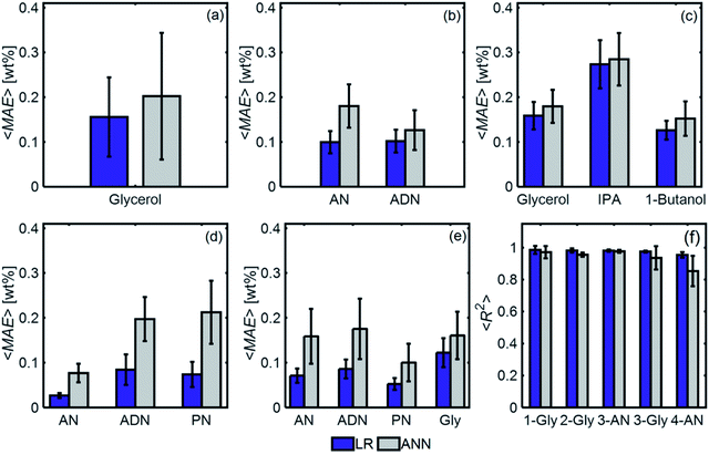
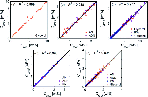
Fig. 11 compares the performances of LR implemented with PCA and ANN for the mixtures in Table 1. The 〈MAE〉 of the concentrations predicted [wt%] ranged from 0.023% to 0.28%. The 〈MAE〉 for glycerol-based mixtures did not significantly change between 1-component and 4-component mixtures. The 〈R2〉 values varied between 0.854 and 0.986, decreasing as the number of components increased. LR models had higher accuracy and weaker dependence on train/test subset combinations than ANN models for all mixtures. Fig. 12 shows the predicted and actual concentrations for the mixtures in Table 1. The subplots in this figure depict a model trained with a randomly chosen subset of the entire spectral data set, while the results in Fig. 11 show 〈MAE〉 averaged over 200 models.
3. Conclusions
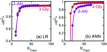
We described a general methodology for developing and implementing ML models for quantitatively predicting chemical mixture compositions from their FTIR spectra. For model mixtures chosen from practical applications, we trained linear regression (LR) and artificial neural network (ANN) models with R2 regression scores ranging from 0.98 to 0.99 and 0.94 to 0.98, respectively. Simpler and less computationally expensive linear regression models were consistently more accurate than ANN models, making them a superior choice for quantitative composition prediction from FTIR spectra. We also studied the relationship between model performance and the number of spectra in the training data set and found that for both LR and ANN, regression scores increased and saturated at approximately 40 spectra for 3-component mixtures. Finally, we showed that trained ML models (Linear Regression with PCA and Neural Networks) maintain their accuracy despite small variations in experimental conditions expected over several days. Our results suggest that this methodology can enhance the analytical capabilities of FTIR spectroscopy for quantitative composition determination and find applications in inline chemical analysis applications that require fast characterization, such as autonomous chemical process development and optimization.4. Experimental methods
4.1. Materials
Acrylonitrile (AN), adiponitrile (ADN), propionitrile (PN), 1-butanol, and glycerol were purchased from Sigma Aldrich. Isopropanol 70% was purchase from VWR. Stock solutions were prepared with deionized (DI) water.The pumping system consisted of two NE-1000 Programmable Syringe Pumps and two NE-4000 Programmable 2-Channel Syringe Pumps, manufactured by New Era Pump Systems: 60 ml and 30 ml BD syringes were used to load the stock solutions into the system. A Nicolet iS50 FTIR Spectrometer and OMNIC software were used for spectral data collection. The transmission flow cell was purchased from Harrick Scientific Products and consisted of a demountable liquid cell with Luer lock fittings and a 20 mm diameter clear aperture, equipped with a pair of 25 mm diameter ZnSe transmission windows. For all experiments, the spacing between the transmission windows was 12 μm.
4.2. Simulated data generation
Simulated spectral data for mixtures of selected components were generated using Beer's law (eqn (1)). For the training set, a concentration matrix,![[C with combining macron]](https://www.rsc.org/images/entities/i_char_0043_0304.gif) , with dimensions p × (n + 1), where p is the number of points to generate, and n is the number of different components to consider, was generated according to a Sobol sequence.23 For the test set, a concentration matrix was created based on random distribution sampling. Compositions of individual solutes were maintained below 10% with water as a solvent. Applying a dot product between
, with dimensions p × (n + 1), where p is the number of points to generate, and n is the number of different components to consider, was generated according to a Sobol sequence.23 For the test set, a concentration matrix was created based on random distribution sampling. Compositions of individual solutes were maintained below 10% with water as a solvent. Applying a dot product between ![[C with combining macron]](https://www.rsc.org/images/entities/i_char_0043_0304.gif) and a vertically concatenated matrix of the spectral data of the individual components Āpure, results in a matrix of spectra, S, where each row is a new spectrum corresponding to a mixture of known concentrations.
and a vertically concatenated matrix of the spectral data of the individual components Āpure, results in a matrix of spectra, S, where each row is a new spectrum corresponding to a mixture of known concentrations.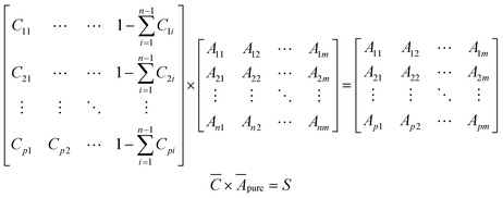 | (2) |
4.3. Simulated noise introduction
To introduce noise to the simulated test data, we defined a variable noise factor, NF, ranging from 0 (no noise assigned) to 1 (maximum noise-to-signal ratio). A number between −0.05 and +0.05 A.U. was randomly selected, multiplied by NF, and then added to each absorbance point of a spectrum. The noise range was selected based on the difference observed between the FTIR spectrum obtained from spectral libraries and the spectrum of a glycerol sample collected experimentally in our equipment using only five scans. Fig. 14 shows sample spectra at three different NF levels for an aqueous solution containing AN, ADN, and PN.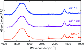 | ||
| Fig. 14 Illustration of simulated noise introduction to spectra at three different NF levels for an aqueous solution containing AN, ADN, and PN. | ||
4.4. Data preprocessing: principal component analysis
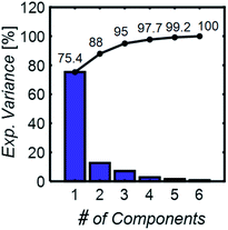
Principal component analysis (PCA) was used as a dimensionality reduction technique to decrease the number of spectral data points from thousands to up to 10 principal components for the studies conducted with simulated and experimental data. The number of principal components selected depended on the number of chemical components in the solution under study. PCA was implemented using the sklearn.preprocessing.PCA() function from scikit-learn, an ML library for Python.244.5. Machine learning algorithm training and evaluation
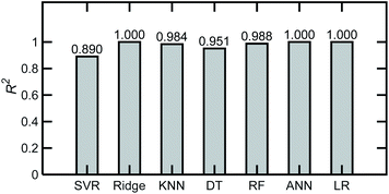
Machine learning models were developed to describe relationships between solution compositions and their FTIR absorbance spectra. Different ML regression algorithms available in the scikit-learn library were initially evaluated for a base case comprising 200 simulated spectra of tertiary mixtures in water, with an NF = 0. The algorithms and respective scikit-learn functions are described in Table 2.| Model | Function |
|---|---|
| Linear regression (LR) | sklearn.linear_model |
| Multilayer perceptron regression or artificial neural networks (ANN) | sklearn.neural_network.MLPRegressor |
| Decision trees | sklearn.tree.DecisionTreeRegressor |
| Random forests (RF) | sklearn.ensemble.RandomForestRegressor |
| Support vector regressor (SVR) | sklearn.svm.SVR |
| Ridge regression with cross validation (RidgeCV) | sklearn.linear_model.RidgeCV |
| k-Nearest neighbors (kNN) | sklearn.neighbors.KNeighborsRegressor |
Hyperparameters were optimized using sklearn.model_selection.RandomizedSearchCV. When developing regression models, the predictors or features were the absorbance values at each wavenumber, a matrix denoted S, and the target or predicted variables were the concentrations corresponding to each spectrum, contained in a concentration vector (for 1-component solution) or matrix (for a multicomponent solution) denoted C. For the experimentally collected data, S and C were divided randomly into a training and a test set, with a training![[thin space (1/6-em)]](https://www.rsc.org/images/entities/char_2009.gif) :
:![[thin space (1/6-em)]](https://www.rsc.org/images/entities/char_2009.gif) test ratio of 80
test ratio of 80![[thin space (1/6-em)]](https://www.rsc.org/images/entities/char_2009.gif) :
:![[thin space (1/6-em)]](https://www.rsc.org/images/entities/char_2009.gif) 20%. To avoid model performance dependency on the random training to test partition, each study was repeated 200 times, after which the average metrics were calculated and reported. The infrared wavenumber range for the simulated and experimental data were 4000–1000 cm−1 and 3000–1000 cm−1, respectively, the latter omitting the 4000–3000 cm−1 range where the noise is very high due to nearly complete absorption by the water O–H stretching vibration.
20%. To avoid model performance dependency on the random training to test partition, each study was repeated 200 times, after which the average metrics were calculated and reported. The infrared wavenumber range for the simulated and experimental data were 4000–1000 cm−1 and 3000–1000 cm−1, respectively, the latter omitting the 4000–3000 cm−1 range where the noise is very high due to nearly complete absorption by the water O–H stretching vibration.
Fig. 15 summarizes the general approach for developing ML regression models for the simulated and the experimentally collected data.
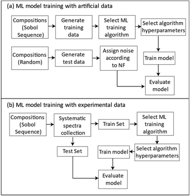 | ||
| Fig. 15 A flowchart for the general approach to ML model development with (a) simulated generated and (b) experimentally collected data. | ||
4.6. FTIR experimental data collection
Spectral measurements of mixtures of known concentrations were pumped into a transmission flow cell placed inside the FTIR spectrometer using a network of programmable pumps, each loaded with a single component aqueous stock solution. Concentrations of the mixture flowing through the cell were changed and controlled by varying the flow rates of the individual single-component solutions. The pumps were programmed to switch flow rates periodically at set intervals, allowing for automated spectra collection while varying compositions. For a two-component mixture, the total flow rates were maintained at 1 ml min−1, 1.5 ml min−1, and 2 ml min−1 for two-, three- and four-component mixtures, respectively. The set of compositions to sample were determined using a Sobol sequence. New sampling intervals were determined every time a new component was introduced by pumping a new solution into the flow cell and periodically taking spectral measurements until the resulting spectrum stopped changing over time. All spectra were taken with respect to the water background. Deionized water background was recorded only once at the beginning of each sampling collection session, which typically lasted for about 6 hours at the most. Datasets for one type of mixture were collected during 4 days (3-gly). Performance for the 3-gly mixtures specifically was 0.982 and 0.977 for LR and ANN, which suggests that the same model can be used for experimental campaigns that span several days without the need for recalibration.The set of compositions to sample were determined using a Sobol sequence.
The code and data for simulated noise generation and introduction, data preprocessing, machine learning algorithm training and evaluation and collected FTIR spectral data are available in a public repository.25
Data availability
(1) The code for machine learning regression models development, both for synthetic and experimental data, can be found at https://doi.org/10.5281/zenodo.5498197 with 10.5281/zenodo.5498197. The version of the code employed for this study is version V1.0.0. (2) Data for the generation of the Machine Learning Regression Models, including.csv files for the experimentally collected data for chemical mixtures of known concentration, as well as the corresponding labels, are available at 10.5281/zenodo.5498197 at https://doi.org/10.5281/zenodo.5498197.Author contributions
The manuscript was written through the contributions of all authors. All authors have approved the final version of the manuscript. Andrea Angulo and Lankun Yang performed the experimental measurements. Andrea Angulo developed the Machine Learning methodology. Eray Aydil and Miguel Modestino conceptualized this work.Conflicts of interest
MAM is a director and has a financial interest in Sunthetics, Inc., a start-up company in the chemical process optimization space. New York University intends to pursue intellectual property protection for parts of the material presented in this work.Acknowledgements
The authors acknowledge the financial support provided by the National Science Foundation (Grant # CBET-1943972) and from NYU, Tandon School of Engineering, through the MAM and ESA startup funds. In addition, the collaboration between MAM and ESA is enabled by the Center for Decarbonizing Chemical Manufacturing Using Electrification (DC-MUSE), formed with the help of a generous grant from the Sloan Foundation (Grant # 201-16807) and a center planning grant from the National Science Foundation (Grant # EEC-1936709).Notes and references
- F. Häse, L. M. Roch and A. Aspuru-Guzik, Trends Chem., 2019, 1, 282–291 CrossRef.
- C. W. Coley, N. S. Eyke and K. F. Jensen, Angew. Chem., Int. Ed., 2020, 59, 22858–22893 CrossRef CAS.
- Z. Zhou, X. Li and R. N. Zare, ACS Cent. Sci., 2017, 3, 1337–1344 CrossRef CAS PubMed.
- A.-C. Bédard, A. Adamo, K. C. Aroh, M. G. Russell, A. A. Bedermann, J. Torosian, B. Yue, K. F. Jensen and T. F. Jamison, Science, 2018, 361, 1220–1225 CrossRef PubMed.
- B. J. Shields, J. Stevens, J. Li, M. Parasram, F. Damani, J. I. M. Alvarado, J. M. Janey, R. P. Adams and A. G. Doyle, Nature, 2021, 590, 89–96 CrossRef CAS.
- B. Burger, P. M. Maffettone, V. V. Gusev, C. M. Aitchison, Y. Bai, X. Wang, X. Li, B. M. Alston, B. Li, R. Clowes, N. Rankin, B. Harris, R. S. Sprick and A. I. Cooper, Nature, 2020, 583, 237–241 CrossRef CAS PubMed.
- M. Christensen, L. P. E. Yunker, F. Adedeji, F. Häse, L. M. Roch, T. Gensch, G. dos Passos Gomes, T. Zepel, M. S. Sigman, A. Aspuru-Guzik and J. E. Hein, Commun. Chem., 2021, 4, 112 CrossRef.
- D. E. Blanco, B. Lee and M. A. Modestino, Proc. Natl. Acad. Sci. U. S. A., 2019, 116, 17683–17689 CrossRef CAS PubMed.
- C. Berthomieu and R. Hienerwadel, Photosynth. Res., 2009, 101, 157–170 CrossRef CAS PubMed.
- S. Kern, S. Liehr, L. Wander, M. Bornemann-Pfeiffer, S. Müller, M. Maiwald and S. Kowarik, Anal. Bioanal. Chem., 2020, 412(18), 4447–4459 CrossRef CAS PubMed.
- F. Lussier, V. Thibault, B. Charron, G. Q. Wallace and J.-F. Masson, TrAC, Trends Anal. Chem., 2020, 124, 115796 CrossRef CAS.
- S. Kiyohara, M. Tsubaki, K. Liao and T. Mizoguchi, J. Phys.: Mater., 2019, 2, 024003 CAS.
- M. M. Y. R. Riad, Y. M. Sabry and D. Khalil, 2019 36th National Radio Science Conference (NRSC), 2019, pp. 386–392 Search PubMed.
- E. Bona, I. Marquetti, J. V. Link, G. Y. F. Makimori, V. da Costa Arca, A. L. G. Lemes, J. M. G. Ferreira, M. B. dos Santos Scholz, P. Valderrama and R. J. Poppi, LWT--Food Sci. Technol., 2017, 76, 330–336 CrossRef CAS.
- Y. Liu, F. Wang, C. Shao, W. You and Q. Chen, in International Conference on Mechatronics and Intelligent Robotics, 2019, vol. 856, pp. 784–791 Search PubMed.
- N. Zimmerman, A. A. Presto, S. P. N. Kumar, J. Gu, A. Hauryliuk, E. S. Robinson, A. L. Robinson and R. Subramanian, Atmos. Meas. Tech., 2018, 11, 291–313 CrossRef.
- Y.-T. Wang, B. Li, X.-J. Xu, H.-B. Ren, J.-Y. Yin, H. Zhu and Y.-H. Zhang, Food Chem., 2020, 303, 125404 CrossRef CAS.
- L. D. Ellis, S. Buteau, S. G. Hames, L. M. Thompson, D. S. Hall and J. R. Dahn, J. Electrochem. Soc., 2018, 165, A256–A262 CrossRef CAS.
- D. E. Blanco and M. A. Modestino, Trends Chem., 2019, 1, 8–10 CrossRef CAS.
- T. G. Mayerhöfer and J. Popp, Appl. Spectrosc., 2020, 74(10), 1287–1294 CrossRef PubMed.
- M.-L. O’Connell, A. G. Ryder, M. N. Leger and T. Howley, Appl. Spectrosc., 2010, 64(10), 1109–1121 CrossRef PubMed.
- A. Krogh, Nat. Biotechnol., 2008, 26, 195–197 CrossRef CAS PubMed.
- bstemper, naught101 and M. Osthege, GitHub Repository, https://github.com/naught101/sobol_seq Search PubMed.
- F. Pedregosa, G. Varoquaux, A. Gramfort, V. Michel, B. Thirion, O. Grisel, M. Blondel, P. Prettenhofer, R. Weiss and V. Dubourg, J. Mach. Learn. Res., 2011, 12, 2825–2830 Search PubMed.
- aaf431, aaf431/FTIR_and_Machine_Learning: Machine Learning Enhanced Spectroscopic Analysis, 2021, DOI:10.5281/zenodo.549819.
Footnote |
| † Electronic supplementary information (ESI) available. See DOI: 10.1039/d1dd00027f |
| This journal is © The Royal Society of Chemistry 2022 |

