Bayesian chemical reaction neural network for autonomous kinetic uncertainty quantification
Received
30th October 2022
, Accepted 11th January 2023
First published on 12th January 2023
Abstract
Chemical reaction neural network (CRNN), a recently developed tool for autonomous discovery of reaction models, has been successfully demonstrated on a variety of chemical engineering and biochemical systems. It leverages the extraordinary data-fitting capacity of modern deep neural networks (DNNs) while preserving high interpretability and robustness by embedding widely applicable physical laws such as the law of mass action and the Arrhenius law. In this paper, we further developed Bayesian CRNN to not only reconstruct but also quantify the uncertainty of chemical kinetic models from data. Two methods, the Markov chain Monte Carlo algorithm and variational inference, were used to perform the Bayesian CRNN, with the latter mainly adopted for its speed. We demonstrated the capability of Bayesian CRNN in the kinetic uncertainty quantification of different types of chemical systems and discussed the importance of embedding physical laws in data-driven modeling. Finally, we discussed the adaptation of Bayesian CRNN for incomplete measurements and model mixing for global uncertainty quantification.
1 Introduction
Chemical kinetic modeling plays an important role in the design and analysis of chemical processes, such as combustion,1 pyrolysis,2 and air pollution.3 Numerical simulations based on accurate chemical kinetic models could replace a large number of experiments in prototyping, hence reducing the cost of product development.4 It can also be used to aid in the discovery of new scientific laws and rules.1 In all these applications, the predictability of numerical simulation largely depends on a reliable chemical kinetic model.
Traditional methods for chemical model construction are based on either expert knowledge or first-principle quantum chemistry calculations.5 However, complex chemical systems can involve hundreds or even thousands of species, leading to even more potential reaction pathways.6 Consequently, prior expert knowledge is limited and first-principle simulation is computationally intractable, making the construction of chemical reaction models challenging. On the other hand, the development of diagnostics facilitates the generation of various measurements,7 which lays the foundation for using data-driven approaches as a new paradigm for kinetic model construction.8–10
Deterministic11 and probabilistic12–14 data-driven tools have been developed to infer the reaction rate constants from experimental data based on reaction template, the generation of which still relies on expert knowledge. Previously, symbolic and sparse regression have been utilized to determine the reaction pathways,15,16 but these techniques are limited to simple systems due to difficulties related to handling high-dimensional problems. In recent years, neural networks have shown amazing performance in high-dimensional tasks such as image classification17 and natural language processing.18 Therefore, it feels natural to use neural networks as a black box to represent kinetic models.19 However, the lack of physical interpretability, and thus generalizability, limit the usage of such models.
Chemical reaction neural network20 (CRNN) was introduced for autonomous and simultaneous determination of reaction pathways and chemical kinetic parameters from the time histories of species concentration. Physical laws, such as the law of mass action and the Arrhenius law, are hard-encoded in the architecture of CRNN to improve its generalizability. In this way, the weights and biases of the NN can be interpreted as stoichiometry coefficients and rate constants of the reactions, making the model fully interpretable and transparent to users. The applicability and robustness of CRNN have been tested on a wide variety of cases.20,21
Uncertainty quantification (UQ) of a constructed chemical reaction model is crucial for further reliable application of the model.22,23 The importance of UQ is two-fold: the uncertainty of identified parameters would inform the direction of future experiments; the uncertainty of species profiles simulated by the constructed model would provide confidence for predictions. Many methods have been developed for the inverse UQ of kinetic models11–14 under the framework of traditional mechanism construction methods,24–26 as well as for the forward UQ of predictions.27,28 However, these methods again rely on either expert knowledge or computationally expensive first-principle calculations.
In this paper, we will extend the capability of the proposed CRNN20,21 with uncertainty quantification by Bayesian inference, resulting in the Bayesian chemical reaction neural networks (B-CRNN). B-CRNN will not only allow autonomous reaction pathway discovery but also the uncertainty quantification of the associated stoichiometric coefficients and chemical kinetic parameters. We will introduce the efficient implementation algorithm, Bayes by Backprop, and demonstrate both the inverse and predictive UQ on a variety of reaction systems including a temperature-dependent mechanism, reversible system, and catalytic system. We will also demonstrate how B-CRNN is different from a pure data-fitting tool, how B-CRNN can be useful in incomplete information scenarios, and how to comprehensively incorporate the influence of different but viable kinetic models.
2 Bayesian chemical reaction neural networks
In this section, we will first briefly review the deterministic version of the CRNN,20 and then introduce two methods to perform uncertainty quantification of the CRNN results, i.e., the Bayesian CRNN.
2.1 Chemical reaction neural network
First, we consider an elementary reaction involving four species A, B, C, D, with stoichiometric coefficients vA, vB, vC, vD| | | vAA + vBB → vCC + vDD. | (1) |
With the law of mass action, the reaction rate r of eqn (1) can be expressed as| |  | (2) |
where k is the rate constant, and [A] and [B] are the concentrations of species A and B, respectively. The production rates of the species can be represented as| |  | (3) |
The Arrhenius law can be adopted to further incorporate the temperature dependence of the reaction rate| | 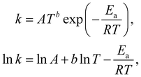 | (4) |
where A is the prefactor, T is the temperature, b is the fitting parameter for temperature dependence, Ea is the activation energy, and R is the gas constant. Eqn (2)–(4) can be integrated as an NN architecture, as shown in Fig. 1a. The inputs of the NN are the logarithm of the concentrations of species; the weights and biases are respectively the stoichiometric coefficients of the species and the Arrhenius law parameters of the reaction rate; the outputs of the NN are the production rates of the species.
 |
| | Fig. 1 Overview of the Bayesian chemical reaction neural network (B-CRNN). (a) A single pathway CRNN corresponding to eqn (1). By explicitly embedding the law of mass action and the Arrhenius law, the weights and biases in the CRNN have physical meanings, i.e., they are stoichiometric coefficients and the Arrhenius law parameters. (b) Illustration of the B-CRNN considering multiple pathways. In order to incorporate and quantify the uncertainty of the physical parameters and concentration trajectories, the physical parameters (NN weights) are given probabilistic distributions instead of being set as deterministic. (c) Illustration of the B-CRNN performance. The B-CRNN generates not only estimates of concentration trajectories of species (solid lines) but also the credible intervals (shaded regions). Dashed lines are the ground truth. | |
For a system with multiple reactions (four as an example), the NN pathways can be built in parallel, as shown in Fig. 1b. The production rates of the species will simply be the summation of the production rates from individual reaction pathways. The computation procedure for multiple reactions can be summarized as
| |  | (5) |
where

is the stoichiometric coefficient matrix.
Ns is the number of species,
Nr is the number of reactions. A negative element in
W indicates a reactant in the corresponding reaction. Denoting the vector concatenating the concentration of species at time
t as
Y(
t), then the CRNN (
eqn (5)) provides an estimation of the production rates
Ẏ(
t)
By integrating
eqn (6) from an initial conditions
Y0 with an appropriate ordinary differential equation solver, we can generate an estimated trajectory for the concentration of the species,
e.g. at a series of time instances,
Ŷk, (
k = 1,2,3,…,
N). With the correct stoichiometric coefficients and Arrhenius parameters, the estimated trajectory
Ŷk, (
k = 1,2,3,…,
N) should be close to the measured trajectory
Yk, (
k = 1,2,3,…,
N). Following this, the loss function for optimization of the stoichiometric coefficients and Arrhenius parameters is taken to be the difference between the measured and estimated trajectories.
From the deep learning perspective, the CRNN is hard-encoding physical laws, the law of mass action and the Arrhenius law, into the more general formulation of Neural Ordinary Differential Equation (NODE).29 By doing this, we improve (1) the interpretability of the NN since the weights and biases have clear physical meanings and (2) the generalizability of the NN. When a trained CRNN is performed on unseen data, especially out-of-distribution data, the prediction is bound by the widely-applicable physical laws instead of being generated by an arbitrarily fitted function.
2.2 Uncertainty quantification
The CRNN is originally proposed for deterministic construction of chemical kinetic models.20,21 In this paper, we assume probabilistic distributions on the weights and biases of the NN, so that the CRNN provides not only point estimates of those parameters but also their uncertainty quantification.
We denote the optimizable parameters of the CRNN as θ and look for the posterior distribution of θ, given certain measurements and estimated noise on the measurements. Based on Bayes' theorem, the posterior distribution of θ can be expressed as
| |  | (7) |
where

is the training dataset. The likelihood function is (normalized) Gaussian distribution with the following form
| |  | (8) |
where
τ·max
Yi is a normalizer and
τ is an estimation of the noise level,
e.g. 5% (
τ = 0.05). Due to the high dimensionality of
θ and nonlinearity of

with respect to
θ,
eqn (7) is generally intractable. So below we introduce two methods to sample the posterior distribution of
θ (
Fig. 2).
 |
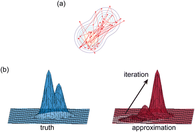
| | Fig. 2 Illustration of two Bayesian methods. (a) Hamiltonian Monte Carlo (HMC). The HMC method generates samples of B-CRNN weights by sequentially exploring the posterior distribution of the weights. (b) The variational inference method (VI). The VI method approximates the posterior distribution of the weights with a proxy distribution (normally Gaussian), by iteratively minimizing the Kullback–Leibler divergence between the proxy distribution and the true posterior distribution. | |
2.2.1 Hamiltonian Monte Carlo.
The Hamiltonian Monte Carlo (HMC) method, as a specific variant of Markov chain Monte Carlo (MCMC) algorithms, tries to approximate the posterior distribution of θ by constructing a Markov chain. The samples from the Markov chain are used to perform statistical analysis of the supposedly matched probabilistic distribution. The HMC method is proposed to suppress random walking behaviors seen in the earlier variants of MCMC30 and thus sample more efficiently in a high-dimensional space. In the HMC method, the sampling of unknown variables is equivalent to calculating the position of a particle, with the posterior distribution of the unknown variable as the potential energy of the particle. The state of a particle is sampled according to| |  | (9) |
where m is the momentum of the particle, and θ serves as the position of the particle. m is randomly initialized with  . Leapfrog steps,30L steps with stepsize ε, are taken to update the particle state.
| | 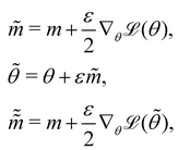 | (10) |
where ![[q with combining tilde]](https://www.rsc.org/images/entities/i_char_0071_0303.gif) and
and  are the new particle position and momentum after the update step. These new values are accepted with a probability α
| | 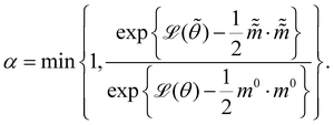 | (11) |
By repeating the above process, we can generate a sequence of samples for θ for later statistical analysis. L and ε are two adjustable parameters for HMC. They are usually automatically tuned in open source packages,31,32 such as TyXe32 used in this paper.
2.2.2 Variational inference.
Rather than sampling a Markov chain, the variational inference (VI) approach tries to approximate the true posterior distribution of θ,  , with another parameterized probabilistic distribution (usually Gaussian) q(θ|Θ) that is much easier to sample. The goal is to minimize the Kullback–Leibler (KL) divergence between q(θ|Θ) and
  , with Θ as the optimization parameters. The optimal Θ is
| |  | (12a) |
| |  | (12b) |
| |  | (12c) |
| |  | (12d) |
| |  | (12e) |
The first term of eqn (12e) is a regularization term, preventing the approximation distribution q(θ|Θ) from being totally dissimilar to the prior distribution of q. The second term of eqn (12e) is the data reconstruction term. The negation of the cost function of eqn (12e)| |  | (13) |
is often referred as the Evidence Lower Bound (ELBO),33 since it serves as the lower bound for the marginalized data probability  . The advantage of the VI approach, as will be shown in later sections, is that the optimization process is extremely fast. As for the B-CRNN, the posterior distribution of each stoichiometric coefficient/reaction constant/kinetic parameter is assumed to be individually Gaussian. Θ thus contains the means and variances of the Gaussian distributions. Mean field approximation34,35 is applied here, i.e., the Gaussian distributions of the parameters are independent to one another. Bayes by Backprop34 (BBB) is used to optimize Θ
| |  | (14a) |
| | ![[small theta, Greek, tilde]](https://www.rsc.org/images/entities/i_char_e123.gif) ∼ q(θ|Θ). ∼ q(θ|Θ). | (14b) |
Eqn (14a) is a one-sample approximation to eqn (12e). Thus, BBB can be seen as a stochastic gradient descent optimization of the VI problem in eqn (12a). After optimization, samples of θ can be easily generated from| | ![[small theta, Greek, tilde]](https://www.rsc.org/images/entities/i_char_e123.gif) ∼ q(θ|Θ*), ∼ q(θ|Θ*), | (15) |
since the distribution is Gaussian. Further statistical analysis can be performed based on these samples.
3 Application cases
3.1 An elementary reaction network without temperature dependence
The reaction system36 in this section contains 5 chemical species A, B, C, D, and E, and is described in eqn (16). 20 synthetic experiments with initial conditions randomly sampled between [0.2, 0.2, 0, 0, 0] and [1.2, 1.2, 0, 0, 0] are used for identification and uncertainty quantification of the kinetic model. The time marching step size is 0.4 s and 200 steps are simulated for each case. 5% Gaussian noise is added to the simulated concentration trajectories.| | 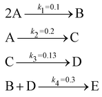 | (16) |
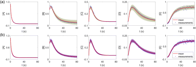
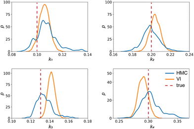
The results are shown in Fig. 3 and 4. Fig. 3(a) and (b) show the predicted uncertainty interval of concentration trajectories for all 5 species by HMC and VI methods, respectively. The results are qualitatively similar and cross-validate each other. In Fig. 4, the VI captures the modes of the HMC distribution but differences are indeed observed. This is caused by the mean field approximation35 and advanced variants of the VI method37 will likely improve the accuracy. A major difference between VI and HMC lies in the sampling speed. The HMC sampling is sequential and thus cannot leverage parallel computing for sampling acceleration. The VI sampling, after learning the parameters of the weight distribution, is equivalent to generating new samples from Gaussian distributions and is thus significantly faster than the HMC method. As an example, the sampling times for VI and HMC in this case were 489 s (500 epochs of training) + 2 s (2000 samples) = 491 s (total), and 233 s (500 samples burn-in) + 859 s (2000 samples) = 1092 s (total), respectively. This gap in the sampling speed will become more and more severe as the model size and the number of samples increase. In fact, to achieve a converged distribution, 20![[thin space (1/6-em)]](https://www.rsc.org/images/entities/char_2009.gif) 000 samples are needed (for Fig. 4, see Appendix). For this reason, in the following examples, we stick to the VI method.
000 samples are needed (for Fig. 4, see Appendix). For this reason, in the following examples, we stick to the VI method.
 |
| | Fig. 3 The (a) VI and (b) HMC results for the five species in the elementary reaction system. Blue dots are the synthetic measurements with 5% of Gaussian noise. The shaded regions indicate 4 standard deviation intervals. Red lines are the mean values of the generated trajectories. | |
 |
| | Fig. 4 The kernal density estimates of the distributions of the reaction constants for the 4 reactions in the elementary reaction system. The difference between HMC and VI results comes from the mean field approximation of the VI method. | |
Fig. 4 shows the uncertainty quantification of the rate constants from the VI method. The identified mean is close to the ground truth (except k3) and uncertain intervals for each of the constants are given.
3.2 Biodiesel production with temperature dependence and missing species
In this section, we show that the B-CRNN can handle temperature-dependent reaction systems. The reaction system38 produces biodiesel by transesterification of large, branched triglyceride (TG) molecules into methyl ester molecules. The reactions of the system38 are described as| |  | (17a) |
| |  | (17b) |
| |  | (17c) |
where DG, MG, and GL represent diglyceride, monoglyceride, and glycerol, respectively. To prepare the training dataset, 30 experiments were simulated with initial conditions randomly sampled between [0.2, 0.2, 0, 0, 0, 0] and [2.2, 2.2, 0, 0, 0, 0], and the temperature was randomly drawn from [323, 343] K. In this case, the reaction rates are represented by the Arrhenius law, with the Arrhenius parameters ln![[thin space (1/6-em)]](https://www.rsc.org/images/entities/char_2009.gif) A = [18.60,19.13,7.93] and Ea = [14.54,14.42,6.47] kcal mol−1.
A = [18.60,19.13,7.93] and Ea = [14.54,14.42,6.47] kcal mol−1.
First, we study the scenario where the information is complete, i.e., the concentration trajectories of all species are known. The VI uncertainty quantification results under different measurement noise levels are shown in Fig. 5. Fig. 5(a) contains the uncertainty intervals for the concentration trajectories of TG and DG with 1%, 5%, and 9% Gaussian noise. As the noise level increases, the uncertainty intervals also increase, as expected. Fig. 5(b) and (c) show the calculated distribution of the stoichiometric parameter of TG and the logarithm of activation energy of the reaction eqn (17a). As the noise level increases, these distributions also become more spread.
 |
| | Fig. 5 (a) The uncertainty intervals for TG and DG under Gaussian noise level 1%, 5%, and 9% (from left to right) at the same initial conditions. Blue dots are noisy measurements. (b) The calculated distribution of the stoichiometric parameter of TG in eqn (17a) (W11 stands for the element in row 1 and column 1 in W). Red dashed line indicates the true value. (c) The calculated distribution of the activation energy of eqn (17a). Red dashed line indicates the true value. The initial conditions for the shown case are [1.98, 1.93, 0, 0, 0, 0]. | |
The VI uncertainty quantification results in the scenario with a missing species are shown in Fig. 6. In this scenario, we assumed that the concentration measurements of the intermediate species DG was completely missing.20 Physically, the stoichiometric coefficients of intermediate species should not be all positive nor negative. Therefore, such constraints were implemented during the training of CRNN. The results in Fig. 6 show that the B-CRNN can still provide high-quality uncertainty estimations when the intermediate species is missing. However, since the constraint on the weight/solution space is lesser due to missing information, we observe enlarged uncertainty intervals compared with when the information is complete. This is more pronounced for the missing species DG.
 |
| | Fig. 6 Influence of missing species profiles of DG on the predictions and uncertainties. Blue dots are the synthetic measurements with 5% of Gaussian noise. Red and green curves are predictions by the B-CRNN model trained with all species profiles and with all species but missing DG profiles, respectively. The two solid lines with the same color indicate the uncertainty intervals of 4 standard deviations, while the dashed lines are the corresponding mean predictions. When the information on DG is missing for the training, the B-CRNN can still infer the chemical model but with an increased level of uncertainty, especially for TG and DG. The initial conditions for the shown case are [1.98, 1.93, 0, 0, 0, 0]. | |
3.3 Reversible reaction: enzyme–substrate reaction
In this section, we show how the B-CRNN accounts for reversible reactions. The case considered here is the Michaelis–Menten kinetic model for enzyme kinetics, described by the following equation| |  | (18) |
where E, S, ES, and P represent enzyme, substrate, enzyme–substrate complex, and product, respectively. The enzyme–substrate binding is reversible, with forward reaction rate kf and reverse reaction rate kr. The product formation is irreversible with reaction rate kcat. Since the forward and reverse directions of a reversible reaction have exactly opposite stoichiometric coefficients, such physical constraint is imposed on the stoichiometry matrix W as| |  | (19) |
where Wa is the actual weight matrix to be determined. The computation procedure is the same as eqn (5).
A total of 30 cases with 5% Gaussian noise were generated. The initial conditions of E and S were randomly generated from [1, 9], and [2, 10] respectively. The reaction rate constants are kf = 2.5, kr = 1.0, and kcat = 1.5. We further assumed at most 2 reversible reactions and 4 species, i.e.,  . The uncertainty quantification results are shown in Fig. 7(a). The identification results can be extracted as two reactions
| |  | (20) |
which is mathematically equivalent to the ground truth reaction mechanism. We further demonstrate the necessity of embedding the physical constraint with the technique shown in
eqn (19) with a hypothetical reversible reaction only considering the left half of
eqn (18)
. The results of CRNN with and without considering
eqn (19) are compared in
Fig. 7(b). With the physics embedded, the CRNN is able to reconstruct the reaction mechanism accurately while otherwise cannot.
 |
| | Fig. 7 (a) The predictions and uncertainty quantification of the reversible enzyme–substrate reactions. The shaded regions indicate 4 standard deviations. (b) The comparison between CRNN with (solid lines) and without (dashed lines) considering eqn (19) when model a hypothetical reversible reaction  . Dots indicate the synthetic measurements with 5% of Gaussian noise. The initial conditions for the shown cases are [6.46, 7.57, 0, 0] (a) and [1.78, 4.68, 0] (b). . Dots indicate the synthetic measurements with 5% of Gaussian noise. The initial conditions for the shown cases are [6.46, 7.57, 0, 0] (a) and [1.78, 4.68, 0] (b). | |
3.4 Catalytic reaction
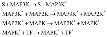
In this section, we demonstrate the B-CRNN on catalytic reactions with a weight decoupling modification. The reaction system considered in this section is the mitogen activated protein kinases (MAPK) pathway.39 Mathematically, the MAPK pathway is modeled using the following reaction rate equations.
Activation
De-activation
| | 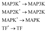 | (21) |
The reactions can be categorized into activation/phosphorylation reactions and de-activation/dephosphorylation reactions. S represents the initial stimulus, TF is the transcription factor. MAPK, MAP2K, and MAP3K represent the 3 stages of kinases. To prepare the training dataset, a total of 70 experiments were simulated with the initial conditions of all species randomly sampled within [0.1, 1] and with 5% Gaussian noise subsequently added.
In this case, several species act as catalysts in different reactions. The reaction of these catalysts do not strictly follow the form in eqn (5) (to be exact opposite between Win and Wout), since the catalysts affect the reaction rates but are not consumed. Consequently, we introduced a channel selection weight matrix Wc, the elements of which are either 0 or 1.
| |  | (22) |
where·indicates element-wise multiplication. In practice, the elements were constrained in the region [0,1] during training. The non-zero elements were normalized to 1 after training with the reaction rate constants
k normalized accordingly. The B-CRNN imported the results from the deterministic CRNN and fixed the channel selection matrix
Wc. Gaussian distribution is only assumed on
W and
k. The B-CRNN results are illustrated in
Fig. 8. The concentration of S remains almost constant and unity with a narrow uncertainty range, since S is a pure catalyst. Other species have varying concentration trajectories and uncertainties since they simultaneously serve as reactants/products and catalysts.
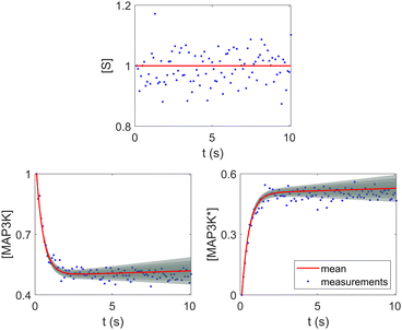 |
| | Fig. 8 Selected species profiles for the catalyst reaction case. The shaded regions indicate 4 standard deviations. | |
4 Discussion
4.1 The importance of embedding physical laws
In this section, we demonstrate the importance of incorporating physical knowledge into neural networks, from the perspective of uncertainty quantification. We compared the UQ performance of the CRNN with that of a multilayer perceptron (MLP) integrated under NODE. The MLP has one hidden layer and 100 neurons per layer. The activation function is ReLU. We first trained a deterministic MLP on the elementary reaction system in Section 3.1, which can fit the measured concentration trajectories perfectly, then used the trained MLP as an initialization for the subsequent uncertainty quantification via VI. The training dataset is the same for the CRNN and the MLP. The results from MLP and CRNN are compared in Fig. 9. It is observed that the uncertainty intervals of MLP are in general larger than those of CRNN. Also, the mean trajectories of MLP sometimes deviate from the measured trajectories (and the ground truth trajectories). Since VI effectively introduces regularization for the optimization objective as eqn (14a), the estimation could be biased. Compared to the MLP, the CRNN reduces the number of weights needed to fit the data by taking a domain-specific functional form inspired by physical laws, so the potential bias is reduced.
 |
| | Fig. 9 Uncertainty quantification comparisons between the CRNN and an MLP (without physical laws embedded). Measurements contain 5% Gaussian noise. | |
It is worth mentioning that there are literature40–42 on the more general topic of Bayesian NODE (similar to the MLP case shown above). However, B-CRNN is still valuable since it is dedicated to the modeling of chemical reaction systems with domain-specific physical laws embedded, eventually leading to better interpretability and tighter uncertainty bounds.
4.2 Incomplete information
The CRNN and its Bayesian uncertainty quantification can also accommodate a moderate amount of incomplete information. This is partially validated in Section 3.2, where the information on an intermediate species is missing. In this section, we demonstrate the applicability of the B-CRNN to scenarios where a temporal segment of concentration measurements for all species is missing. We again utilized the reaction system in Section 3.1. The meta settings remain the same, such as the measurement time interval, the noise level, the CRNN structure, and so on. The results are shown in Fig. 10. We assumed no measurements in the time interval [2, 28] s, corresponding to almost a third of the information missing in the entire 80 s reaction time span. Moreover, the segment of missing information contains the “peak concentration” parts for species C and D, which should be the most informative parts for reaction dynamics. Interestingly, B-CRNN can still infer the chemical model from data and perform uncertainty quantification, which further validates the robustness of the method.
 |
| | Fig. 10 The B-CRNN results on the same case as shown in Fig. 3, but with missing measurements in the [2, 28] s time span. The shaded regions indicate 4 standard deviations. | |
4.3 Model mixing
In practice, the exact number of reactions may not be known a priori, inevitably influencing the uncertainty quantification of CRNN. This is pronounced when the amount of available experimental data is small (5 noisy experiments in this section). Consequently, there might be multiple models that can provide reasonably good agreement with the experiments. The B-CRNN framework can provide an overall uncertainty estimation considering all inferred models.
Suppose that we have a collection of possible models  . The predictive posterior distribution of the concentration trajectory ỹ, given an unseen initial condition
 ![[x with combining tilde]](https://www.rsc.org/images/entities/b_char_0078_0303.gif) , is
, is
| |  | (23) |
where
![[small theta, Greek, tilde]](https://www.rsc.org/images/entities/i_char_e123.gif) ij
ij is the
ith sample of the model parameters from the
jth model. The prior distribution of

can be set as a truncated Poisson distribution
43 with
meta-parameter
λ| |  | (24) |
In practice, we calculate the mean trajectory prediction and standard deviations as the weighted sum of the corresponding values from all viable models, with the weights from
eqn (24). For the biodiesel case in Section 3.2, the parameters are set as
Nj = 3,
k1,
k2,
k3 = 3, 4, 5, respectively, and
λ = 3. The minimum value of
k is set as 3 because with
k = 2 the CRNN is unable to fit the data accurately enough.
20 The value for
λ is set so that the mode of the prior distribution is the same as the minimum
k. The predictive posterior distribution is illustrated in
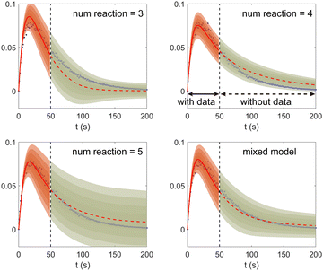
Fig. 11. The training dataset contains 5 experiments with 5% Gaussian noise and 1 s measurement time interval. Only the measurements within [0, 50] s are used for training. Those within [50, 200] s were not used in training and only displayed here for evaluation of the long-term uncertainty prediction of the B-CRNN. With different numbers of reactions assumed, the uncertainty regions can be significantly different. The model mixing, by considering different types of variations from different assumptions on the number of reactions, provides a more reasonable uncertainty interval estimation especially in the long-term prediction, as shown in the last subfigure.
 |
| | Fig. 11 The uncertainty quantification results (a–c) for three viable CRNN models assuming different numbers of reactions, and (d) for the mixed model considering all three models. Shaded regions indicate 4 standard deviations for each model. Only data within [0, 50] s were used to train the models. Data within [50, 200] s is shown for performance comparison. | |
4.4 Uncertainty quantification on selected parameters
When the molecular formulas of reactants and products are known, the conservation of elements can be used to establish the stoichiometric parameters. In this scenario, UQ is only necessary on the kinetic parameters. It is quite straightforward to perform UQ only on selected parameters. One only needs to assume Gaussian distributions on the uncertain parameters and use deterministic values for the certain ones. In Fig. 12, we show the comparison between UQ on all parameters and UQ on kinetic parameters only for the biodiesel system in Section 3.2. The measurement data and optimization hyperparameter settings are all kept the same. Since the UQ on kinetic parameters only involve 6 uncertain parameters, the uncertain intervals for some species such as TG, GL, and R'CO2R are smaller than those of UQ on all parameters involves 24 uncertain parameters.
 |
| | Fig. 12 Comparison between UQ on all parameters and UQ on kinetic parameters only for the biodiesel system. The initial conditions are the same as Fig. 6. Blue dots are the synthetic measurements with 5% of Gaussian noise. Red and green curves mark the uncertain intervals (4 standard deviations) by the B-CRNN model performing UQ on all parameters and kinetic parameters, respectively. The dashed lines are the corresponding mean predictions. When performing UQ on kinetic parameters only, since the number of uncertain variables decreases significantly (from 24 to 6 in this case), the uncertainty intervals become tighter. | |
5 Conclusions
In this paper, we have proposed the Bayesian chemical reaction neural network (B-CRNN), a probabilistic version of the original deterministic CRNN. The Bayesian CRNN is able to simultaneously infer the chemical reaction pathways from measured noisy concentration data and perform uncertainty quantification on the identified reaction pathways, kinetic parameters, and concentration predictions with unseen initial conditions. Two methods were proposed and introduced in detail to implement the Bayesian CRNN: Hamiltonian Monte Carlo and variational inference. Their results are shown to be qualitatively similar, but variational inference was adopted for further demonstrations due to its speed and interpretability. We validated the Bayesian CRNN on four chemical systems, showing that with necessary modifications the Bayesian CRNN is able to deal with the temperature dependence of reaction rates, incomplete information with missing intermediate species, reversible reactions, and catalytic reactions. We further discussed three issues: (1) The importance of embedding physical laws in CRNN was demonstrated by using an MLP integrated by NODE to fit the same data. The MLP provided a larger uncertainty estimation for its variation flexibility is larger than that of the CRNN. (2) The Bayesian CRNN can be applied to scenarios where a significant portion of information in time is missing. (3) When the amount of available data is limited, there could be multiple viable models fitting the data reasonably well. Integrating Bayesian CRNN with model mixing can consider all viable models and provide prediction with uncertainty for unseen scenarios.
Generally speaking, there is no theoretical hurdles preventing the B-CRNN from application on larger-scale more complex chemical systems across disciplines, such as combustion and biochemical systems. One of the potential issues is that training CRNN could be difficult because of the stiffness issue commonly encountered in combustion systems. Another issue is that the amount of data needed grows as the considered system grows larger, which may reduce the training speed and raise the question of data availability (e.g. in biochemical systems). The former could be solved by incorporating more advanced neural network training schemes.44,45 The latter may require integrating B-CRNN with active learning for efficient experimental design. Nonetheless, the B-CRNN framework opens new opportunities to applying physics-informed machine learning techniques in chemical systems for model inference and uncertainty quantification.
Author contributions
Qiaofeng Li: Methodology, investigation, writing – original draft. Huaibo Chen: investigation, writing – original draft. Benjamin C. Koenig: methodology, writing – review and editing. Sili Deng: conceptualization, funding acquisition, writing – review and editing.
Conflicts of interest
There are no conflicts to declare.
Appendices
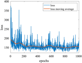
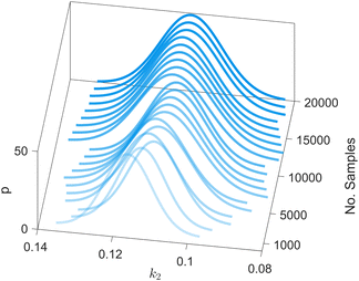
We provide additional information to show that the HMC sampling and VI training have converged with the provided settings in Section 3.1. The fitted normal density functions with the HMC samples are shown in Fig. 13. As more samples are included, eventually to 20![[thin space (1/6-em)]](https://www.rsc.org/images/entities/char_2009.gif) 000 samples, the fitted functions gradually converge. The VI training loss history is shown in Fig. 14. The blue loss history shows large oscillation because in each epoch a random sample is drawn from the posterior distribution of parameters to calculate the loss. The moving average loss history is averaged over adjacent 1000 samples. The training is converged after 1000 epochs based on the moving average loss.
000 samples, the fitted functions gradually converge. The VI training loss history is shown in Fig. 14. The blue loss history shows large oscillation because in each epoch a random sample is drawn from the posterior distribution of parameters to calculate the loss. The moving average loss history is averaged over adjacent 1000 samples. The training is converged after 1000 epochs based on the moving average loss.
 |
| | Fig. 13 The fitted normal density functions based on different numbers of samples using HMC. | |
 |
| | Fig. 14 The training loss history and the moving average (over 100 adjacent data points) of the VI for the case in Section 3.1. | |
Acknowledgements
The work is supported by National Science Foundation under Grant No. CBET-2143625. QL would like to thank Dr Weiqi Ji and Suyong Kim for their assistance in validating the results. HC would like to thank Dr Qinghui Meng at Columbia University for the helpful discussion. BCK is partially supported by the National Science Foundation Graduate Research Fellowship under Grant No. 1745302.
References
- A. Y. Poludnenko, J. Chambers, K. Ahmed, V. N. Gamezo and B. D. Taylor, Science, 2019, 366, eaau7365 CrossRef CAS PubMed.
- L. Yin, Y. Jia, X. Guo, D. Chen and Z. Jin, Int. J. Heat Mass Transfer, 2019, 133, 129–136 CrossRef CAS.
- B. Sanchez, J.-L. Santiago, A. Martilli, M. Palacios and F. Kirchner, Atmos. Chem. Phys., 2016, 16, 12143–12157 CrossRef CAS.
-
Y. Shi, H.-W. Ge and R. D. Reitz, Computational optimization of internal combustion engines, Springer Science & Business Media, 2011 Search PubMed.
- C. W. Gao, J. W. Allen, W. H. Green and R. H. West, Comput. Phys. Commun., 2016, 203, 212–225 CrossRef CAS.
- T. Lu and C. K. Law, Prog. Energy Combust. Sci., 2009, 35, 192–215 CrossRef CAS.
- M. Aldén, Proc. Combust. Institute, 2022 DOI:10.1016/j.proci.2022.06.020.
- M. Schmidt and H. Lipson, Science, 2009, 324, 81–85 CrossRef CAS PubMed.
- S. H. Rudy, S. L. Brunton, J. L. Proctor and J. N. Kutz, Sci. Adv., 2017, 3, e1602614 CrossRef PubMed.
- K. Champion, B. Lusch, J. N. Kutz and S. L. Brunton, Proc. Natl. Acad. Sci. U. S. A., 2019, 116, 22445–22451 CrossRef CAS PubMed.
- M. Frenklach, A. Packard, P. Seiler and R. Feeley, Int. J. Chem. Kinet., 2004, 36, 57–66 CrossRef CAS.
- D. A. Sheen and H. Wang, Combust. Flame, 2011, 158, 2358–2374 CrossRef CAS.
- T. Turányi, T. Nagy, I. G. Zsély, M. Cserháti, T. Varga, B. T. Szabó, I. Sedyo, P. T. Kiss, A. Zempleni and H. J. Curran, Int. J. Chem. Kinet., 2012, 44, 284–302 CrossRef.
- K. Braman, T. A. Oliver and V. Raman, Combust. Theory Modelling, 2013, 17, 858–887 CrossRef CAS.
- N. M. Mangan, S. L. Brunton, J. L. Proctor and J. N. Kutz, IEEE Trans. Mol., Biol. Multi-Scale Commun., 2016, 2, 52–63 Search PubMed.
- M. Hoffmann, C. Fröhner and F. Noé, J. Chem. Phys., 2019, 150, 025101 CrossRef PubMed.
- W. E, Communications in Computational Physics, 2020, 28(5), 1639–1670 CrossRef.
-
J. Devlin, M.-W. Chang, K. Lee and K. Toutanova, arXiv, 2018, arXiv:1810.04805 DOI:10.48550/arXiv.1810.04805.
- R. Ranade, S. Alqahtani, A. Farooq and T. Echekki, Fuel, 2019, 251, 276–284 CrossRef CAS.
- W. Ji and S. Deng, J. Phys. Chem. A, 2021, 125, 1082–1092 CrossRef CAS PubMed.
- W. Ji, F. Richter, M. J. Gollner and S. Deng, Combust. Flame, 2022, 240, 111992 CrossRef CAS.
- H. Wang and D. A. Sheen, Prog. Energy Combust. Sci., 2015, 47, 1–31 CrossRef.
- J. Wang, Z. Zhou, K. Lin, C. K. Law and B. Yang, Combust. Flame, 2020, 213, 87–97 CrossRef CAS.
- J. A. Miller, R. Sivaramakrishnan, Y. Tao, C. F. Goldsmith, M. P. Burke, A. W. Jasper, N. Hansen, N. J. Labbe, P. Glarborg and J. Zádor, Prog. Energy Combust. Sci., 2021, 83, 100886 CrossRef.
- J. Badra, A. Elwardany and A. Farooq, Proc. Combust. Institute, 2015, 35, 189–196 CrossRef CAS.
- M. Frenklach, Proc. Combust. Institute, 2007, 31, 125–140 CrossRef.
- W. Ji, J. Wang, O. Zahm, Y. M. Marzouk, B. Yang, Z. Ren and C. K. Law, Combust. Flame, 2018, 190, 146–157 CrossRef CAS.
- W. Ji, Z. Ren, Y. Marzouk and C. K. Law, Proc. Combust. Institute, 2019, 37, 2175–2182 CrossRef CAS.
-
R. T. Chen, Y. Rubanova, J. Bettencourt and D. K. Duvenaud, Adv. Neural Information Processing Systems, arXiv, 2018, 31, arXiv:1806.07366 DOI:10.48550/arXiv.1806.07366.
-
S. Brooks, A. Gelman, G. Jones and X.-L. Meng, Handbook of Markov chain Monte Carlo, CRC press, 2011 Search PubMed.
- E. Bingham, J. P. Chen, M. Jankowiak, F. Obermeyer, N. Pradhan, T. Karaletsos, R. Singh, P. A. Szerlip, P. Horsfall and N. D. Goodman, J. Mach. Learn. Res., 2019, 20, 28:1–28:6 Search PubMed.
- H. Ritter and T. Karaletsos, Proc. Machine Learn. Syst., 2022, 398–413 Search PubMed.
-
D. P. Kingma and M. Welling, arXiv, 2013, arXiv:1312.6114 DOI:10.48550/arXiv.1312.6114.
-
C. Blundell, J. Cornebise, K. Kavukcuoglu and D. Wierstra, International conference on machine learning, 2015, pp. 1613–1622 Search PubMed.
- L. Yang, X. Meng and G. E. Karniadakis, J. Comput. Phys., 2021, 425, 109913 CrossRef.
-
D. P. Searson, M. J. Willis and A. Wright, Reverse Engineering Chemical Reaction Networks from Time Series Data, John Wiley & Sons, Ltd, 2012, ch. 12, pp. 327–348 Search PubMed.
-
K. P. Murphy, Probabilistic Machine Learning: Advanced Topics, MIT Press, 2023 Search PubMed.
- D. Darnoko and M. Cheryan, J. Am. Oil Chem. Soc., 2000, 77, 1263–1267 CrossRef CAS.
- J. Xing, D. D. Ginty and M. E. Greenberg, Science, 1996, 273, 959–963 CrossRef CAS PubMed.
-
E. D. Brouwer, J. Simm, A. Arany and Y. Moreau, 2019, GRU-ODE-Bayes: continuous modeling of sporadically-observed time series, Proceedings of the 33rd International Conference on Neural Information Processing Systems, pp. 7379–7390.
-
R. Dandekar, V. Dixit, M. Tarek, A. Garcia-Valadez and C. Rackauckas, arXiv, 2020, arXiv:2012.07244 DOI:10.48550/arXiv.2012.07244.
- M. A. Bhouri and P. Perdikaris, Philos. Trans. R. Soc., A, 2022, 380, 20210201 CrossRef PubMed.
- G. Yan, H. Sun and H. Waisman, Comput. Struct., 2015, 152, 27–44 CrossRef.
- Z. Yao, A. Gholami, S. Shen, K. Keutzer and M. W. Mahoney, AAAI, 2021, 9, 093122 Search PubMed.
- S. Kim, W. Ji, S. Deng, Y. Ma and C. Rackauckas, Chaos, 2021, 31, 093122 CrossRef PubMed.
|
| This journal is © the Owner Societies 2023 |
Click here to see how this site uses Cookies. View our privacy policy here.  Open Access Article
 ,
Huaibo
Chen
,
Benjamin C.
Koenig
and
Sili
Deng
,
Huaibo
Chen
,
Benjamin C.
Koenig
and
Sili
Deng
 *
*


 is the stoichiometric coefficient matrix. Ns is the number of species, Nr is the number of reactions. A negative element in W indicates a reactant in the corresponding reaction. Denoting the vector concatenating the concentration of species at time t as Y(t), then the CRNN (eqn (5)) provides an estimation of the production rates Ẏ(t)
 is the training dataset. The likelihood function is (normalized) Gaussian distribution with the following form
 with respect to θ, eqn (7) is generally intractable. So below we introduce two methods to sample the posterior distribution of θ (Fig. 2).

 . Leapfrog steps,30L steps with stepsize ε, are taken to update the particle state.
![[q with combining tilde]](https://www.rsc.org/images/entities/i_char_0071_0303.gif) and
and  are the new particle position and momentum after the update step. These new values are accepted with a probability α
 , with another parameterized probabilistic distribution (usually Gaussian) q(θ|Θ) that is much easier to sample. The goal is to minimize the Kullback–Leibler (KL) divergence between q(θ|Θ) and
  , with Θ as the optimization parameters. The optimal Θ is


 . The advantage of the VI approach, as will be shown in later sections, is that the optimization process is extremely fast. As for the B-CRNN, the posterior distribution of each stoichiometric coefficient/reaction constant/kinetic parameter is assumed to be individually Gaussian. Θ thus contains the means and variances of the Gaussian distributions. Mean field approximation34,35 is applied here, i.e., the Gaussian distributions of the parameters are independent to one another. Bayes by Backprop34 (BBB) is used to optimize Θ
![[small theta, Greek, tilde]](https://www.rsc.org/images/entities/i_char_e123.gif) ∼ q(θ|Θ).
∼ q(θ|Θ).![[small theta, Greek, tilde]](https://www.rsc.org/images/entities/i_char_e123.gif) ∼ q(θ|Θ*),
∼ q(θ|Θ*),
![[thin space (1/6-em)]](https://www.rsc.org/images/entities/char_2009.gif) 000 samples are needed (for Fig. 4, see Appendix). For this reason, in the following examples, we stick to the VI method.
000 samples are needed (for Fig. 4, see Appendix). For this reason, in the following examples, we stick to the VI method.


![[thin space (1/6-em)]](https://www.rsc.org/images/entities/char_2009.gif) A = [18.60,19.13,7.93] and Ea = [14.54,14.42,6.47] kcal mol−1.
A = [18.60,19.13,7.93] and Ea = [14.54,14.42,6.47] kcal mol−1.


 . The uncertainty quantification results are shown in Fig. 7(a). The identification results can be extracted as two reactions
 . The results of CRNN with and without considering eqn (19) are compared in Fig. 7(b). With the physics embedded, the CRNN is able to reconstruct the reaction mechanism accurately while otherwise cannot.

 . Dots indicate the synthetic measurements with 5% of Gaussian noise. The initial conditions for the shown cases are [6.46, 7.57, 0, 0] (a) and [1.78, 4.68, 0] (b).


 . The predictive posterior distribution of the concentration trajectory ỹ, given an unseen initial condition
 ![[x with combining tilde]](https://www.rsc.org/images/entities/b_char_0078_0303.gif) , is
, is
![[small theta, Greek, tilde]](https://www.rsc.org/images/entities/i_char_e123.gif) ij is the ith sample of the model parameters from the jth model. The prior distribution of
ij is the ith sample of the model parameters from the jth model. The prior distribution of  can be set as a truncated Poisson distribution43 with meta-parameter λ

![[thin space (1/6-em)]](https://www.rsc.org/images/entities/char_2009.gif) 000 samples, the fitted functions gradually converge. The VI training loss history is shown in Fig. 14. The blue loss history shows large oscillation because in each epoch a random sample is drawn from the posterior distribution of parameters to calculate the loss. The moving average loss history is averaged over adjacent 1000 samples. The training is converged after 1000 epochs based on the moving average loss.
000 samples, the fitted functions gradually converge. The VI training loss history is shown in Fig. 14. The blue loss history shows large oscillation because in each epoch a random sample is drawn from the posterior distribution of parameters to calculate the loss. The moving average loss history is averaged over adjacent 1000 samples. The training is converged after 1000 epochs based on the moving average loss.
