Revealing nanoscale slip within Taylor–Aris dispersion

Abstract

Hydrodynamic slip at fluid–solid interfaces plays an important role in a range of transport phenomena, especially in fluids under small-scale confinement. Much work has studied the microscopic origins of slip. In this work, we explore the connection between the microscopic slip velocity and the macroscopic (slip-adjusted) Taylor–Aris dispersion in the fluid, which enables the former to be written in terms of the latter. Through extensive molecular-dynamics simulations of simple and polymeric fluids under a wide range of thermodynamic and geometric conditions, we show that the continuum treatment of Taylor–Aris dispersion can be readily extended to systems where the confining length-scale is comparable to the slip length. We further demonstrate that slip velocity can be accurately inferred through measurements of equilibrium and shear-augmented molecular self-diffusivities.

---

Gerald J. Wang

Gerald “Jerry” Wang is an Assistant Professor of Civil and Environmental Engineering, and Chemical Engineering (by courtesy) and Mechanical Engineering (by courtesy), at Carnegie Mellon University. He received his BS from Yale University (Mechanical Engineering, Mathematics and Physics), SM from MIT (Mechanical Engineering), and PhD from MIT (Mechanical Engineering and Computation). He was a postdoctoral researcher at MIT in Chemical Engineering and is an EIT in Electrical and Computer Engineering. At CMU, Jerry directs the M5 Lab, which focuses on computational small-scale mechanics of fluids, soft matter, and active matter, with applications across energy, food, sustainable materials, and urban livability.

---

1 Introduction

The continuum treatment of fluids frequently presumes zero hydrodynamic slip at a fluid–solid interface (the no-slip boundary condition). However, non-zero slip at fluid–solid interfaces can play an important role in transport phenomena at interfaces^1,2 and under confinement, especially in systems where a confining length-scale is comparable to the slip length.³

Owing to the fact that slip is intrinsically a microscopic phenomenon, a significant body of work using both experiments and molecular-dynamics (MD) simulations has sought to characterize the microscopic mechanisms underlying slip, as reviewed in previous work.^4,5 Many studies have investigated the microscopic kinetics of slip within the broad (and interrelated) frameworks of thermally activated rate processes,^6,7 molecular-kinetic theory,^8–11 and biased Brownian motion.¹² Slip has been studied in relation to microscopic friction at the fluid–solid interface^13–16 and also as a function of microscopic roughness and surface texture.^17,18 All of the aforementioned work focuses on relating the slip phenomenon with microscopic aspects of the system, with no explicit connection to macroscopic fluid mechanics.

In contrast, a distinct body of work on slip explores its connections with continuum-scale descriptions of a fluid. Several studies have explored slip within the framework of continuum fluid mechanics; these studies infuse microscopic details into a fundamentally macroscopic picture via, e.g., a corrugated potential energy landscape representative of the boundary.^19,20 Hsu and Patankar²¹ demonstrated that the relationship between slip and fluid shear rate (supported both by molecular-scale simulations and experiments) can be qualitatively recovered using a continuum treatment of a compressible fluid in the presence of a wall that imposes a potential on the fluid.

The present work follows in the spirit of the latter by studying the validity of (appropriately interpreted) continuum theory in the limit of small confining length-scales. In particular, we address the following question: “Does the continuum theory of Taylor–Aris dispersion describe the relationship between shear rate and shear-enhanced diffusivity in a nanoscale channel with non-negligible hydrodynamic slip?” We answer this question in the affirmative, and show as a consequence that the classical theory can be inverted to infer details about slip using only measurements of diffusivity. The closest related work²² to that carried out here presents purely classical results (both analytical and numerical, via finite volumes) for the relationship between dispersion and slip; our focus here is on seamlessly extending the classical theory to channels of nanoscale dimension, validated using molecular simulations.

In the following section, we model slip velocity in terms of equilibrium and shear-augmented diffusivities in plane-Couette flow. We describe our numerical experiments in section 3 (and Appendix A), with results discussed in section 4, followed by concluding remarks and future directions in section 5.

2 Theory: Taylor–Aris dispersion in the presence of hydrodynamic slip at the fluid–solid interface

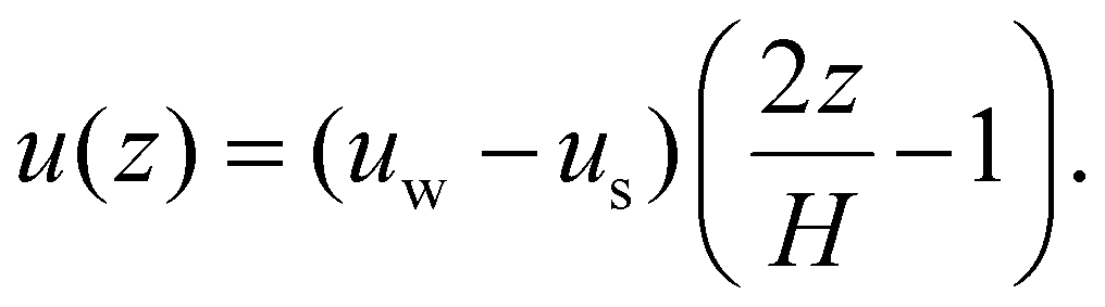
Consider the schematic for plane-Couette flow shown in Fig. 1a, with fluid sheared by two solid walls moving opposite to each other along the x-direction (the streamwise direction) with equal speeds u_w. The walls, separated by a gap height H in the z-direction (the wall-normal direction) and of infinite extent in the y-direction (the spanwise direction) and the x-direction, are identical in microstructure, yielding equal slip velocity u_s at both interfaces. The steady and fully-developed streamwise fluid velocity with slip boundary conditions is:

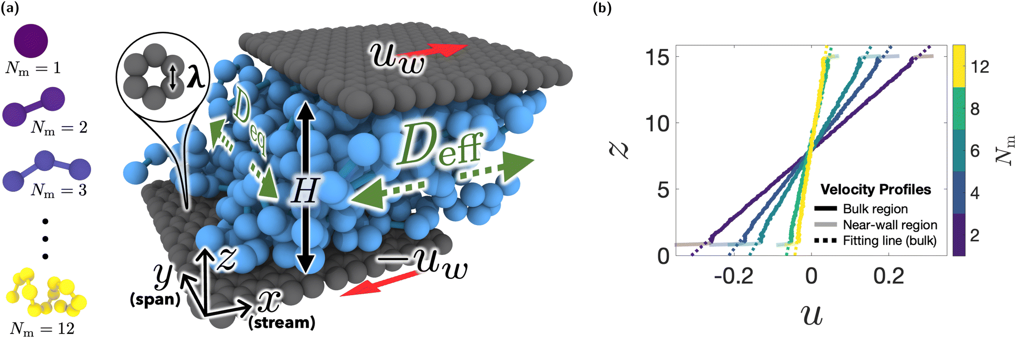Fig. 1 (a) Schematic of simulated plane-Couette flow for a fluid (LJ chains with N_m = 5) confined by two identical graphene walls with nearest-neighbor distance λ and gap height H and fluid self-diffusion coefficient in the streamwise direction D_eff and spanwise direction D_eq. Fluids with different chain lengths simulated in this study are shown on the left. (b) Steady-state fluid velocity profiles at u_w = 0.74 for LJ chains drawn from dataset 4 (Table 1). Linear fits to velocity profiles are performed in the bulk region and are extrapolated to the wall locations to calculate slip velocity. All quantities are non-dimensionalized as discussed in section 3.

Following the classic arguments by Aris and Taylor,^23,24 and assuming no slip, the ratio of the shear-augmented (effective) diffusivity D_eff to the equilibrium diffusivity D_eq (diffusivity in a non-sheared direction) is:

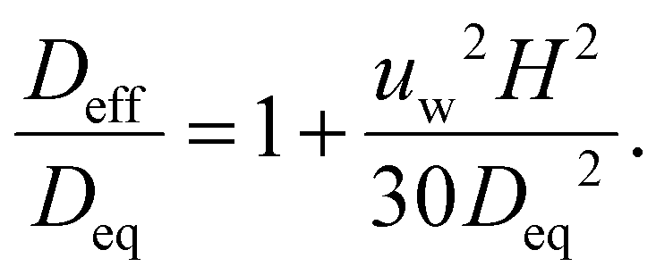
In the slip case, since the fluid velocity at the boundaries has magnitude u_w − u_s, this ratio is:

An extended discussion of eqn (2) and (3) is presented in the ESI.†

The core premise of this work is the observation that eqn (3) establishes a connection between the slip velocity and the extent to which the diffusivity is enhanced by shear. In particular, eqn (3) can be inverted to obtain slip velocity in terms of the equilibrium and shear-augmented diffusivities:

u_s = u_w − u_D, (4)

where

Here, u_D can be physically interpreted as the interfacial fluid velocity, i.e., u_D = |u(z = 0)| = |u(z = H)|. It is worth emphasizing that eqn (5) constructs a velocity-scale using only diffusivity-scales (and the length-scale H) and makes no reference to any other velocities in the system. Any approach that yields estimates of D_eq and D_eff can thus also be used to obtain an estimate of u_s. Within a plane-Couette MD simulation, estimates for both diffusion coefficients can be obtained via the Einstein–Helfand relation,^25–27 with D_eq computed from kinematics in the spanwise direction and D_eff computed from kinematics in the streamwise direction. In particular, for any collection of particles viewed in a reference frame in which they have no net center-of-mass motion, we can compute that collection's mean-squared displacement (MSD) in the Cartesian direction k as:

〈r_k²(t_sample)〉 = 〈|r_k(t_sample) − r_k(0)|²〉, (6)

where r_k is the k-direction coordinate of a particle, t_sample denotes the length of the measurement window, and the angle brackets indicate an average computed over all particles in the collection. Eqn (6) is computed in a reference frame in which the system's overall center of mass is stationary; we discuss the limits of validity for this approach to measuring diffusivity in Appendix B. From here, the Einstein–Helfand relation gives:

D_eff = 〈r_x²(t_sample)〉/(2t_sample) (7)

D_eq = 〈r_y²(t_sample)〉/(2t_sample) (8)

In practice, these diffusion coefficients are computed by collecting MSD data at numerous values of t_sample and performing least-squares regression to extract the slope from a straight-line model.

3 Molecular-dynamics simulations

To validate eqn (4) and (5), we perform non-equilibrium MD simulations of plane-Couette flow of a variety of fluids, including Lennard-Jones (LJ) monomers and LJ chains of varying length (Fig. 1a), using the Large-scale Atomic/Molecular Massively Parallel Simulator (LAMMPS).²⁸ In each simulation, interactions between non-bonded particles i and j are described by the Lennard-Jones potential:where r_ij is the distance between particles i and j. In all simulations, the same length-scale σ applies for all LJ interactions (whether fluid–fluid or fluid–solid) and the energy-scale ε is ε_ff for all fluid–fluid interactions. Values of this energy-scale for fluid–solid interactions, ε_fs, are provided in Table 1. Throughout all simulations, all monomers, whether standalone or within a chain, have identical mass m. Each simulation features a homogeneous fluid with a single value of N_m, the number of monomers in each chain, with N_m ranging from 1 (monomers only) to 12 (the longest chains studied). Further details on these MD simulations, including the specific parameters governing bonded interactions, are provided in Appendix A.

Table 1 MD datasets classified according to various thermodynamic (T, ε_fs) and geometric (H, λ) conditions. Symbols used in Fig. (2)–(4) are shown with dataset number in parentheses. Each of the nine datasets contains 1200 MD simulations, as described in section 3

Dataset	Fluid temperature, T	Gap height, H	Fluid–solid interaction energy εfs	Nearest-neighbor distance λ
★ (1)	3.31	6.35	0.600	0.451
◀ (2)	3.31	15.9	0.533	0.451
▲ (3)	3.31	15.9	0.600	0.406
● (4)	3.31	15.9	0.600	0.451
▼ (5)	3.31	15.9	0.600	0.496
▶ (6)	3.31	15.9	0.733	0.451
+ (7)	3.97	15.9	0.600	0.451
■ (8)	4.31	12.7	0.667	0.451
× (9)	4.64	12.7	0.600	0.451

---

In what follows, all quantities are non-dimensionalized against the length-scale σ, the energy-scale ε_ff, the mass-scale m, the time-scale , the density-scale m/σ³, the diffusivity-scale , and the temperature-scale k_B/ε_ff, where k_B is the Boltzmann constant. By varying thermodynamic and geometric conditions – namely, the temperature T, the fluid–solid interaction energy ε_fs, the gap height H, and the nearest-neighbor distance λ for atoms in each wall – we generate a total of 9 datasets as shown in Table 1, each containing 12 distinct fluids (1 ≤ N_m ≤ 12) and 10 wall velocities (0.04 ≤ u_w ≤ 0.74). For the purpose of increasing statistical confidence, which is especially critical for fluid transport properties under nanoscale confinement,²⁹ each of these 1080 simulations is repeated 10-fold using different initial particle velocities drawn from the appropriate Maxwell–Boltzmann distribution at the prescribed temperature, with the corresponding results averaged.

In each simulation, we obtain the steady-state fluid velocity profile u(z) by creating uniform bins of width 0.8 along the z-direction and then computing the time- and particle-averaged velocity in each bin. Several steady-state fluid velocity profiles from dataset 4 (Table 1) at a wall velocity of u_w = 0.74 are shown in Fig. 1b. Slip velocity is measured by fitting a straight line to each velocity profile in the bulk region (defined here to be 1.5 away from each wall), extrapolating the fitted line to each of the two walls, and averaging the difference between the wall velocity and the extrapolated velocity obtained at each of the two walls. For the purpose of computing each term in eqn (5), in each simulation, we also measure the MSD (at the level of individual monomers) for , for each unconfined direction, yielding MSDs in the spanwise (Fig. 2a) and streamwise (Fig. 2b) directions.

Fig. 2 (a) Characteristic MSDs in the spanwise direction (drawn from dataset 4 and averaged over all wall velocities) as a function of sampling time and polymer chain length, which are used to measure D_eq; (b) characteristic MSDs in the streamwise direction for a monomeric fluid (N_m = 1) as a function of sampling time and wall velocity, which are used to measure D_eff.

4 Results and discussion

We find that the self-diffusion coefficient in the spanwise direction D_eq is independent of the wall velocity u_w, as expected (Fig. 3a). D_eq decreases with increasing chain length (Fig. 2a) and hence also decreases with increasing viscosity μ, in a manner consistent with previous work³⁰ (Fig. 2a). On the other hand, the diffusion coefficient in the streamwise direction D_eff increases with increasing wall velocity, a direct consequence of Taylor–Aris dispersion (Fig. 3b).

Fig. 3 Viscosity and wall velocity dependence of (a) the spanwise coefficient of self-diffusion and (b) the streamwise coefficient of self-diffusion. In both cases, models of the viscosity-dependent form discussed in Sukhishvili et al.³⁰ are overlaid. Contours of constant pre-factor a are provided as a guide to the eye in (b).

We find clear evidence that the dependence of the streamwise diffusivity on the wall velocity is poorly described by the no-slip model of dispersion (eqn (2)), which would predict D_eff/D_eq to collapse to a single line, which is specifically linear in u_w²H²/(30D_eq²) (Fig. 4a). The streamwise diffusivity is however in excellent agreement with the slip-adjusted model of dispersion (eqn (3)). As evidence of this, in Fig. 4b, we show the slip velocity inferred using the equilibrium and shear-augmented diffusivities (eqn (4)) as compared to the slip velocity measured in each MD simulation through extrapolation of the velocity profile to the wall location. We find agreement within 2.3% mean absolute error, with no systematic discrepancies as a function of any of the parameters varied. These results confirm the hypothesis that the slip velocity can in fact be inferred from the streamwise-spanwise diffusivity difference via inversion of (slip-adjusted) Taylor–Aris dispersion.

Fig. 4 (a) Normalized shear-augmented coefficient of self-diffusion vs. linear term in eqn (2); (b) slip velocity inferred via Taylor–Aris dispersion eqn (4) vs. slip velocity measured by extrapolation of fluid velocity profile to boundary (dashed line of parity overlaid).

This is an intriguing result for several reasons. Despite Taylor–Aris dispersion following from a continuum description of a fluid, this theory – when applied to molecular self-diffusivities – extends seamlessly to channels of nanoscale dimension, provided that the relevant shear rates are adjusted for slip; this result follows a pattern of macroscopic fluid-mechanical phenomena that can be observed in systems of nanoscale dimension, despite the continuum laws not being obviously applicable in such systems.⁴ Moreover, this result provides a new route by which one can determine the boundary condition (slip velocity) that is consistent with the bulk flow, which makes exclusive use of measurements of fluid diffusivity.

5 Conclusions

In this work, we investigated the connection between hydrodynamic slip at a fluid–solid boundary and Taylor–Aris dispersion in a confined fluid, leading to the relationship in eqn (4) and (5), between the slip velocity, the spanwise diffusivity, and the streamwise diffusivity. We performed MD simulations of plane-Couette flow for a wide range of fluids (simple fluids and polymers of varying length) under a wide range of thermodynamic and geometric conditions, and we observed that (slip-adjusted) Taylor–Aris dispersion accurately captures shear-augmented diffusivity in fluids under small-scale confinement. We further found excellent agreement between the slip velocity inferred from dispersion (using the streamwise–spanwise diffusivity difference) and the slip velocity measured using an approach traditional in MD simulations (using the fluid velocity profile extrapolated to the boundaries).

These results motivate several natural extensions. One such extension would be to assess the accuracy of this theory for a fluid mixture (comparing against, e.g., Zhou et al.³¹) or for fluid bounded by rough or patchy walls.¹⁷ The smallest channel studied in this work still has a majority of fluid in its bulk region, in which interfacial effects – especially fluid layering^32,33 – are negligible. The question of whether the present dispersion model can be adapted to yet-smaller channels, in which surface-driven effects play a significant role in diffusion in all directions,³⁴ remains open. Fig. 4b establishes strong agreement between two distinct approaches for measuring slip velocity, at the level of means; an intriguing direction of further study would be comparison at higher moments and for the full distributions of measured slip velocities (e.g., at the level of variances in the slip velocity). Such work could have important implications for the uncertainty quantification of slip in small-scale channels within MD simulations. Finally, we note that eqn (4) is but one example of using Taylor–Aris dispersion to formulate a nanoscale hydrodynamic quantity in terms of anisotropic diffusivities. It would be especially interesting to see whether this treatment extends to other related quantities (e.g., the fluid–solid friction coefficient).

Data availability

Data for this article, including scripts to generate the MD simulations described in section 3, are available at https://github.com/M5-Lab/NanoscaleTaylorAris.

Conflicts of interest

The authors report no conflict of interest.

Appendix A: details of MD simulations

Each system consists of a homogeneous fluid with number density ρ = 0.85 (based upon number of monomers), confined by two identical graphene walls that are squares with a side length of 9.52. A cutoff radius of 3.17 was used for all simulations. Apart from the non-bonded LJ interactions in eqn (9), intra-chain interactions in polymeric fluids are governed by: (a) a harmonic potential U_bond(r) for particles directly bonded to each other and separated by a distance r, given by U_bond(r) = (k_bond/2)(r − r₀)², with bond constant k_bond = 72.0 and equilibrium bond length r₀ = 2^1/6 (same as equilibrium distance between two non-bonded fluid particles); (b) a harmonic potential for two consecutive bonds forming an angle θ, given by U_angle(θ) = (k_angle/2)(θ − θ₀)², with angle constant k_angle = 66.7 and equilibrium bond angle θ₀ = 110°; and (c) CHARMM-style dihedral interactions³⁵ for sets of four contiguously bonded particles in the same chain with dihedral angle ϕ, given by U_dihedral(ϕ) = k_dh(1 + cos(ϕ + α_dh)), with dihedral coefficients k_dh = -18.67 and α_dh = 7°. The structures of different fluids and solids were generated using the software Moltemplate³⁶ and visualizations were rendered using the Open Visualization Tool (OVITO).³⁷ To counter the effects of viscous heating due to shear, the temperature of the fluid was maintained via a Nosé–Hoover (NH) thermostat;^38,39 we verified that the core Taylor–Aris dispersion result (Fig. 4b) is unaffected by choice of thermostat or choice of thermostat damping timescale (see ESI†). We measure viscosity of the fluid using , where τ_xz is the magnitude of the shear stress imposed by the walls on the fluid in the streamwise direction and is the fluid shear rate. τ_xz is obtained by evaluating the time-average of the difference of forces applied by the top and bottom walls on the fluid in the streamwise direction, normalized by the wall area.

Appendix B: limits of validity for system-center-of-mass-corrected diffusivity

For the purpose of evaluating eqn (6), mean-squared displacements are computed in a single reference frame with no net center-of-mass motion. In an MD simulation, this reference frame can be established by computing the average velocity for all particles in the system. For a plane-Couette flow (with the origin of velocity at the channel midline, as shown in Fig. 1a), this frame should simply be the laboratory frame, by symmetry.

It is worth emphasizing that there are limits of validity to choosing a single reference frame. In particular, this choice is only justified if particles are tracked over a sampling time sufficiently long that all particles may sample velocities throughout the channel , a critical assumption of the Taylor–Aris theory. On this timescale, for a plane-Couette flow, each individual particle has an expected velocity of the channel midline velocity, i.e., the velocity of the single reference frame described above.

Since any fluid particle not at the channel midline locally has a non-zero expected velocity (given by eqn (1)), it is important to note that when , many individual particles will have only sampled a subset of velocities. If the MSD of these particles is tracked with the single choice of reference frame described above, then this MSD will grow quadratically with time, as would be expected for ballistic transport; indeed, a slight quadratic “knee” can be observed to the far left of Fig. 2b. In all MD simulations reported, sampling is performed through at least .

Acknowledgements

The authors gratefully acknowledge the use of computing resources funded, in part, by the Carnegie Mellon University (CMU) College of Engineering and startup support from the CMU Department of Civil and Environmental Engineering, in addition to support from the Neil and Jo Bushnell Fellowship in Engineering, from the Dr Elio D'Appolonia Graduate Fellowship, from the Pennsylvania Infrastructure Technology Alliance, and from the National Science Foundation under awards. 2021019, 2133568, and 2318652.

References

1. E. B. Dussan V and S. H. Davis, J. Fluid Mech., 1974, 65, 71–95.
2. E. B. Dussan V, J. Fluid Mech., 1976, 77, 665–684.
3. C. Cottin-Bizonne, B. Cross, A. Steinberger and E. Charlaix, Phys. Rev. Lett., 2005, 94, 056102.
4. L. Bocquet and E. Charlaix, Chem. Soc. Rev., 2010, 39, 1073–1095.
5. N. G. Hadjiconstantinou, Annu. Rev. Fluid Mech., 2024, 56, 435–461.
6. S. Lichter, A. Martini, R. Q. Snurr and Q. Wang, Phys. Rev. Lett., 2007, 98, 226001.
7. A. Martini, A. Roxin, R. Q. Snurr, Q. Wang and S. Lichter, J. Fluid Mech., 2008, 600, 257–269.
8. T. Blake and J. Haynes, J. Colloid Interface Sci., 1969, 30, 421–423.
9. F.-C. Wang and Y.-P. Zhao, Soft Matter, 2011, 7, 8628–8634.
10. G. J. Wang and N. G. Hadjiconstantinou, Phys. Rev. Fluids, 2019, 4, 064201.
11. B. Shan, P. Wang, R. Wang, Y. Zhang and Z. Guo, J. Fluid Mech., 2022, 939, A9.
12. N. Hadjiconstantinou, J. Fluid Mech., 2021, 912, A26.
13. J.-L. Barrat and L. Bocquet, Faraday Discuss., 1999, 112, 119–128.
14. L. Bocquet and J.-L. Barrat, J. Chem. Phys., 2013, 139, 044704.
15. J. P. Ewen, C. Gattinoni, J. Zhang, D. M. Heyes, H. A. Spikes and D. Dini, Phys. Chem. Chem. Phys., 2017, 19, 17883–17894.
16. G. Tocci, M. Bilichenko, L. Joly and M. Iannuzzi, Nanoscale, 2020, 12, 10994–11000.
17. N. V. Priezjev and S. M. Troian, J. Fluid Mech., 2006, 554, 25–46.
18. N. V. Priezjev, J. Chem. Phys., 2011, 135, 204704.
19. E. Lauga and H. A. Stone, J. Fluid Mech., 2003, 489, 55–77.
20. N. V. Priezjev, A. A. Darhuber and S. M. Troian, Phys. Rev. E: Stat., Nonlinear, Soft Matter Phys., 2005, 71, 041608.
21. H.-Y. Hsu and N. A. Patankar, J. Fluid Mech., 2010, 645, 59–80.
22. C.-O. Ng, Microfluid. Nanofluid., 2011, 10, 47–57.
23. G. I. Taylor, Proc. R. Soc. London, Ser. A, 1953, 219, 186–203.
24. R. Aris, Proc. R. Soc. London, Ser. A, 1956, 235, 67–77.
25. A. Einstein, Ann. Phys., 1905, 322, 549–560.
26. E. Helfand, Phys. Rev., 1960, 119, 1–9.
27. D. Frenkel and B. Smit, Understanding Molecular Simulation, Academic Press, 2002.
28. A. P. Thompson, H. M. Aktulga, R. Berger, D. S. Bolintineanu, W. M. Brown, P. S. Crozier, P. J. in't Veld, A. Kohlmeyer, S. G. Moore, T. D. Nguyen, R. Shan, M. J. Stevens, J. Tranchida, C. Trott and S. J. Plimpton, Comput. Phys. Commun., 2022, 271, 108171.
29. Y. Li and G. J. Wang, J. Chem. Phys., 2022, 156, 114113.
30. S. A. Sukhishvili, Y. Chen, J. D. Müller, E. Gratton, K. S. Schweizer and S. Granick, Macromolecules, 2002, 35, 1776–1784.
31. Y. Zhou, L. Ai and M. Chen, Ind. Eng. Chem. Res., 2020, 59, 18203–18210.
32. G. J. Wang and N. G. Hadjiconstantinou, Phys. Fluids, 2015, 27, 052006.
33. G. J. Wang and N. G. Hadjiconstantinou, Phys. Rev. Fluids, 2017, 2, 094201.
34. G. J. Wang and N. G. Hadjiconstantinou, Langmuir, 2018, 34, 6976–6982.
35. W. D. Cornell, P. Cieplak, C. I. Bayly, I. R. Gould, K. M. Merz, D. M. Ferguson, D. C. Spellmeyer, T. Fox, J. W. Caldwell and P. A. Kollman, J. Am. Chem. Soc., 1995, 117, 5179–5197.
36. A. I. Jewett, D. Stelter, J. Lambert, S. M. Saladi, O. M. Roscioni, M. Ricci, L. Autin, M. Maritan, S. M. Bashusqeh, T. Keyes, R. T. Dame, J.-E. Shea, G. J. Jensen and D. S. Goodsell, J. Mol. Biol., 2021, 433, 166841.
37. A. Stukowski, Modell. Simul. Mater. Sci. Eng., 2009, 18, 015012.
38. S. Nosé, J. Chem. Phys., 1984, 81, 511–519.
39. W. G. Hoover, Phys. Rev. A, 1985, 31, 1695.

---

Footnote

† Electronic supplementary information (ESI) available. See DOI: https://doi.org/10.1039/d4nr03468f

---