Monitoring of decolorization of a two dyes mixture using spectrophotometric data and multivariate curve resolution: modeling the removal process using an experimental design method
Abdolhossein
Naseri
*a and
Hasan
Ayadi-Anzabi
b
aDepartment of Analytical Chemistry, Faculty of Chemistry, University of Tabriz, Tabriz, Iran. E-mail: a_naseri@tabrizu.ac.ir; Fax: +98 411 3340191; Tel: +98 411 3393106
bDepartment of Chemistry, Faculty of Science, Islamic Azad University, Tabriz branch, Tabriz, Iran
First published on 24th November 2011
Abstract
Developing a simple analytical method to determine azo dyes in environmental samples is important. Spectrophotometric techniques remain largely used in this field because of the easy interpretation and handling of the spectral data. But, this method suffers a main problem, spectral overlapping. In this paper, in spite of spectral overlapping, multivariate curve-alternating least squares was used to determine Acid Red 27 and Methyl Red dyes in a mixture of them. Resolution of binary mixtures of analytes with minimum sample pre-treatment and without analyte separation was successfully achieved by analyzing the UV-Vis spectral data. Also, central composite design was applied for modeling of the decolorization of a dye solution that contains two dyes using the Fenton reaction. The investigated factors (variables) were the initial concentration of Fe(II), the initial concentration of the two dyes and the initial H2O2 concentration.
1. Introduction
Decolorization of organic dyes in industrial effluents has been a key issue for a long time. This is mainly because of the reason that many of these organic molecules pose a direct or indirect threat to the environment due to their chemical nature.1,2 The effluents from these industries do not only cause the water to become colored, but also cause an environmental damage to living organisms by stopping the re-oxygenation capacity of water and also blocking sunlight, thereby, causing a disturbance in the natural growth activity of aquatic life.3 Furthermore, some of these dyes on passage to drinking water cause damage to human life as some of these dyes are carcinogenic in nature.4 It is, therefore, essential to remove these dyes from water or treat them in such a way as to minimize the damage to the environment and also decolorize the water. Many different treatment approaches have been suggested to tackle the removal of dyes from aqueous solution. Among the widely used ones are adsorption, biological degradation, coagulation, electrochemical and advanced oxidation processes (AOPs).5–9 AOPs are processes based on the generation of the hydroxyl radical (•OH), which is a strong oxidant to destruct a wide variety of organic and inorganic compounds. A special kind of AOP is the Fenton reaction, in which the hydroxyl radical is formed from the reaction between H2O2 and Fe(II) ions.10–12 The hydroxyl radical can degrade the pollutant to harmless compounds, or even mineralize them to CO2, water and inorganic salts.13,14 It is necessary to develop an effective and reliable analytical method to monitor the dye concentrations, in order to investigate the efficiency of treatment using all of these kinds of treatment processes. The proposed analytical method must be able to determine the concentration of dyes in wastewater, simultaneously. Also the proposed method must be able to determine them in the presence of unknown compounds, because there is the probability of dyes existing together and the production of unknown by-product compounds during the treatment process.In dye degradation studies through advanced oxidation processes, the dyes are usually quantified with univariate calibration, which records the absorbance at one wavelength of the UV-visible spectra,15 or with the total organic carbon (TOC) content determination during the degradation.16 Nowadays, spectrophotometric techniques remain largely used in this field because of the easy interpretation and handling of the spectral data. But, univariate conventional spectrophotometry (single data per sample), can only be performed if there are no interferents. On the other hand, the conventional spectrophotometric methods use a discrete number of wavelengths that frequently are not enough to furnish the necessary information to resolve a system with more than one absorptive component that have overlapping spectra. Because of this problem, researchers only are able to study the degradation process of mixtures which have selective regions in their UV-Vis spectra.15,17,18 The spectrophotometry method is not able to determine the concentrations of mixtures of dyes that have overlapping spectra in the degradation process. In such cases multivariate calibration methods of the chemometric techniques become an indispensable tool to overcome these problems.19,20 For first-order multivariate calibration (e.g. principal component regression, PCR, and partial least square, PLS), the nature and chemical matrix of the standard samples have to be similar to those of the unknown samples. The standards are really samples analyzed previously by an independent method. The absorbance data matrix of degradation processes cannot be analyzed using standard first order multivariate calibration methods such as PLS, because unknown compounds may be produced during the treatment process such as the Fenton reaction. In such cases, second-order multivariate calibration methods are a good alternative. In these methods, pure analyte standards are frequently used to quantify unknown samples, even in the presence of unknown and uncalibrated interferents. This is a clear advantage of second-order calibration over first-order calibration. Thus, a second order calibration method is able to quantify analytes in the presence of unknown interferents such as a by-products generated during the photodegradation.19–23 For this reason in this work, multivariate curve resolution-alternating least squares (MCR-ALS) as one of the famous second order calibration methods was used for simultaneous determination of dyes. On the other hand, the data of degradation of dyes can not be trilinear because the efficiency of decolorization is dependent on the concentration of the analytes so the other second order calibration methods that need trilinearity can not be used in such cases. Response surface methodology is an optimization technique based on factorial planning. The response surface methods such as central composite design (CCD) have been used to investigate the effect of parameters on responses and interaction between them and finally to find optimized values of parameters in chemical processes.8,24 This methodology has already been applied to study and optimize advanced oxidation processes such as the Fenton reaction.8,21,22,25–28 Response surface methodology was used to assemble the model in order to describe the way in which the variables are related and the way in which they influence the response.
In the present study, a new and rapid spectrophotometric method was established for simultaneous quantification of analytes in the mixture solutions and in the presence of interferents. The method uses augmentation of UV-Vis spectra of standards and samples, and then treatment of resulting data using the multivariate curve resolution alternating least squares method (MCR-ALS). It was shown that the proposed method can be used as a simple monitoring system in the decolorization of mixtures of two azo dyes under controlled conditions at the plant. Subsequently, central composite was used in order to understand how several factors affected the efficiency of the Fenton reaction in the treatment of mixtures of dyes. The factors considered were the initial concentrations of each dye, the amount of catalyst (Fe(II)) and initial concentration of oxidant (H2O2). Acid Red 27 (AR 27) and Methyl Red (MR) dyes were selected as models of azo dyes.
The main problem for monitoring the degradation of mixtures of colorants in real environmental samples was the lack of a suitable analytical method to determine the concentrations of analytes in the presence of unknown interferents. So, we think it will be possible to solve this problem by applying the proposed method in real environmental samples in the future.
2. Theory
2.1. Multivariate curve resolution-alternating least squares
The ALS optimization algorithm for curve resolution has been described in detail elsewhere29–31 and is only briefly introduced here.The ALS process is started by initializing the concentration profiles or individual spectra, which leads to a constrained ALS optimization and eventually extracts the correct set of concentration profiles and pure individual spectral responses. This extraction process is based on the assumption that the instrumental responses of the chemical species are bilinear and can be expressed by eqn (1).
| D = C ST + E | (1) |
MCR-ALS requires initial estimates of either concentration profile type (C-type) or spectral (S-type) for all modeled components. C-Type estimates can be obtained from evolving factor analysis (EFA). S-type estimates can be obtained from SIMPLSMA or can be taken from mixture spectra.32 Then, the ALS algorithm is performed to calculate the component matrix describing the data (C and ST in eqn (1)) by repeatedly alternating between the following two calculations until convergence. For example, if S is the initial estimation used to start the iterative process, in the first step, an estimation of the concentrations C is obtained by least square regression as:
| C = D (ST)+ | (2) |
| SnewT = Cnew+D | (3) |
These calculations continue until they achieve convergence. At each cycle, a new estimation of ST and C is alternatively calculated by solving two least-squares (LS) matrix equations. At every iteration, constraints are applied to drive the optimization process towards a final solution.33
The LS solutions so obtained are purely mathematical, and may not be appropriate for the chemical perspective, e.g., they may have negative concentrations, and the spectral shapes may be unreasonable. Thus, each time eqn (2) and (3) are applied, they are submitted to constraints. Different constraints have been introduced in the literature.31–35 In this work, two well known constraints, nonnegativity and equality, were used. Negative values for concentrations and spectra are meaningless so all negative values of concentrations and spectra are discarded. The equality constraint is linked to selectivity used for known values. The concentrations of analytes in the calibration set are known so these known values of C can be implemented as an equality constraint.
2.2. Central composite design
Statistical design of experiments is a useful technique for obtaining valuable and statistically significant models of a phenomenon by performing a minimum number of experiments. It also considers interactions among the variables and can be used to optimize the operating parameters in multivariable systems. Response surface methodology (RSM) is used for the modeling and analysis of problems in which a response of interest is influenced by several variables, with the objective of optimizing this response. The most common design under RSM is central composite design (CCD); it is efficient and flexible, providing sufficient data on the effects of variables and overall experiment error with a minimum number of experiments. Furthermore, it offers useful data about direct, pair wise interaction and curvilinear variable effects.36–39 Usually, CCD consists of two-level full factorial design (2k factorial runs) with a star design (axial points) in which experimental points are at a distance from its center (2k axial runs) and experimental points at the center. The total number of experimental points needed (N) is determined: N = 2k + 2k + Co, where k is the number of factors and Co is the number of replications in the center point. In the center point, all factors are in the middle level.36 The length of the arms of the star (α) plays a major role for the appearance of the CCD. If α ≠ 1, each variable will assume five levels (−α, −1, 0, +1, +α).For an experimental design with four factors, the coded high and low levels of factors usually are selected at +2 and −2, respectively. The model including linear, quadratic and interaction-terms can be expressed as eqn (4):
| Y = bo + b1X1 + b2X2 + b3X3 + b4X4 + b11X12 + b22X22 + b33X32 + b44X42 + b12X1X2 + b13X1X3 + b14X1X4 + b23X2X3 + b24X2X4 + b34X3X4 | (4) |
The most powerful numerical method for model validation is analysis of variance (ANOVA), which is based on the decomposition of total variability in the selected response (Y). Analysis of variance is an extremely powerful statistical technique which can be used to separate and estimate the different causes of variation. It can be used to separate any variation which is caused by changing the controlled factor from the variation due to random error. It can thus test whether altering the controlled factor leads to a significant difference between the mean values obtained. It is possible to calculate variance of residuals using replication of experiments at center point. The source of this variation is random errors. Also, it checks the adequacy of the regression model in terms of lack-of-fit test, non modeled variation in response.37 In order to check the significance of lack-of-fit using ANOVA, the variance of controlled factors and random errors are used to calculate a Fisher F-ratio.
Response surface methodologies graphically illustrate the relationship between the parameters and the response. In order to gain insight about the effect of each variable, three dimensional (3D) and contour (2D) plots can be formed for the predicted responses, based on the model polynomial function to analyze the change of the response.40
3. Experimental
3.1. Instrumentation and software
The absorbance measurements were obtained using a Perkin-Elmer lambda25 UV-Vis spectrophotometer (Perkin-Elmer, UK). The UV-Vis spectra were recorded over the wavelength range of 230–630 nm and digitized absorbance values were transferred to a Pentium (IV) personal computer for subsequent analysis. The pH measurements were made with a Metrohm 713 pH meter using a combined glass electrode (Metrohm, Switzerland).All calculations were performed in MATLAB 6.5 (MathWorks, Natick, MA). A graphical interface of MCR-ALS,34 freely available on the web (http://www.ub.es/gesq/.mcr/mcr.htm), was used. MINITAB® (Minitab Inc.) Release 14.0 statistical software was used for the experimental design, ANOVA and regression analysis of the experimental data.
3.2. Reagents and solutions
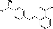
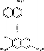
Acid Red 27, a monoazo anionic dye, was obtained from Boyakh Saz Company (Iran) which was a commercial dye and used without further purification. Methyl Red was purchased from Fluka and used without further purification. Table 1 displays the characteristics of these dyes. HCl, H2SO4, NaOH, H2O2 and FeSO4 were obtained from Merck (Germany). Stock solutions Acid Red 27 (200 mg L−1) and Methyl Red (20 mg L−1) were prepared by dissolving the requisite quantity of the dye in HCl 0.001 M. FeSO4 was prepared as a 0.1 M solution in 1 mM H2SO4 solution.| Dye | Chemical Structure | Molecular Formula | Color Index Number | λ max (nm) | M w (g mol−1) |
|---|---|---|---|---|---|
| MR |
|
C15H15N3O2 | 13020 | 520 | 269.30 |
| AR 27 |
|
C20H14N2O10S3 | 16185 | 525 | 604.48 |
3.3. Calibration and validation set
Two sets of standard solutions, calibration and validation sets, were prepared. 25 samples of calibration mixtures of two dyes were designed using 5 levels full factorial design. Appropriate volumes of the standard solutions were prepared in HCl 0.001 M. The concentrations of each compound in the resulting solutions were in the dynamic linear range of 10.0–100.0 and 1.0–10.0 mg L−1 for Acid Red 27 and Methyl Red, respectively. Another 9 samples were designed using 3 levels full factorial design as a validation set. The levels of the concentration of dyes in these samples are shown in Table 2. The compositions of the most concentrated solutions were selected so that the absorbances did not exceed the highest absorbance reading of the instrument. After recording of spectra for each sample, an augmented matrix Daug,1 was constructed appending in the column-wise direction, a matrix D1 that contained the spectra of the 25 standards solutions as a calibration set and a matrix D2 that contained the spectra of 9 mixture solutions of dyes as synthetic unknown samples (validation set).| Data set | Concentration of Methyl Red (mg L−1) | Concentration of Acid Red 27 (mg L−1) |
|---|---|---|
| Calibration set | 1.0, 2.0, 3.0, 4, 5 | 10.0, 20.0, 30.0, 40.0, 50.0 |
| Validation set | 2.5, 3.5, 4.5 | 25.0, 35.0, 45.0 |
3.4. Experimental design
In the present study, central composite design was employed for the modeling of the Fenton process. In order to evaluate the influence of operating parameters on the decolorization efficiency of two dyes, four influential factors were chosen: initial MR concentration (X1), initial AR 27 concentration (X2), initial H2O2 concentration (X3) and initial Fe(II) concentration (X4). A total of 29 experiments were ran in this work, including 24 = 16 factorial points, 8 axial points (star points) and 5 replications at the center point. Experimental data were analyzed using Minitab 15 software. The experimental ranges and the levels of the independent variables for two dyes removal are given in Table 3.| Factor | Coded levels | ||||
|---|---|---|---|---|---|
| −2 | −1 | 0 | +1 | +2 | |
| C MR (X1) (mg L−1) | 1 | 2 | 3 | 4 | 5 |
| C AR 27 (X2) (mg L−1) | 10 | 20 | 30 | 40 | 50 |
| C H2O2 (X3) (mg L−1) | 1 | 2 | 3 | 4 | 5 |
| C Fe(II) (X4) (mM) | 0.5 | 1 | 1.5 | 2 | 2.5 |
3.5. Procedure
The decolorization experiments were performed in a beaker maintained in a dark environment. Appropriate volumes of stock solutions of dye and FeSO4 were poured into 100 mL Florence flasks and diluted with distilled water to 100 mL. The pH of the solutions was adjusted to 3.0 using a dilute solution of sulfuric acid while using a pH meter. The reactions were initiated by adding an appropriate predetermined amount of hydrogen peroxide to the beaker. All experiments were sampled using a pipette after 12 min and were analyzed spectrophotometrically. The concentrations of the remaining dyes were determined using the proposed MCR-ALS method. The efficiency of the Fenton reaction in removing of dyes was calculated using eqn (5). | (5) |
3.6. Spiked samples
In order to test the performance of the proposed chemometric method in determination of the dye concentrations, the mixture of two dyes was treated using the Fenton reaction and the remaining solutions were used as wastewater samples.During the reaction, in the first 12 min, samples were taken every 2 min and were used as wastewater samples. Then, their spectra were recorded. Finally, different amounts but known values of the standard of dyes were added to them and used as spiked samples. The spectra of the spiked samples were recorded.
4. Results and discussion
In order to find the linear dynamic range of the dyes, the absorbance of AR 27 and MR was measured at 525 and 520 nm, respectively. Individual curves were evaluated by linear regression by plotting absorbance against the concentration of AR 27 and MR in the range of 10–100 and 1–10 mg L−1, respectively. The characteristics of the calibration graph and the statistical parameters for determination of AR 27 and MR are summarized in Table 4. As the selected wavelengths used for the individual calibration of each compound were not selective, so the results shown in Table 4 could not be used for determination of these two compounds in the mixed solutions. But linear dynamic ranges of analytes can be used to construct the calibration set in multivariate calibration.| Parameters | Methyl Red | Acid Red 27 |
|---|---|---|
| λ max (nm) | 520 | 525 |
| Dynamic linear range (mg L−1) | 1–10 | 10–100 |
| Correlation coefficient | 0.9973 | 0.9966 |
| Limit of detection (μg mL−1) | 0.21 | 3.15 |
| Equation of calibration curve (n = 5) (absorbance versus mg L−1 of analyte) | A = 0.1876C + 0.0077 | A = 0.0227C + 0.0717 |
The lack of bilinearity and additivity of data are some of the difficulties in the application of multivariate calibration methods. Therefore, the linearity and additivity of spectrophotometric responses were investigated. Fig. 1 shows the individual spectra, mixture and sum of the spectra for AR 27 and MR. As can be seen from the figure, there is not any interaction between analytes. Also the signals have good additive properties.
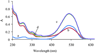 | ||
| Fig. 1 Absorption spectra of (a) MR (2 mg L−1), (b) AR (10 mg L−1), (c) their mixture with the same concentration and (d) theoretical mixture of two dyes. | ||
As mentioned previously, MCR-ALS is a powerful tool for the species resolution and quantitative determination of many types of unresolved chemical mixtures. This method is able to determine analytes in the presence of unknown interferents (second order advantage). So in the present work, MCR-ALS was used as a multivariate calibration method.
For quantification, the data matrices corresponding to the unknown samples and those of the standards have to be analyzed simultaneously. So, the resolution was performed using the strategy of the augmented matrices.35 An augmented matrix Daug,1 was constructed by column wise augmentation of D1 and D2 which contained the spectra of 25 standards solutions as a calibration set and the spectra of 9 mixture solutions of dyes as synthetic unknown samples (validation set), respectively.
An another augmented matrix Daug,2 was constructed by column wise augmentation of D1, D2 and D3. D3 is a matrix containing the spectra recorded during the Fenton process that are shown in Fig. 2.
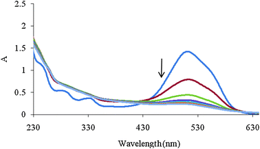 | ||
| Fig. 2 Spectra of mixture solution during Fenton process with 2 min intervals. Initial concentrations of MR, AR 27, H2O2 and Fe(II) were 4 mg L−1, 40 mg L−1, 6 mg L−1 and 2 mM, respectively. | ||
The number of chemical species present in the augmented matrix was first estimated by eigenvalue analysis, since it was assumed that the eigenvalues associated to the chemical components were much larger than the other possible contributions such as instrumental drift or experimental error. Therefore, the chemical rank was estimated by simply inspecting the tables of eigenvalues and ratios of the consecutive eigenvalues of the augmented matrices. The ratio of the consecutive eigenvalues of Daug,1 reaches a maximum at i = 2, indicating that two absorbing species exist in the considered matrix. But the ratio of the consecutive eigenvalues of Daug,2 reaches a maximum at i = 3, indicating that three absorbing species exist in the considered matrix. This observation can be attributed to the presence of a by-product of the Fenton reaction. Degradation of Acid Red 27 has been studied by the Fenton reaction, previously41 and an absorptive compound was not reported for it. But it is not possible to say surely that there is only one component because it is possible two components are produced during decolorization and they are collinear so it is not possible to resolve them by MCR. The collinearity problem is usual in resolving complex systems where two or more reactions progress simultaneously. In such cases it is possible that the produced components are linearly dependent so the resolved spectrum for the products is a linear combination of their spectra. So the green curve (c) in Fig. 3A and 3B maybe is a linear combination of pure profiles of the products and is not related to only one component.
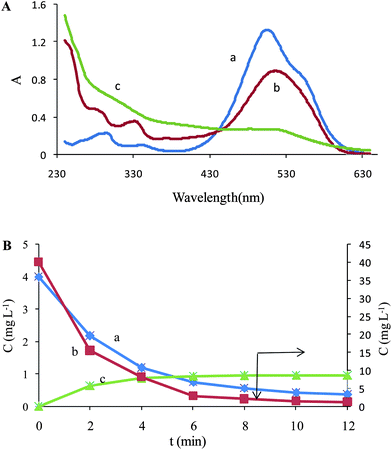 | ||
| Fig. 3 (A) Resolved spectra for Daug,2 (a) MR, (b) AR 27 and (c) unknown component. (B) Concentration profiles of (a) MR, (b) AR 27 and (c) unknown component in the Fenton process. | ||
Since the spectra for AR 27 and MR standard solutions were available, so the optimization step of MCR-ALS was initiated using the spectra of the individual components ST in the resolving of Daug,1. But, in the resolving of Daug,2, to improve the resolution, we added a vector corresponding to the last degradation time at which the third component was predominant over the dyes studied.
A series of constraints was applied in an attempt to improve the optimization and to restrict the number of possible solutions: (a) the spectra of each component must be non-negative; (b) the concentration profiles of each component must be non-negative, (c) since the concentration for AR 27 and MR standard solutions (calibration set) were available, the algorithm was forced (as an equality constraint) to keep these concentrations for the dyes during the MCR-ALS optimization. The applied equality constraint, which consists of fixing the concentration of the dyes in standard samples during the optimization process, contributed to break-up the ambiguities that are intrinsic to the MCR-ALS methods. In this way, quantitative results could be obtained.
It is important to note that the second order advantage is achieved by simultaneously analyzing the calibration data and the samples data. This large data set, Daug,2, was decomposed into contributions from the analytes and the potential interferences, and prediction was made. Fig. 3 shows the recovered spectra in the matrix ST after the ALS optimization. Besides the spectra of AR 27 and MR, the spectra corresponding to the interferent was recovered. There is a little difference between spectrum of MR (Fig. 1) and resolved profile that can be attributed to the ambiguity of MCR.
Spiked samples were used to check the accuracy of the proposed method. The above mentioned wastewater sample was spiked with different amounts of two dyes. The spectra of the spiked samples were augmented with standard solution's spectra to get Daug,3. Daug,3 was resolved to determine the concentrations. The average of recoveries and relative standard errors (RSE) (eqn (6)) were calculated for estimated concentrations of the dyes using the proposed algorithm.
 | (6) |
The results are summarized in Table 5. As can be seen, satisfactory results were obtained for each dye. The developed MCR-ALS method allows the concentrations of two dyes to be determined despite their spectra overlapping. So this method can be used to monitor the decolorization efficiency of the mixture of these dyes using the Fenton reaction.
Response surface methodology such as central composite design was used to assemble the model in order to describe the way in which the variables are related and influence the response. In this study, four independent variables including concentration of MR (X1), concentration of AR (X2), concentration of H2O2 (X3) and concentration of Fe(II) (X4) were studied at five levels. The preliminary experiments were performed to determine the extreme values of the variables. The coded levels of the variables and their real experimental values are given in Table 3. Also, as it is very important to estimate pure experimental uncertainty, the central point was repeated five times. Therefore, twenty nine experiments were randomized, in order to minimize the effect of uncontrolled variables. Twelve minutes after starting a reaction, spectra of the solutions were recorded in each experiment. The concentrations of each dye in the mixture were determined using the proposed MCR-ALS method. The 4-factor CCD matrix and experimental results obtained in the decolorization runs are presented in Table 6. The data obtained from the set of conditions employed by the central composite design were fitted to eqn (4) (full second-order polynomial). It is always necessary to examine the fitted model to ensure that it provides an adequate expectedness to the true system. The model is only validated when it shows a good predictability. The model adequacy can be assessed by the employment of different statistical tools. The most powerful numerical method for model validation is by the application of analysis of variance (ANOVA), which is based on a decomposition of the total variability in the selected response (Y). It checks the adequacy of the regression model in terms of a lack-of-fit test. The lack-of-fit was meaningless for the regression (p > 0.05 at a 95% confidence level). The square of correlation coefficient (R2) quantitatively measures the correlation between the experimental data and the predicted responses. R2 was 0.9106 and 0.8745 for AR 27 and MR, respectively. The model predictability can be determined from the graphical point of view by a normal probability plot of residuals and histogram of residuals. The normal probability plots for degradation of both dyes were linear. All these results showed that the proposed models were valid in the prediction of responses.
| Run No. | C MR (mg L−1) | C AR 27 (mg L−1) | C H2O2 (mg L−1) | C Fe(II) (mM) | Y AR 27 (%) | Y MR (%) |
|---|---|---|---|---|---|---|
| 1 | 2 | 20 | 2 | 1 | 17.44 | 32.02 |
| 2 | 4 | 20 | 2 | 1 | 10.81 | 25.04 |
| 3 | 2 | 40 | 2 | 1 | 21.75 | 39.30 |
| 4 | 4 | 40 | 2 | 1 | 22.07 | 4.80 |
| 5 | 2 | 20 | 4 | 1 | 17.87 | 16.47 |
| 6 | 4 | 20 | 4 | 1 | 10.74 | 34.38 |
| 7 | 2 | 40 | 4 | 1 | 16.99 | 47.19 |
| 8 | 4 | 40 | 4 | 1 | 8.79 | 36.91 |
| 9 | 2 | 20 | 2 | 2 | 60.35 | 68.70 |
| 10 | 4 | 20 | 2 | 2 | 32.94 | 60.30 |
| 11 | 2 | 40 | 2 | 2 | 17.81 | 12.33 |
| 12 | 4 | 40 | 2 | 2 | 5.33 | 2.75 |
| 13 | 2 | 20 | 4 | 2 | 55.88 | 80.49 |
| 14 | 4 | 20 | 4 | 2 | 43.70 | 78.71 |
| 15 | 2 | 40 | 4 | 2 | 21.85 | 46.74 |
| 16 | 4 | 40 | 4 | 2 | 16.22 | 27.10 |
| 17 | 1 | 30 | 3 | 1.5 | 27.25 | 67.20 |
| 18 | 5 | 30 | 3 | 1.5 | 12.33 | 50.97 |
| 19 | 3 | 10 | 3 | 1.5 | 54.39 | 88.99 |
| 20 | 3 | 50 | 3 | 1.5 | 18.08 | 16.05 |
| 21 | 3 | 30 | 1 | 1.5 | 26.83 | 25.72 |
| 22 | 3 | 30 | 5 | 1.5 | 16.56 | 49.91 |
| 23 | 3 | 30 | 3 | 0.5 | 6.15 | 10.79 |
| 24 | 3 | 30 | 3 | 2.5 | 37.42 | 60.60 |
| 25 | 3 | 30 | 3 | 1.5 | 21.48 | 47.47 |
| 26 | 3 | 30 | 3 | 1.5 | 20.49 | 44.34 |
| 27 | 3 | 30 | 3 | 1.5 | 25.77 | 41.44 |
| 28 | 3 | 30 | 3 | 1.5 | 25.79 | 41.70 |
| 29 | 3 | 30 | 3 | 1.5 | 22.84 | 43.73 |
In order to gain insight about the effect of variables, three dimensional (3D) and contour (2D) plots were formed to analyze the change of the response for the predicted responses. The contour plots of the quadratic model with two variables kept constant at their zero level and the other two varying within the experimental ranges are shown in Fig. 4–6. These plots provide a method to predict the decolorization efficiency for different values of the tested variables and help to identify the type of interactions between these variables.
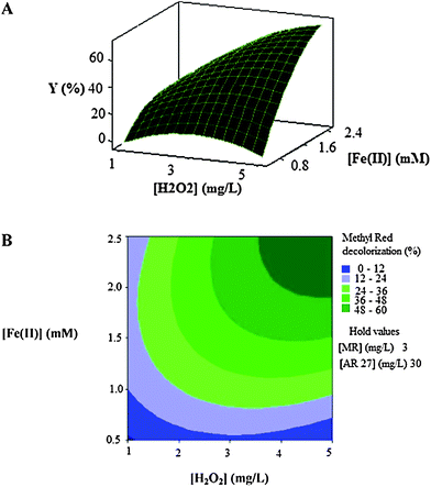 | ||
| Fig. 4 The response surface (A) and contour plot (B) of the decolorization efficiency (%) of MR as the function of the initial concentration of Fe(II) (mM) and initial H2O2 concentration (mg L−1). | ||
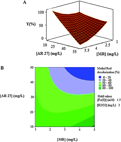 | ||
| Fig. 5 The response surface (A) and contour plot (B) of the decolorization efficiency (%) of MR as the function of the initial concentration of dyes (mg L−1). | ||
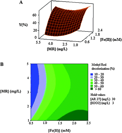 | ||
| Fig. 6 The response surface (A) and contour plot (B) of the decolorization efficiency (%) of MR as the function of the initial concentration of Fe(II) (mM) and initial dye's concentration (mg L−1) of MR. | ||
Fig. 4A and Fig. 4B show that the decolorization efficiency increases with the increase in the initial concentrations of catalyst (Fe(II)) and oxidant (H2O2). The maximum efficiencies are got in high levels of concentrations of two factors.
As can be seen in Fig. 5A and Fig. 5B, the decolorization efficiency decreases with the increase in the initial concentrations of the two dyes and the minimum efficiencies are achieved in high levels of concentrations of the two dyes when the other two factors, initial concentrations of catalyst (Fe(II)) and oxidant (H2O2), are held constant at 1.5 mg L−1 and 3 mg L−1, respectively.
Fig. 6A and Fig. 6B show the effect of the initial concentration of the catalyst (Fe(II)) and dye on the decolorization efficiency. It is clear that there are significant interactions between the two factors because the effects of one of them differ by changing the level of the other one.
The obtained models for decolorization of two dyes using CCD were validated with 16 experiments with different initial concentrations of AR 27, MR, H2O2 and Fe(II) that had been orthogonally designed. Then decolorization efficiencies (Yexperimental) were obtained after recording spectra and analysis by the proposed MCR method. Also, decolorization efficiencies were calculated using the obtained quadratic equation by CCD (Ypredicted). Fig. 7 shows the results of plotting Yexperimentalversus Ypredicted. The obtained values of the square of the correlation coefficient were included to show the fitting quality of all data to a straight line. The results showed that the proposed models were successful in predicting the decolorization efficiency.
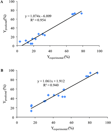 | ||
| Fig. 7 Plotting of the Yexperimental (%) versus Ypredicted (%) for validation set (A) AR 27 and (B) MR. | ||
5. Conclusions
The determination of Methyl Red and Acid Red 27 was successfully performed in binary mixtures of the dyes by combined direct UV-vis spectrophotometric measurements and multivariate curve resolution-alternating least squares method. The proposed method was used as a monitoring system for removing these dyes using Fenton reaction. Also, central composite design has been applied to model the decolorization of the dye solution containing two dyes using the Fenton process. The effect of experimental parameters on the decolorization efficiency was established by the response surface and contour plots of the model-predicted responses.Acknowledgements
The authors are most grateful for the continuing financial support of this research project by the University of Tabriz.References
- B. K. Körbahti and M. A. Rauf, Chem. Eng. J., 2008, 136, 25 CrossRef.
- C. Hachem, F. Bocquillon, O. Zahraa and M. Bouchy, Dyes Pigm., 2001, 49, 117 CrossRef CAS.
- M. M. Nassar and Y. H. Magdy, Chem. Eng. J., 1997, 66, 223 CrossRef CAS.
- H. Ben Mansour, D. Barillier, D. Corroler, K. Ghedira, L. Chekir-Ghedira and R. Mosrati, Environ. Toxicol. Chem., 2009, 28, 489 CrossRef CAS.
- M. N. Chong, B. Jin, C. W. K. Chow and C. Saint, Water Res., 2010, 44, 2997 CrossRef CAS.
- E. G. Garrido-Ramirez, B. K. G. Theng and M. L. Mora, Appl. Clay Sci., 2010, 47, 182 CrossRef CAS.
- A. R. Khataee, V. Vatanpour and A. R. Amani Ghadim, J. Hazard. Mater., 2009, 161, 1225 CrossRef CAS.
- A. R. Khataee and G. Dehghan, J. Taiwan Inst. Chem. Eng., 2011, 42, 26 CrossRef CAS.
- N. Daneshvar, D. Salari and A. R. Khataee, J. Photochem. Photobiol., A, 2003, 157, 111 CrossRef CAS.
- J. J. Pignatello, E. Oliveros and A. MacKay, Crit. Rev. Environ. Sci. Technol., 2006, 36, 1 CrossRef CAS.
- E. Neyens and J. Baeyens, J. Hazard. Mater., 2003, 98, 33 CrossRef CAS.
- M. A. Behnajady, N. Modirshahla and F. Ghanbary, J. Hazard. Mater., 2007, 148, 98 CrossRef CAS.
- A. C. V. dos Santos and J. C. Masini, Microchem. J., 2009, 93, 110 CrossRef CAS.
- R. G. Zepp, B. C. Faust and J. Hoigne, Environ. Sci. Technol., 1992, 26, 313 CrossRef CAS.
- A. K. Gupta, A. Pal and C. Sahoo, Dyes Pigm., 2006, 69, 224 CrossRef CAS.
- A. R. Khataee, M. Zarei, M. Fathinia and M. K. Jafari, Desalination, 2011, 268, 126 CrossRef CAS.
- K. Sahel, N. Perol, F. Dappozze, M. Bouhent, Z. Derriche and C. Guillard, J. Photochem. Photobiol., A, 2010, 212, 107 CrossRef CAS.
- M. Mkandawire, J. Förster, D. Fiedler, H. Böttcher and W. Pompe, Int. J. Environ. Anal. Chem., 2009, 89, 529 CrossRef CAS.
- C. Fernandez, M. S. Larrechi and M. P. Callao, TrAC, Trends Anal. Chem., 2010, 29, 1202 CrossRef CAS.
- M. M. Galera, M. D. G. García and H. C. Goicoechea, TrAC, Trends Anal. Chem., 2007, 26, 1032 CrossRef CAS.
- C. Fernández, M. S. Larrechi and M. P. Callao, J. Hazard. Mater., 2010, 180, 474 CrossRef.
- C. Fernández, M. S. Larrechi and M. P. Callao, Talanta, 2009, 79, 1292 CrossRef.
- A. Naseri and H. Abdollahi, Anal. Methods, 2011, 3, 429 RSC.
- M. A. Bezerra, R. E. Santelli, E. P. Oliveira, L. S. Villar and L. A. Escaleira, Talanta, 2008, 76, 965 CrossRef CAS.
- A. R. Khataee and G. Dehghan, J. Taiwan Inst. Chem. Eng., 2011, 42, 26 CrossRef CAS.
- H. S. Li, S. Q. Zhou, Y. B. Sun and J. A. Lv, Waste Manage., 2010, 30, 2122 CrossRef CAS.
- S. Mohajeri, H. A. Aziz, M. H. Isa, M. A. Zahed and M. N. Adlan, J. Hazard. Mater., 2010, 176, 749 CrossRef CAS.
- A. R. Khataee and B. Habibi, Desalin. Water Treat., 2010, 16, 243 CrossRef CAS.
- R. Tauler, A. Izquierdo-Ridorsa and E. Casassas, Chemom. Intell. Lab. Syst., 1993, 18, 293 CrossRef CAS.
- R. Tauler, A. Smilde and B. Kowalski, J. Chemom., 1995, 9, 31 CrossRef CAS.
- A. De Juan and R. Tauler, Crit. Rev. Anal. Chem., 2006, 36, 4 CrossRef.
- J. Diewok, A. de Juan, M. Maeder, R. Tauler and B. Lendl, Anal. Chem., 2003, 75, 641 CrossRef CAS.
- H. C. Goicoechea, A. C. Olivieri and R. Tauler, Analyst, 2010, 135, 636 RSC.
- J. Jaumot, R. Gargallo, A. de Juan and R. Tauler, Chemom. Intell. Lab. Syst., 2005, 76, 101 CrossRef CAS.
- R. Tauler, Chemom. Intell. Lab. Syst., 1995, 30, 133 CrossRef CAS.
- E. Morgan, Chemometrics: Exprimental Design, John Wiley, London, 1991 Search PubMed.
- J. N. Miller and J. C. Miller, Statistics and Chemometrics for Analytical Chemistry, Pearson Education, Harlow, 2005 Search PubMed.
- A. R. Khataee, Environ. Technol., 2010, 31, 73 CrossRef CAS.
- S. Gorji and M. Bahram, Anal. Methods, 2010, 2, 949 Search PubMed.
- I. Bulacov, J. Jirkovsky, M. Muller and R. B. Heimann, Surf. Coat. Technol., 2006, 201, 255 CrossRef.
- S. Ledakowicz, R. Maciejewska, L. Gebicka and J. Perkowski, Ozone: Sci. Eng., 2000, 22, 195 CrossRef CAS.
| This journal is © The Royal Society of Chemistry 2012 |
