High precision Mg isotope measurements of meteoritic samples by secondary ion mass spectrometry

Abstract

The possibility of establishing an accurate relative chronology of the early solar system events based on the decay of short-lived ²⁶Al to ²⁶Mg (half-life of 0.72 Myr) depends on the level of homogeneity (or heterogeneity) of ²⁶Al and Mg isotopes. However, this level is difficult to constrain precisely because of the very high precision needed for the determination of isotopic ratios, typically of ±5 ppm. In this study, we report for the first time a detailed analytical protocol developed for high precision in situ Mg isotopic measurements (²⁵Mg/²⁴Mg and ²⁶Mg/²⁴Mg ratios, as well as ²⁶Mg excess) by MC-SIMS. As the data reduction process is critical for both accuracy and precision of the final isotopic results, factors such as the Faraday cup (FC) background drift and matrix effects on instrumental fractionation have been investigated. Indeed these instrumental effects impacting the measured Mg-isotope ratios can be as large or larger than the variations we are looking for to constrain the initial distribution of ²⁶Al and Mg isotopes in the early solar system. Our results show that they definitely are limiting factors regarding the precision of Mg isotopic compositions, and that an under- or over-correction of both FC background instabilities and instrumental isotopic fractionation leads to important bias on δ²⁵Mg, δ²⁶Mg and Δ²⁶Mg values (for example, olivines not corrected for FC background drifts display Δ²⁶Mg values that can differ by as much as 10 ppm from the truly corrected value). The new data reduction process described here can then be applied to meteoritic samples (components of chondritic meteorites for instance) to accurately establish their relative chronology of formation.

---

1 Introduction

Variations of the Mg isotopic composition of meteoritic materials can be understood at first order to be the sum of (i) mass-dependent isotopic fractionations due to processes such as evaporation or condensation and (ii) the decay of short-lived ²⁶Al to ²⁶Mg (half-life of 0.72 Myr). Calcium-, aluminum-rich inclusions (CAIs), that are the oldest dated solids formed in the accretion disk around the early sun,^1–3 display large ²⁶Mg excesses.⁴ They can be used to define the initial ²⁶Al/²⁷Al ratio (5.23 (±0.13) × 10⁻⁵ (ref. 5 and 6)) that anchors the ²⁶Al-based chronology. However, the ²⁶Al–²⁶Mg system can be used as a chronometer only under the assumption that ²⁶Al and Mg isotopes were homogenized early in the accretion disk.

The level of homogeneity (or heterogeneity) is difficult to constrain precisely. One way is to be able to compare ²⁶Mg excesses measured with high precision in samples formed at various ages in the accretion disk with ²⁶Mg excesses predicted assuming homogeneity. For a solar ²⁷Al/²⁴Mg ratio of 0.101 (ref. 7) (this ratio being estimated from CI chondrites, and not the solar photosphere), ²⁶Mg produced from the total decay of an initial ²⁶Al/²⁷Al ratio of 5.23 × 10⁻⁵ increases the ²⁶Mg/²⁴Mg ratio by ∼38 ppm. The magnitude of ²⁶Mg excesses measured in situ by MC-SIMS (multi-collection secondary ion mass spectrometry) in ferromagnesian chondrules (chondrules are mm sized objects which were melted and quenched in the accretion disk and they constitute the major high-temperature component of primitive meteorites) from ordinary chondrites does support a ±10% homogeneous distribution of ²⁶Al and Mg isotopes at the time of CAI formation in the disk.⁸ This view has been challenged⁹ from very high precision bulk analyses (±2.5 ppm for ²⁶Mg excesses¹⁰) of refractory components of carbonaceous chondrites (CAIs and amoeboid olivine aggregates) by HR-MC-ICPMS (high-resolution multi-collector inductively coupled plasma source mass spectrometry).

One key to the debate is the development of high precision for Mg isotopic measurements, both bulk and in situ. In fact, the studied objects (i.e. CAIs) underwent, after their formation from precursors condensed from the gas, several high temperature events including melting and re-crystallization. If melting/crystallization occurred in a closed system, it did not modify the bulk compositions (Mg and Al isotopes and Al/Mg ratio) so that a bulk ²⁶Al isochron gives theoretically access to the Al and Mg isotopic compositions of the precursors and thus dates condensation. At variance in situ analysis by MC-SIMS allows us to look for the existence of a ²⁶Al mineral isochron within one object, which would date the partitioning of Al and Mg between the different constituent minerals during the last melting/crystallization event. The combination of bulk and in situ data should allow us to reconstruct the history of the high temperature components of meteorites, from early condensation events to late melting and re-melting processes.

A high precision Mg isotopic measurement method has already been developed for HR-MC-ICPMS.¹⁰ However, bulk analyses by HR-MC-ICPMS require a large sample size and do not allow us to determine mineral isochrons because of the high spatial resolution required in the case of the early solar system objects.

Here we describe the analytical protocol developed for high precision Mg isotopic measurements (²⁵Mg/²⁴Mg and ²⁶Mg/²⁴Mg ratios, as well as ²⁶Mg excess) of meteoritic samples by MC-SIMS on ∼30–40 μm analytical spots. This protocol is a further refinement of that developed by Villeneuve et al.^8,11 Other groups are developing these measurements^12–15 but their procedure is not yet described in full detail. The factors limiting the precision are assessed. An example of application to the study of several components of chondritic meteorites is given.

2 Data acquisition

Mg-isotope ratios and Al/Mg ratios are measured using the CRPG-CNRS (Nancy) CAMECA large radius ims 1270 and ims 1280HR2 ion microprobes (some instrument configuration and capabilities of MC-SIMS can be found in Benninghoven et al.¹⁶ and de Chambost¹⁷). Gold coated or carbon coated polished thick sections of samples are sputtered by a 13 kV O⁻ static primary beam and positive secondary ions of Al and Mg isotopes are extracted and accelerated at 10 kV. The intensity of the primary beam is set to produce the highest possible count rate for secondary ions (i.e. >1 × 10⁹ counts per second (cps) on ²⁴Mg⁺, in olivines), while keeping the beam diameter small enough to allow the analysis of individual mineral phases in chondrules or CAIs: for instance a ∼30 nA primary beam intensity corresponds to a ∼30–40 μm spot size. The secondary ions are analyzed at a mass resolution M/ΔM = 2500 (using exit slit #1 of the multicollector) in multicollection mode using four Faraday cups (FCs): L′2, C, H1 and H′2, for ²⁴Mg, ²⁵Mg, ²⁶Mg and ²⁷Al, respectively. Such a low mass resolution is chosen to maximize the flatness of the three Mg peaks though the interference of the hydride ²⁴MgH⁺ on ²⁵Mg (with vacuum in the sample chamber below 3 × 10⁻⁹ Torr, the contribution of ²⁴MgH⁺ to ²⁵Mg is less than 10⁻⁶ relative) is not totally resolved (a M/ΔM of 3559 would be required). However measurements made at higher mass resolution (M/ΔM = 6000 using exit slit #2) have shown that the contribution of the hydride to ²⁵Mg remains less than a few cps, i.e. <∼10⁻⁸ relative for ²⁵Mg (whose intensity is greater than a few 10⁸ cps in olivines) if the vacuum in the chamber is <3 × 10⁻⁹ Torr.

Each analysis of a new sample mount starts by a manual setting of the Z position of the mount to keep constant the distance between the sample surface and the front plate of the immersion lens. When possible, different grains of different international and in-house standards are included with the sample(s) to analyze in the same mount. In addition, different mounts containing standards are also analyzed in between mounts containing samples and standards. Generally, analyses are automatically chained. A chain of analyses can include both depth profiles (in that case no more than 7 measurements are done at the same spot) and analyses at different spots on a same grain or on different grains (standard or sample) close to each other in the mount (in that case the sample stage is moved, only over a short distance, but allowing much more analyses to be done, the number depending on the spot size). Whatever the case the primary beam never moves. One typical analysis lasts for 425 s, including a total of 150 s presputtering and 275 s simultaneous counting of the intensities of ²⁴Mg⁺, ²⁵Mg⁺, ²⁶Mg⁺ and ²⁷Al⁺ (25 cycles of 10 s counting time separated by 1 s waiting time). During presputtering, first the background of each FC is measured (the secondary beam is deflected from the entrance of the magnet by the deflector Y of the coupling lens LC1C) and, second, an automatic centering of the secondary beam is performed (using secondary intensity measured for ²⁴Mg) either in the field aperture (using transfer lenses deflectors LTdefxy) with the ims 1270 or in both the field aperture and the contrast aperture (using transfer lenses deflectors DTFAxy and DTCAxy) with the ims 1280HR2. This automatic centering allows the correction of the secondary beam trajectory for possible small deviations due to imperfect alignment or flatness of the sample. In addition to these centerings, the charging of the sample is automatically monitored (and the secondary high voltage readjusted of a few volts if necessary) by scanning the energy distribution of secondary ions. The nuclear magnetic resonance (NMR) field sensor is used on the ims 1280HR2 to control and stabilize the magnetic field since no peak jumping is required because of the use of multi-collection.

3 Data reduction

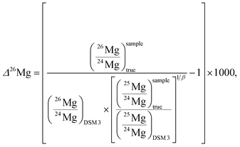
At the level of precision required for Mg isotope analysis of extraterrestrial materials (e.g. 10 ppm or better on ²⁶Mg excesses noted Δ²⁶Mg, see Section 3.5 for definition) the procedure of data reduction is critical to avoid introduction of any analytical bias in the final isotopic results. This is particularly critical for MC-SIMS analysis for two major reasons. First, in MC-SIMS all measurements are direct measurements of isotopic compositions while in HR-MC-ICPMS, thanks to the standard–sample bracketing technique which cannot be used for SIMS, only differences of isotopic compositions are measured, thus eliminating most of the instrumental isotopic fractionations. Second, significant matrix effects are present and have a major influence on instrumental fractionation. However, MC-SIMS has the advantage of a much lower instrumental fractionation, one order of magnitude less, than HR-MC-ICPMS. The approach developed to calibrate precisely and to correct for instrumental fractionation is described in the following, as well as the propagation of errors due to these different corrections.

In the following, Mg isotopic compositions will be expressed either as isotopic ratios or as delta values. The δ^25,26Mg notation is the relative deviation, in per mil (‰), of the ^25,26Mg/²⁴Mg ratio from a reference isotopic composition (noted (δ^xMg)_{DSM 3} when the DSM 3 international standard is used).

where x stands for 25 or 26.

The reference isotopic composition used to calculate the raw Mg-isotope ratios is that of SRM 980, with ²⁵Mg/²⁴Mg = 0.12663 and ²⁶Mg/²⁴Mg = 0.13932,¹⁸ because the DSM 3 Mg-isotope ratios are determined relative to the SRM 980 international standard. A re-evaluation of these ratios has recently been published (²⁵Mg/²⁴Mg = 0.126896 and ²⁶Mg/²⁴Mg = 0.139652 (ref. 10)). However, as explained in the following, because most of the data reduction is made using isotopic ratios and not delta values, and because instrumental fractionation is calibrated from the analyses of different standards, the final corrected delta values are independent of the values taken as the reference isotopic ratios.

The capital delta notation (Δ²⁶Mg, in ‰) will also be used hereafter to express ²⁶Mg excesses or deficits relative to a given mass fractionation law. In the case of a mass fractionation law for Mg isotopes characterized by a coefficient of 0.521 (see Section 3.5 for more details), the Δ²⁶Mg value is calculated according to:

Note that Ogliore et al.¹⁹ have recently shown that in SIMS the mean of isotopic ratios determined from individual measurement cycles at low count rates is biased, yielding a long-run averaged ratio that is systematically higher than the true ratio. However, this effect is completely negligible at the high count rates used to measure the Mg-isotope ratios discussed in this paper.

3.1 Raw data and outlier rejection

The measured isotopic ratios averaged over 25 cycles and corrected only for the yields (determined from the Cameca calibration routine²⁰ at the beginning of each analytical session) and the backgrounds (determined during pre-sputtering) of the four Faraday cups are named raw data (e.g. (²⁵Mg/²⁴Mg)_raw). Several instrumental parameters are automatically registered with the raw data. Thus for each measurement raw data are accompanied by (i) the x and y sample positions (in μm) and a picture of the sample in reflected light through the ion probe microscope at the beginning of sputtering, (ii) the sample chamber pressure (in Torr), (iii) the primary beam intensity (in A), (iv) the transfer deflectors values (LTdefxy for the ims 1270; DTFAxy and DTCAxy for the ims 1280HR2) which are automatically centered, (v) the drift of the secondary high voltage (in V) which is determined automatically, (vi) the background of the four FCs (in cps), (vii) the secondary intensities of ²⁴Mg⁺, ²⁵Mg⁺, ²⁶Mg⁺ and ²⁷Al⁺ (in cps), (viii) the ²⁵Mg/²⁴Mg, ²⁶Mg/²⁴Mg and ²⁶Mg/²⁵Mg isotopic ratios, expressed in the δ^xMg notation (with x = 25 or 26 for ratios to ²⁴Mg) with their associated 1σ error (1 s.e., n = 25), a 2 standard deviation (2 s.d.) threshold being used to reject outliers within the 25 cycles (rejections of δ²⁵Mg, δ²⁶Mg and ²⁷Al/²⁴Mg are independent so that rejected δ²⁵Mg and δ²⁶Mg, if any, could correspond to different cycles), and (ix) the ²⁷Al/²⁴Mg ratio and its associated 1σ error.

Results for which anomalies were observed during the analytical procedure were systematically discarded. They are identified from any of the following criteria: (i) secondary intensity normalized to the primary beam intensity lower (by 20% or more) than the typical value observed on standards of similar matrix, (ii) spikes in the background measured for the FCs during pre-sputtering, (iii) anomalous charge (more than 15 V) of the sample (if any, it likely results from an incomplete charge compensation due to ageing of the mount metallization or its local removal when spots are close to each other), (iii) anomalously large re-centering of the transfer deflectors (in excess of ±7 V), (iv) low statistic on either the δ²⁵Mg or δ²⁶Mg values (worse than 0.05‰, 1 s.e.). In addition, the samples are systematically observed after analyses with optical microscopy (or secondary electron microscopy) to discard analyses which would correspond to spots not entirely within a grain or spots touching a crack or an inclusion.

3.2 FC background drift

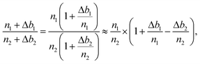
Significant drifts of FC backgrounds take place, primarily due to cyclic temperature variations (worst conditions for the air conditioning system result in an amplitude lower than ±0.4 °C over one day) in the ion probe room. As FC backgrounds are measured during the pre-sputtering at the beginning of each measurement, the raw ²⁵Mg/²⁴Mg and ²⁶Mg/²⁴Mg ratios are systematically corrected for the background drift using a linear interpolation between two successive analyses. Note that the background variations of L′2, H1 and H′2 are correlated within each other, whereas they can be anti-correlated with the background variations of C.

If n₁ and n₂ are two count rates (in cps) for two Mg isotopes and Δb₁ and Δb₂ the drifts (in cps) estimated for their background variations from linear interpolation (Δ = measured background − extrapolated background), then the corrected n₁/n₂ isotope ratio writes:

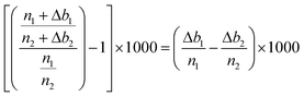
It then comes that the per mil variations of the n₁/n₂ ratio can be expressed as:

So that finally, the delta values can be corrected for the background instabilities according to: 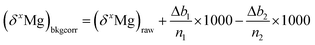, with x = 25 or 26.

Two effects of this correction for drifts of background are significant (Fig. 1). Firstly, because the magnitude of the correction increases when count rates on the different Mg isotopes decrease, this correction will have a larger impact on Mg-poor minerals or glasses or in the case of lower Mg secondary yield. This is the case for pyroxene and spinel relative to olivine. Secondly, because the count rates are about eight times lower on ²⁵Mg and ²⁶Mg relative to ²⁴Mg, the effect of the correction is non-mass dependent and impacts upon the magnitude of the ²⁶Mg excesses that can be calculated from the ²⁵Mg/²⁴Mg and ²⁶Mg/²⁴Mg ratios (with a maximum of 10 ppm change for olivines, Fig. 1).

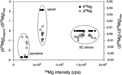Fig. 1 The correction for drifts of Faraday cup backgrounds using a linear interpolation between two successive analyses impacts upon both δ²⁵Mg (black dots) and δ²⁶Mg values (not shown), with a more important effect on Mg-poor minerals (spinel, pyroxene) compared to Mg-rich minerals (olivines for instance). The background correction also affects Δ²⁶Mg values (open squares): this non-mass dependent correction is due to lower count rates on ²⁵Mg and ²⁶Mg compared to ²⁴Mg, with a maximum of 10 ppm change for olivines for instance.

3.3 Instrumental fractionation

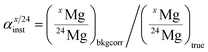
Instrumental isotopic fractionation is produced in SIMS analysis during the extraction and acceleration of secondary ions from the sample, their analysis (transfer optic, electrostatic and magnetic sectors) in the mass spectrometer and their counting in the collectors of the multicollector. Instrumental fractionation resulting from differential breaking of chemical bonds in the sample depending on their vibration energies is a mass-dependent fractionation. Some phenomena which are minor contributors to the isotopic fractionation taking place in the spectrometer can be mass-independent, for example when improper tuning of the transfer optic results in the ²⁴Mg⁺, ²⁵Mg⁺ and ²⁶Mg⁺ ion beams not to be perfectly centered in the cross-over plane where they can be cut differently by the entrance slit of the spectrometer. In addition, improper tuning of the coupling optic (which refocuses the secondary beam between the electrostatic and magnetic sectors) may result in different off-axis aberrations of the secondary beam in the focal plane of the magnet (where the collectors are) and thus in slight differences of peak shapes for the three Mg isotopes and consequently some mass-independent fractionation. Because instrumental isotopic fractionation is primarily mass-dependent, it is generally named instrumental mass fractionation, but one important criterion of proper tuning of the spectrometer is to minimize the mass-independent component of instrumental fractionation, which is indicated by the intercept in its calibration (see below).

Instrumental fractionation (α_inst) is defined for Mg isotopes as:

where x stands for 25 or 26 and the subscripts bkgcorr and true stand for the ratio corrected for drifts of FC background and for the true isotope ratio, respectively. A set of terrestrial reference materials and international standards made of various mantle minerals (San Carlos olivine; Burma spinel; spinel, orthopyroxene and clinopyroxene from a peridotite xenolith from the Vitim volcanic field in Siberia;²¹ orthopyroxene and clinopyroxene from pyroxenites BZCG (also known as BZ-37) and BZ-226 from Zabargad Island in the Red Sea²²) and rocks (CLDR015V, BHVO and BCR2, three terrestrial basalt glasses), and of synthetic glasses (Bacati; glasses of anorthitic, pyroxenic and melilitic (Åk#70) compositions; two NIST SRM glasses²³) is used to determine α_inst (Table 1). Because of the very small variation range of δ²⁶Mg in mantle rocks and high temperature minerals,²⁴ all standard mantle minerals are considered to have the same ²⁶Mg/²⁴Mg and ²⁵Mg/²⁴Mg ratios as San Carlos olivine (δ²⁶Mg_{DSM 3} = −0.25 (±0.04)‰ (2 s.d., n = 29 (ref. 25)), ²⁶Mg/²⁴Mg = 0.1398284 (±0.0000010), ²⁵Mg/²⁴Mg = 0.1268705 (±0.0000005)), but measurements by MC-ICPMS are going on to check that for the few synthetic glasses.

Table 1 Chemical composition for some major elements, and Al/Mg yield, of the terrestrial reference materials and international standards used in this study

Standards	SiO2^e (wt%)	Al2O3^e (wt%)	MgO^e (wt%)	^27Al/^24Mg^e (atomic)	^27Al/^24Mg^f (ion microprobe)	Al/Mg yield
a Chemical composition data coming from this study. b Chemical composition data coming from Decitre (2000). c Chemical composition data coming from Ionov et al. (1993). d Chemical composition data coming from Gao et al. (2002). e Indicates that the 1σ error is typically ±2% for SiO2, Al2O3 and MgO analyses and for the resulting (^27Al/^24Mg)atomic ratio. f Indicates that the 1σ error is typically better than ±1.5% for (^27Al/^24Mg)ion microprobe measurements. g The 1σ error on the Al/Mg yield of Eagle Station olivine is ±0.30.
San Carlos olivine^a	40.33	0.03	48.87	6.14 × 10^−4	4.67 × 10^−4	0.76
Eagle Station (MNHN) olivine^a	39.29	2.72 × 10^−3	42.69	6.37 × 10^−5	6.36 × 10^−5	1.00^g
Clinopyroxene BZCG (Zabargad)^b	50.35	7.05	14.11	0.50	0.38	0.76
Clinopyroxene BZ 226 (Zabargad)^b	51.36	4.49	15.35	0.29	0.23	0.80
Clinopyroxene 313-3 (Vitim)^c	52.84	5.81	15.52	0.37	0.28	0.75
Orthopyroxene BZ 226 (Zabargad)^b	54.14	3.85	31.20	0.12	0.10	0.78
Orthopyroxene 313-3 (Vitim)^c	55.16	3.73	32.94	0.11	0.09	0.77
Spinel (Burma)^a	0.02	71.66	27.88	2.57	1.86	0.72
Spinel 86-1 (Vitim)^c	0.06	57.33	20.9	2.75	2.07	0.75
Basaltic glass MORB CLDR015V^a	50.43	15.83	8.43	1.88	1.41	0.75
Basaltic glass BHVO (Hawaii)^a	49.90	13.50	7.23	1.87	1.41	0.75
Basaltic glass BCR2 (Columbia river)^a	54.10	13.50	3.59	3.76	2.97	0.79
Synthetic anorthitic glass^a	44.05	34.66	1.79	19.41	14.83	0.76
Synthetic melilitic glass^a	41.00	11.00	7.00	1.57	1.10	0.70
Synthetic pyroxenic glass^a	44.38	14.78	11.21	1.32	1.04	0.79
Synthetic glass Bacati^a	31.01	30.74	10.29	2.99	2.41	0.81
Synthetic glass Al20^a	48.68	20.09	9.52	2.11	1.66	0.79
Synthetic glass Al10^a	55.05	10.41	11.37	0.92	0.74	0.81
Synthetic glass Al5^a	58.31	5.11	11.17	0.46	0.38	0.83
Synthetic glass NIST SRM 614^d	71.83	2.29	0.01	435.85	336.90	0.77
Synthetic glass NIST SRM 610^d	69.06	2.20	0.08	28.84	21.82	0.76
Hibonite (Madagascar)^a	0.88	73.70	2.91	25.35	15.95	0.63

---

Matrix effects on instrumental fractionation have been shown to follow a systematic often similar to that observed for natural isotopic fractionations between mineral or between minerals and fluids, as shown for example for D/H in amphiboles and micas.²⁶ By analogy with the exponential law (α^25/24_inst = (α^26/24_inst)^β) generally used²⁷ to express Mg isotopic fractionations for terrestrial or meteoritic samples, the instrumental fractionation law is determined from a linear regression (with the Isoplot 3.00 software²⁸) between ln(α^25/24_inst) and ln(α^26/24_inst) measured for the different international and in-house standards. The instrumental law is always of the following form:²⁹

ln(α^26/24_inst) = [ln(α^25/24_inst) − b]/β_inst

with β_inst varying between 0.51075 and 0.52045 and the intercept b slightly different from 0 with values typically from −0.00058 to −0.00030. Values of β_inst and of b appear to vary independently between different analytical sessions. This instrumental law can be expressed as:

α^25/24_inst = exp(b) × (α^26/24_inst)^β_inst

where it is clear that it differs slightly from a purely mass dependent law because of the term exp(b).

For b very close to 0, one can approximate the above equation by:

α^25/24_inst ≈ (α^26/24_inst)^β_inst.

Large variations of α^25/24_inst due to matrix effects, i.e. caused by variations of vibrational energies of the bonds involving Mg isotopes in minerals or glasses having different chemical compositions, are present among silicates and oxides (Fig. 2). In the case of olivines for instance, a similar effect as previously reported for O isotopes³⁰ exists for Mg isotopes. Values of α^25/24_inst increase by ∼1‰/amu from Fo#79 (olivine from the Eagle Station pallasite) to Fo#88 (San Carlos olivine), and this trend can be linearly extrapolated to determine α^25/24_inst for olivines with Fo# > 88. Similarly for melilite, a change of 1.9‰/amu is observed between two melilite glasses having different Al/Mg ratios. Matrix effects between silicates and oxides are of similar magnitude, e.g. ∼2‰/amu between pyroxene and spinel.

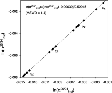Fig. 2 Example of an Mg isotopic instrumental fractionation law, calibrated using reference materials with different compositions (San Carlos olivine, Burma spinel and synthetic pyroxene). Slope and intercept are calculated using the Isoplot 3.00 software.²⁸ Large variations of ln(α^25/24_inst) values are present among silicates and oxides, and are linked to matrix effects which result from variations of vibrational energies of the bonds involving Mg isotopes in minerals or glasses having different chemical compositions.

When the instrumental fractionation law has been properly determined, the (²⁵Mg/²⁴Mg)_bkgcorr ratio of a given sample is corrected for the appropriate value of α^25/24_inst determined from the calibration based on standards with different compositions. Then, the corresponding value of α^26/24_inst is calculated from the instrumental fractionation law (using the values determined for β_inst and b) and is used to correct the (²⁶Mg/²⁴Mg)_bkgcorr ratio. The two Mg-isotope ratios obtained are considered as the “true isotopic ratios” of the sample, in the sense that they are corrected for all ion probe instrumental effects and seem the closest possible to the true values.

3.4 Determination of (δ²⁵Mg)_{DSM 3} and (δ²⁶Mg)_{DSM 3}

The (δ²⁵Mg)_{DSM 3} and (δ²⁶Mg)_{DSM 3} values are calculated from the (²⁵Mg/²⁴Mg)_true and (²⁶Mg/²⁴Mg)_true ratios, respectively (see above), and are expressed with respect to the DSM 3 standard.

The 2σ error on the δ²⁵Mg value of an individual measurement is calculated as the quadratic sum of (i) the external reproducibility determined from repetitive analyses of standards of same matrix as the sample and (ii) the internal error due to the counting statistic according to:

The component which dominates by far in the error is the external reproducibility (typically not better than ±0.150‰ for olivine for instance) which is one order of magnitude higher than the counting statistic error (typically better than ±0.021‰ for olivine for instance). The 2σ error on the δ²⁶Mg value of an individual measurement is calculated similarly.

3.5 Calculation of ²⁶Mg excess or deficit and error propagation

The ²⁶Mg excesses or deficits, written in capital delta notation Δ²⁶Mg (in ‰), are calculated directly from the true isotopic ratios using the following relationship:
with β = β_Earth or β_met (see below), (²⁵Mg/²⁴Mg)_{DSM 3} = 0.126887, (²⁶Mg/²⁴Mg)_{DSM 3} = 0.139863. These ratios were calculated from (δ²⁶Mg)^{DSM 3}_{SRM 980} = 3.90 (±0.03)‰ (2 s.e.), (δ²⁶Mg)^{DSM 3}_{SRM 980} standing for the δ²⁶Mg of DSM 3, expressed with respect to the SRM 980 international standard.^31,32 However, the isotopic homogeneity of the SRM 980 standard has been challenged.³³ Calculation with (δ²⁶Mg)^{DSM 3}_{SRM 980} = 3.40 (±0.13)‰ (ref. 33) results in a 0.007‰ decrease in Δ²⁶Mg values for extraterrestrial materials (that remains within the error bar of the Δ²⁶Mg value calculated with (δ²⁶Mg)^{DSM 3}_{SRM 980} = 3.9‰), whereas no change is seen for terrestrial materials. This is because the β value used to calculate Δ²⁶Mg values for terrestrial samples is 0.521 (β_Earth, corresponding to equilibrium Mg isotopic fractionations³⁴), and 0.514 for meteoritic olivines (β_met).³⁵ This value of 0.514 for β_met has been shown to describe at best most cosmochemical Mg isotope fractionations since they are kinetic, occurring mostly through evaporation and/or condensation processes.^36,37

The 2σ internal error (2 s.e. or 2σ) on Δ²⁶Mg due to counting statistic errors on the ²⁶Mg/²⁴Mg and ²⁵Mg/²⁴Mg ratios is given by:

with β = β_Earth or β_met, and and the errors on the isotope ratios due to counting statistic, typically for an olivine ±0.014‰ and ±0.021‰, respectively. To be conservative, the correlation of errors between the ²⁶Mg/²⁴Mg and ²⁵Mg/²⁴Mg ratios are not taken into account since it could tend to artificially decrease the errors. Note that the relationship between the errors on the isotope ratios and the errors on the delta values is given, for instance for δ²⁵Mg, by:

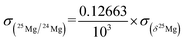
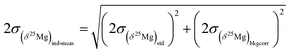
The 2σ error on the Δ²⁶Mg value of an individual measurement is then calculated as the quadratic sum of (i) the external reproducibility determined from repetitive analyses of standards which is of ±0.010‰ for the session shown in Fig. 2 for example, and (ii) the internal error due to the counting statistic according to:

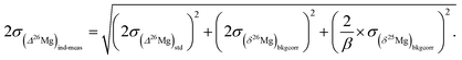
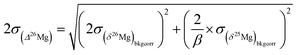
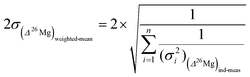
When several measurements (n), e.g. different spots in the same object (such as an isolated olivine or a chondrule), give Δ²⁶Mg values which are identical within ±2σ then a mean Δ²⁶Mg value is calculated for this sample as the weighted mean of the n measurements. The 2σ error associated with this weighted mean is given by:

Finally an important comment must be made concerning the differences between the errors on the δ²⁵Mg and δ²⁶Mg values and the error on the Δ²⁶Mg value. Because variations of mass fractionation follow the instrumental fractionation law (in the three Mg isotopes diagram) they do not introduce errors on Δ²⁶Mg values. Thus for olivines values of are typically of 0.06‰ while values of or are of 0.20‰ and 0.39‰, respectively, for the session shown in Fig. 2. An interesting application of this observation is that several Δ²⁶Mg measurements can be made on a small grain (e.g. <150 μm) successively at the same spot (i.e. by depth profiling). This is a way to improve the precision on the Δ²⁶Mg value when the grain is too small to make several analyses at different locations. Fig. 3b shows the results of seven such depth profiles made on San Carlos olivines (each depth profile corresponds to five to seven successive analyses). Each depth profile gives Δ²⁶Mg values of 0‰ within their 2 s.e. of typically ±0.015‰ (the 2 s.d. for each spot varying from 0.028‰ to 0.034‰) despite a significant change of instrumental fractionation with depth in the sample, which results in a range of variation for δ²⁵Mg and δ²⁶Mg values of 0.4‰ and 0.8‰, respectively (Fig. 3a and Table 2).

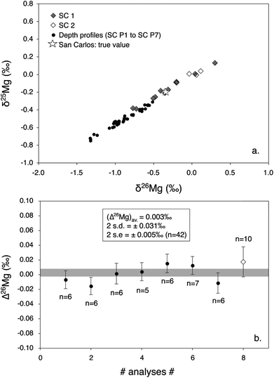Fig. 3 Mg isotopic compositions of San Carlos olivines (Fo#88) measured using two different protocols: either single measurements at different spots (black (SC1) and open (SC2) diamonds, corresponding to two different separated San Carlos olivine grains) or depth profiles (black dots). All data are corrected for matrix effects. The true Mg-isotope composition of San Carlos olivines is also plotted (open star). (a) Three Mg-isotope diagram showing that the two types of data follow the same fractionation law (even if the fractionation is in average stronger for depth profiles). Error bars, typically better than ±0.11‰ on δ²⁵Mg values and ±0.22‰ on δ²⁶Mg values for this analytical session, are not shown for simplicity. (b) Averages of analyses made by depth profiles at different spots (n is the number of analyses in a given depth profile, black dots) compared to the average of the single analyses (n = 10) made at different spots (open diamond). Both types of measurements show Δ²⁶Mg values correctly determined at 0‰ within 2 s.e. Thus, depth profiles can be used in small samples to obtain a precision on Δ²⁶Mg values similar to that obtained from averaging several analyses made at different locations.

Table 2 Mg isotopic compositions of olivines from the San Carlos terrestrial reference material (Fo#88)

Name	Description	δ ^25Mg (‰)	2 s.e	δ ^26Mg (‰)	2 s.e	Δ ^26Mg (‰)	2 s.e	n
SC 1	Separated grain	−0.180	0.103	−0.343	0.206	0.017	0.020	10
SC 2	Separated grain	−0.058	0.059	−0.118	0.126	−0.006	0.023	7
Average						0.007	0.015	17
SC P1	Separated grain – profile no. 1	−0.514	0.029	−0.912	0.067	−0.007	0.012	6
SC P2	Separated grain – profile no. 2	−0.522	0.032	−0.939	0.078	−0.015	0.012	6
SC P3	Separated grain – profile no. 3	−0.493	0.049	−0.862	0.092	0.002	0.014	6
SC P4	Separated grain – profile no. 4	−0.346	0.025	−0.582	0.043	0.004	0.012	5
SC P5	Separated grain – profile no. 5	−0.379	0.024	−0.631	0.035	0.015	0.013	6
SC P6	Separated grain – profile no. 6	−0.552	0.026	−0.969	0.048	0.013	0.012	7
SC P7	Separated grain – profile no. 7	−0.694	0.042	−1.263	0.079	−0.011	0.014	6
Average						0.003	0.005	42
Average						0.002	0.009

---

3.6 Precision reached for the determination of ²⁶Mg excess or deficit

Fig. 4 shows typical results of Δ²⁶Mg measurements for two international and one in-house standards run during one analytical session. The standards show no significant excess or deficit in ²⁶Mg, consistent with their terrestrial origin. The external reproducibility is better than ±0.04‰ (2 s.d., n = 23) and the 2σ error on the mean of all analyses of standards is ±0.018‰ (2 s.e., n = 23).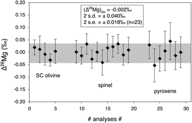

Fig. 4 ²⁶Mg excess or deficit (expressed with the Δ²⁶Mg notation, see text) obtained for three reference materials with different chemical compositions (the same as in Fig. 2) measured within one analytical session (n = 23). They show no significant excess or deficit in ²⁶Mg, consistent with their terrestrial origin. The typical external reproducibility (2 s.d.) is better than ±0.04‰ while the 2σ error of each individual measurement is typically better than ±0.06‰. The 2σ error on the mean of all analyses of reference materials (2 s.e.) is better than ±0.02‰.

The major source of errors on Δ²⁶Mg values that can be identified in the procedure described here, if an improper treatment of the data is performed, is the correction for instrumental fractionation. Because the instrumental fractionation law is always slightly different from the cosmochemical mass fractionation law and from the terrestrial mass fractionation law, an over-correction or an under-correction of instrumental fractionation (due to a poor calibration of matrix effects) will result in an error on Δ²⁶Mg value (Fig. 5). For instance, correcting for an improper Fo content (e.g. Fo#100 instead of Fo#88 for San Carlos olivines) leads to an absolute error on Δ²⁶Mg value of ∼±5 ppm. Similarly, using an improper β value (e.g. β_met instead of β_Earth for San Carlos olivines) can lead to a maximum absolute error of ∼±30 ppm on Δ²⁶Mg (Fig. 5 and Table 3).

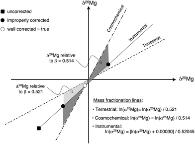Fig. 5 Schematic effect in a three Mg isotope diagram of an improper correction for instrumental isotopic fractionation on the determination of the Δ²⁶Mg value of meteoritic samples. The open dot stands for the isotopic composition after appropriate corrections (see text). In this example no ²⁶Mg excess is obtained since the open dot is sitting on the cosmochemical fractionation line (see text). The two black dots represent wrong corrections of instrumental fractionation in which the matrix effect was under- or over-estimated: this results in “wrong” apparent ²⁶Mg excess or deficit relative to the cosmochemical line (dark grey field). Using erroneously the terrestrial line instead of the cosmochemical line also results in “wrong” ²⁶Mg excess or deficit (light grey field).

Table 3 Effect on the instrumental fractionation of an improper matrix effect correction on San Carlos olivines (Fo#88). The use of an improper Fo content and/or an improper β (β_Earth or β_met) value both impacts upon the final Δ²⁶Mg value (see text). The 2 s.e. on Δ²⁶Mg values is ±0.024‰ whatever the case. Fo# = MgO/(FeO + MgO) (wt%/wt%)

	δ ^25Mg (‰)	Δ ^26Mg (‰)
		β Earth = 0.521	β met = 0.514
Fo#79	−0.997	−0.010	0.016
Fo#88	−0.058	−0.006	−0.004
Fo#100	1.199	−0.001	−0.031

---

3.7 Al and Mg relative ion yields

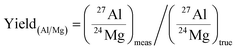
When the ²⁶Mg excesses in meteoritic samples are presumed to be due to the in situ decay of short-lived ²⁶Al, isochron diagrams are built to determine the ²⁶Al/²⁷Al ratio at the time of isotopic closure. For that, the ²⁷Al/²⁴Mg ratios must be determined very precisely in order to minimize the error on the ²⁶Al/²⁷Al (e.g. an error of ±1.3% (see below) in a CAI with ²⁶Al/²⁷Al = 5 × 10⁻⁵ introduces an error of ∼±1.3% on the ²⁶Al/²⁷Al ratio). Because elemental secondary ion yields show strong differences between different elements (and different matrices) that cannot be predicted precisely enough from theoretical grounds,³⁸ they must be calibrated precisely using a set of standards that covers the chemical variability of the samples to analyze.

The Al/Mg relative yield is defined by the ratio between the measured and the true Al/Mg (or ²⁷Al/²⁴Mg) ratios:

Thus the Al/Mg yield is determined from analyses of international and in-house standards and can then be used to correct measurements of samples. Results of the calibration of the Al/Mg yield for various silicates and oxides are then shown in Table 1. Note that all silicates show (for this analytical session) an averaged Al/Mg yield of 0.77 (±0.05, 2 s.d.) with an associated 2 s.e. of 1.3% (n = 28), while oxides such as hibonites show significantly different yields (0.629 (±0.001, 1 s.e.) in this session). Minerals that contain trace amounts of Al, such as olivine, show the same Al/Mg yield as Al-rich silicates within the error (1.00 (±0.30, 1 s.e.) for olivine from the Eagle Station pallasite, having a Al₂O₃ content of ∼0.0027 wt%).

The 2σ error on the ²⁷Al/²⁴Mg ratio is calculated for an individual measurement by summing in a quadratic way the counting error (typically ±2% (2 s.e.) relative in an olivine and ±0.2% (2 s.e.) in a mineral like spinel where Al and Mg are major elements) and the two sigma external reproducibility on the standards (typically ±8% (2 s.e.) in an olivine and ± 1.2% (2 s.e.) in an Al-rich mineral).

4 Examples of the implications of high precision Mg isotopic analyses of components of chondritic meteorites

Using this method, the construction of high precision ²⁶Al isochrons for chondrules and CAIs is within the reach of in situ analysis using ion microprobes. Both the slope (from which the initial (²⁶Al/²⁷Al)₀ ratio is deduced) and the (δ²⁶Mg*)₀ intercept (this notation standing for ²⁶Mg excesses or deficits linked to ²⁶Al in situ decay) can be precisely determined. This gives theoretically access to the crystallization age (calculated from the (²⁶Al/²⁷Al)₀ ratio), and to the ²⁶Al model age of the precursors (calculated from the (δ²⁶Mg*)₀ value with an appropriate evolution model).

Fig. 6 shows as an example of two ²⁶Al isochrons measured for one CAI from the Efremovka CV3 carbonaceous chondrite (data from Mishra and Chaussidon³⁹) and for one chondrule from the Semarkona LL3 ordinary chondrite.⁸ The CAI isochron has a (²⁶Al/²⁷Al)₀ of 4.76 (±0.15) × 10⁻⁵ and a (δ²⁶Mg*)₀ of 0.146 (±0.041)‰, while the chondrule isochron has a (²⁶Al/²⁷Al)₀ of 8.92 (±0.91) × 10⁻⁶ and a (δ²⁶Mg*)₀ of −0.0024 (±0.0075)‰. If interpreted in a simple model considering that there was a time zero when the inner accretion disk was homogenized to (²⁶Al/²⁷Al)_i = 5.23 × 10⁻⁵ and (δ²⁶Mg*)_i = −0.038‰,^5,6,8 the two isochrons imply that the last melting/crystallization event for the CAI and the chondrule took place 0.10^+0.03_−0.03 Myr and 1.86^+0.11_−0.10 Myr, respectively, after the time zero. A 1.2 to 4 Myr age difference between CAIs and chondrules is a general conclusion of ²⁶Al studies interpreted under the assumption of an homogeneous distribution of ²⁶Al in the inner solar system,⁸ which would be consistent with the latest accretion models considering progressive gravitational collapse of mm sized particles concentrated by turbulence in the nebular gas (see review by Dauphas and Chaussidon⁴⁰).

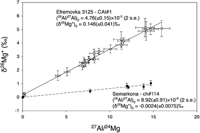Fig. 6 Two ²⁶Al isochrons measured for one CAI from the Efremovka CV3 carbonaceous chondrite (MSWD = 1.15, data from Mishra and Chaussidon, 2012) and for one chondrule from the Semarkona LL3 ordinary chondrite (MSWD = 0.71, data from Villeneuve et al., 2009). A gap ranging from 1.2 to 4 Myr between the ²⁶Al ages of CAIs and chondrules is generally deduced from ²⁶Al studies assuming a homogeneous distribution of ²⁶Al and Mg isotopes in the accretion disk.

The different (δ²⁶Mg*)₀ observed for the CAI and the chondrule can be understood as reflecting different origins and histories for their precursors. The simplest model would be for the chondrule that the precursors were condensed from the nebular gas at 1.86 Myr (age given by the (²⁶Al/²⁷Al)₀ of the chondrule isochron): ²⁶Al decay in the nebular gas with a ²⁷Al/²⁴Mg of 0.101 for 1.86 Myr would result in a δ²⁶Mg* of −0.007‰. For the CAI, the simplest model is that its precursors were condensed at time zero and then evolved in a closed system with the bulk ²⁷Al/²⁴Mg ratio of the CAI of 6.3, leading to the build up of a δ²⁶Mg* of 0.146‰ in 0.10 Myr. However more complicated scenarios are possible^13,35 depending on the model considered.

High precision Mg-isotope measurements are also possible for Mg-rich and Al-poor phases (i.e. phases with a low Al/Mg ratio). This is the case for Mg-rich refractory olivines (either isolated olivines or olivines in porphyritic type I chondrules), whose ²⁶Al model ages could be constrained. These Mg-rich olivines may have various origins. Because they are virtually devoid of Al no radiogenic in-growth of ²⁶Mg takes place, so that their Mg isotopic composition will reflect that of their source, i.e. the nebular gas from which they condensed, the chondrule melt from which they crystallized,^41–43 or the planetesimal mantle from which they crystallized.^44–48 For a given model, the precision on the ²⁶Al model age calculations of these Mg-rich refractory olivines is highly dependent on the precision on both the Δ²⁶Mg value and the ²⁷Al/²⁴Mg ratio. For instance for a parent melt with a ²⁷Al/²⁴Mg ratio of 2.5, a precision of ±0.016‰ on Δ²⁶Mg leads to a precision on the age of ±0.02 Ma (data from Luu et al.⁴⁹).

5 Conclusion

The analytical protocol and data reduction process described in this study allow high precision to be reached for Mg isotopic measurements (²⁵Mg/²⁴Mg and ²⁶Mg/²⁴Mg ratios, as well as ²⁶Mg excess) by MC-SIMS. This method minimizes analytical bias on the final Mg-isotope results, which is very important at the level of precision targeted in cosmochemistry (better than 10 ppm absolute error on the calculation of the final ²⁶Mg excess or deficit).

This new possibility of reaching very high precision for Mg-isotope analyses opens new perspectives in geo- and cosmochemistry fields. For instance natural processes such as biomineralization could be better understood by more accurately constraining the induced fractionation.

Acknowledgements

The authors want to thank Laurent Tissandier for providing the Bacati glass. This work was supported by grant from European Research Council (ERC grant FP7/2007–2013 Grant Agreement no. [226846] Cosmochemical Exploration of the first two Million Years of the Solar System—CEMYSS). This is CRPG-CNRS contribution n°2206.

References

1. A. Bouvier and M. Wadhwa, Nat. Geosci., 2010, 3, 637–641.
2. Y. Amelin, A. N. Krot, I. D. Hutcheon and A. A. Ulyano, Science, 2002, 297, 1678–1683.
3. J. Connelly, Y. Amelin, A. N. Krot and M. Bizzarro, Astrophys. J., 2008, 675, L121–L124.
4. T. Lee, D. A. Papanastassiou and G. J. Wasserburg, Geophys. Res. Lett., 1976, 3, 109–112.
5. K. Thrane, M. Bizzarro and J. A. Baker, Astrophys. J., 2006, 646, L159–L162.
6. B. Jacobsen, Q. Z. Yin, F. Moynier, Y. Amelin, A. N. Krot, K. Nagashima, I. D. Hutcheon and H. Palme, Earth Planet. Sci. Lett., 2008, 272, 353–364.
7. K. Lodders, Astrophys. J., 2003, 591, 1220–1247.
8. J. Villeneuve, M. Chaussidon and G. Libourel, Science, 2009, 325, 985–988.
9. K. K. Larsen, A. Trinquier, C. Paton, M. Schiller, D. Wielandt, M. A. Ivanova, J. N. Connelly, A. Nordlund, A. N. Krot and M. Bizzarro, Astrophys. J., 2011, 735, L37.
10. M. Bizzarro, C. Paton, K. Larsen, M. Schiller, A. Trinquier and D. Ulfbeck, J. Anal. At. Spectrom., 2011, 26, 565–577.
11. J. Villeneuve, M. Chaussidon and G. Libourel, Earth Planet. Sci. Lett., 2011, 301, 107–116.
12. G. J. MacPherson, E. S. Bullock, P. E. Janney, N. T. Kita, T. Ushikubo, A. M. Davis, M. Wadhwa and A. N. Krot, Astrophys. J., 2010, 711, L117–L121.
13. G. J. MacPherson, N. T. Kita, T. Ushikubo, E. S. Bullock and A. M. Davis, Earth Planet. Sci. Lett., 2012, 331–332, 43–54.
14. N. T. Kita and T. Ushikubo, Meteorit. Planet. Sci., 2012, 47, 1108–1119.
15. N. T. Kita, T. Ushikubo, K. B. Knight, R. A. Mendybaev, A. M. Davis, F. M. Richter and J. H. Fournelle, Geochim. Cosmochim. Acta, 2012, 86, 37–51.
16. Secondary Ion Mass Spectrometry: Basic Concepts, Instrumental Aspects, Applications, and Trends, ed. A. Benninghoven, F. G. Rüdenauer and H. W. Werner, Wiley, New York, 1987, p. 1227.
17. E. de Chambost, F. Hillion, B. Rasser and H. N. Migeon, in SIMS VIII Proceedings, ed. A. Benninghoven, K. T. F. Janssen, J. Tumpner and H. W. Werner, New York, John Wiley, 1991, pp. 207–210.
18. E. J. Catanzaro, T. J. Murphy, E. L. Garner and W. R. Shields, J. Res. Natl. Bur. Stand., Sect. A, 1966, 70, 453–458.
19. R. C. Ogliore, G. R. Huss and K. Nagashima, Nucl. Instrum. Methods Phys. Res., Sect. B, 2011, 269, 1910–1918.
20. E. de Chambost, User's Guide for Multicollector Cameca IMS 1270, Cameca, Courbevoie, France, 1997.
21. D. A. Ionov, I. V. Ashchepkov, H.-G. Stosch, G. Witt-Eickschen and H. A. Seck, J. Petrol., 1993, 34, 1141–1175.
22. S. Decitre, PhD thesis, Centre de Recherches Pétrographiques et Géochimiques (CRPG-CNRS), Nancy, 2000.
23. S. Gao, X. Liu, H. Yuan, B. Hattendorf, D. Günther, L. Chen and S. Hu, Geostand. Newsl., 2002, 26, 181–196.
24. W. Yang, F.-Z. Teng and H.-F. Zhang, Earth Planet. Sci. Lett., 2009, 288, 475–482.
25. F.-Z. Teng, W.-Y. Li, S. Ke, B. Marty, N. Dauphas, S. Huang, F.-Y. Wu and A. Pourmand, Geochim. Cosmochim. Acta, 2010, 74, 4150–4166.
26. E. Deloule, C. France-Lanord and F. Albarède, in Stable Isotope Geochemistry: A Tribute to Samuel Epstein, ed. H. P. Taylor, Jr, J. R. O'Neil and I. R. Kaplan, 1991, pp. 53–62.
27. E. D. Young and A. Galy, Rev. Min. Geochem., 2004, 55, 197–230.
28. K. R. Ludwig, ISOPLOT 3: a Geochronological Toolkit for Microsoft Excel, Berkeley Geochronology Centre Special Publication, vol. 4, 2003, p. 74.
29. F. Albarède and B. Beard, Rev. Mineral. Geochem., 2004, 55, 113–152.
30. L. A. Leshin, A. E. Rubin and K. D. McKeegan, Geochim. Cosmochim. Acta, 1997, 61, 835–845.
31. A. Galy, N. S. Belshaw, L. Halicz and R. K. O'Nions, Int. J. Mass Spectrom., 2001, 208, 89–98.
32. E. B. Boulou-Bi, N. Vigier, A. Brenot and A. Poszwa, Geostand. Geoanal. Res., 2009, 33, 95–109.
33. A. Galy, O. Yoffe, P. E. Janney, R. W. Williams, C. Cloquet, O. Alard, L. Halicz, M. Wadhwa, I. D. Hutcheon, E. Ramon and J. Carignan, J. Anal. At. Spectrom., 2003, 18, 1352–1356.
34. E. D. Young, A. Galy and H. Nagahara, Geochim. Cosmochim. Acta, 2002, 66, 1095–1104.
35. A. M. Davis, F. M. Richter, R. A. Mendybaev, P. E. Janney, M. Wadhwa and K. D. McKeegan, 36^th Lunar Planet. Inst. Conf., League City, Texas, 2005.
36. A. M. Davis, A. Hashimoto, R. N. Clayton and T. K. Mayeda, Nature, 1990, 347, 655–658.
37. A. M. Davis and F. M. Richter, in Treatise on Geochemistry, Vol. 1: Meteorites, Planets, and Comets, ed. A. M. Davis, H. D. Holland and K. K. Turekian, Oxford, Elsevier-Pergamon, 2003, pp. 407–430.
38. R. W. Hinton, Chem. Geol., 1990, 83, 11–25.
39. R. K. Mishra and M. Chaussidon, 43^rd Lunar Planet. Sc. Conf., Texas, 2012.
40. N. Dauphas and M. Chaussidon, Annu. Rev. Earth Planet. Sci., 2011, 39, 351–386.
41. N. G. Rudraswami, T. Ushikubo, D. Nakashima and N. T. Kita, Geochim. Cosmochim. Acta, 2011, 75, 7596–7611.
42. H. Nagahara, Nature, 1981, 292, 135–136.
43. R. H. Jones, in International Conference: Chondrules and the Protoplanetary Disk, ed. R. H. Hewins, R. H. Jones and E. R. D. Scott, Cambridge University Press, 1996, pp. 163–172.
44. L. Tissandier, G. Libourel and F. Robert, Meteorit. Planet. Sci., 2002, 37, 1377–1389.
45. G. Libourel, A. N. Krot and L. Tissandier, Earth Planet. Sci. Lett., 2006, 251, 232–240.
46. G. Libourel and A. N. Krot, Earth Planet. Sci. Lett., 2007, 254, 1–8.
47. M. Chaussidon, G. Libourel and A. N. Krot, Geochim. Cosmochim. Acta, 2008, 72, 1924–1938.
48. G. Libourel and M. Chaussidon, Earth Planet. Sci. Lett., 2011, 301, 9–21.
49. T.-H. Luu, M. Chaussidon and J.-L. Birck, 43^rd Lunar Planet. Sc. Conf., Texas, 2012.

---