DOI:
10.1039/C6RA13837C
(Paper)
RSC Adv., 2016,
6, 61516-61527
HKUST-1-MOF–BiVO4 hybrid as a new sonophotocatalyst for simultaneous degradation of disulfine blue and rose bengal dyes: optimization and statistical modelling
Received
27th May 2016
, Accepted 30th May 2016
First published on 8th June 2016
Abstract
A new hybrid material composed of BiVO4 and HKUST-1 MOF (HKUST-1-MOF–BiVO4), which is active under blue light irradiation, was synthesized and characterized by XRD, FE-SEM, BET, BJH, EDS and DRS analysis. Subsequently, this sonophotocatalyst was applied for simultaneous sonophotodegradation of disulfine blue (DB) and rose bengal (RB). The influence of conventional variables such as initial dyes concentration (5–45 mg L−1), HKUST-1-MOF–BiVO4 mass (0.1–0.3 g L−1), flow rate (40–120 mL min−1), pH (2–10) and time of irradiation (5–25 min) upon sonophotocatalytic degradation efficiency was studied by central composite design (CCD). The results analysis revealed that optimum values for the variables studies were found to be 0.2 g L−1, 30 and 30 mg L−1, 80 mL min−1, 6 and 20 min for the HKUST-1-MOF–BiVO4 mass, initial concentration of DB and RB, flow rate, pH and irradiation time, respectively. Under the optimum conditions, the sonophotocatalytic DB and RB degradation percentages at desirability function value of 1.0 were found to be 99.98% and 98.76%, respectively. A kinetics study revealed that the Langmuir–Hinshelwood (L–H) kinetics model was well fitted to the experimental data. Finally, contributions from sonocatalysis and photocatalysis using synergy index and the stability of HKUST-1-MOF–BiVO4 were investigated.
1. Introduction
Arrival of different wastewater of antibiotics, pesticides, synthetic dyes and textiles industries, which contaminated with various pollutant to aquatic ecosystem is associated with hazard and problem for most organism.1 The traditional and most popular pollutants are classified as dyes and metal ions, which among most toxicity emerge from the presence of synthetic dyes and heavy metal ions.2 The presence of positive charge pollutants generally causes more hazards for living things, which has encouraged researchers to apply conventional methods such as adsorption, flocculation, coagulation, biological treatment and membrane processes for separation or transfer to another phase; however, their failure for complete removal or decomposition of these pollutants creates new limitations such as secondary wastes that are expensive to treat and require a secondary separation process.3,4 These limitations were overcome by using advance oxidation processes (AOPs) that benefit from the presence of oxidizing agents (O3, H2O2), radiation (ultraviolet, visible, ultrasound), and catalysts (TiO2, ZnO) which this combination lead to formation of hydroxyl and peroxide radicals as more powerful oxidants in comparison to O3 or H2O2.5,6 Among all the AOPs techniques, sonophotocatalytic degradation processes, which is based on acceleration of photocatalytic efficiency in the presence of a sonophotocatalyst, demonstrate the most advantages compared to the above mention techniques.7,8 In this technique, cavitation generated by ultrasonic waves leads to more immersion of the sonophotocatalyst in the bulk solution, which is increases in surface available area and levering mass transfer resistance ;9–12 after the clean-up procedure, the catalyst surface was regenerated by acoustic microstreaming.13 In this regard, the sonochemically produced H2O2 could be converted into OH radicals during the photolysis process14 and lead to an increased mineralization rate for organic pollutants and more free OH and O2 radicals are available (from photocatalysis and sonolysis).15 In addition, these supplementary radicals are generated by the electron–hole couples created by excitation of the catalyst with light radiation.16–19 The sonophotocatalytic process, despite being a photodegradation procedure based on UV irradiation, is highly recommended in term of its advantage of low toxicity and low costs without the requirement of a cooling system.20 Numerous advantages of LEDs compared to UV light sources, such as high photon efficiency, power system stability and low electrical consumption,21–23 encourage the researcher to design sonophotocatalytic degradation in the invisible region, which completely differs from conventional semiconductors such as ZnO, CuO, and TiO2,13,14 which has a large band gap requiring UV irradiation.24–27 The high abundancy of sunlight in most regions is the driving force for a researcher to construct new materials with band gaps in the visible region that has low cost and efficient wastewater treatment procedure. Among these materials, the photocatalytic behavior of Cu-based MOFs has received considerable attention due to their relatively narrow band gap, large specific surface area, high pore volume and high stability.28,29 It is known that a semiconducting photocatalyst with a narrow band gap is excited under visible light irradiation following the electron (e−) transfer from the valance band (VB) to the conduction band (CB).28,30–32 HKUST-1 MOF as a Cu-based MOFs highly was applied for degradation of organic compounds under visible light irradiation due to its narrow 2.63 eV band gap.33–36 In this regard, Bi-based compounds attracted considerable attention as a photocatalyst due to their narrow band gap, which possibly allows for more activity of these photocatalysts for degradation based on visible-light absorption. Because of the lone pair Bi3+ electrons, the Bi-based compounds were often found to possess hybridized band structures.33 The hybridized states of band structures lead to a reduction of effective mass of holes and electrons and longer residence time and favour a longer traveling distance for excited carriers. All these facts effectively decrease the band gap and increase the light absorption in the long wavelength region, and both phenomena lead to improvement in their photocatalytic activities.34,35 Bismuth-based photocatalysts with the ability to crystallize in different structure types, including Bi2S3, Bi2S3/Bi2WO6, Bi2O3, Bi2O2CO3 and BiVO4, and all forms exhibit high efficiency for organic pollutants degradation.33,36 The combination of Bi3+ and VO43−, due to a unique role of V, for increasing the carrier lifetime and preventing recombination of the electron–hole pairs lead to extension of the absorption range.37,38 Therefore, bismuth vanadate (BiVO4) with an approximate band gap of around 2.4 eV is known as a good and appropriate photocatalyst for the photodegradation process of various pollutants under visible light irradiation.39,40 Therefore, this study is focused on the synthesis of a new hybrid material composed of BiVO4 and HKUST-1 MOF (HKUST-1-MOF–BiVO4), which is active under blue light irradiation for simultaneous sonophotocatalytic degradation of binary mixture of disulfine blue (DB) and rose bengal (RB) dyes. The Langmuir–Hinshelwood (L–H) kinetics model was used for a kinetics study of the sonophotocatalytic degradation process.
2. Experimental
2.1. Materials and apparatus
All reagents and chemicals, including Cu(NO3)2·3H2O, Bi(NO3)3·5H2O, NH4VO3 and HNO3, with the highest purify available were purchased from Merck Company (Darmstadt, Germany). Benzene-1,3,5-tricarboxylicacid disulfine blue and rose bengal were purchased from Sigma Aldrich Company. The spectrum of solutions was obtained by UV-vis spectrophotometry (model V-530, Jasco, Japan). The pH was measured using a pH/redox/temperature meter model AL20 pH (AQUALYTIC, Germany). X-ray diffraction (XRD, Philips PW 1800) was recorded using Cu kα radiation (40 kV and 40 mA). The morphology of samples was analyzed using field emission scanning electron microscopy (FE-SEM: Sigma, Zeiss) and EDS analysis was conducted by a silicon drift detector from Oxford Instruments. Diffuse reflectance spectra (DRS) were obtained with an Avant's spectrophotometer (Avaspec-2048-TEC). The surface area of the material was determined using nitrogen physisorption isotherms on a Micrometrics ASAP 2020 apparatus. Surface area was calculated using the Brunauer–Emmett–Teller (BET) method, and the pore size distribution was obtained from the desorption branch of nitrogen isotherms by means of the Barrett–Joyner–Halenda (BJH) model.
2.2. Synthesis of HKUST-1 MOF, BiVO4 and HKUST-1-MOF–BiVO4 composite
HKUST-1 MOF was prepared by an ultrasound-assisted solvothermal method as follows: benzene-1,3,5-tricarboxylicacid (3.6 mmol) and copper(II) nitrate hemipentahydrate (10 mmol) were sonicated for 1.0 h in 100 mL of solvent consisting 80 mL DMF and 20 mL ethanol in a glass jar. Subsequently, the mixture was transferred into a Teflon-lined autoclave, sealed and heated at 140 °C for 24 h to yield octahedral crystals. Finally, the solvent was removed and heated in an oven at 100 °C for 12 h to yield a porous material. The HKUST-1-MOF–BiVO4 hybrid photocatalysts were prepared via an ultrasound-assisted hydrothermal process as follows: initially, 0.25 g of HKUST-1 MOF was well dispersed in water; subsequently, 2.0 mmol Bi(NO3)3·5H2O and NH4VO3 dissolved in 20 mL HNO3 solution (2 M) were added to the abovementioned solution followed by sonication for 1.0 h at room temperature. The pH value of the aqueous mixture was adjusted with NH4OH solution to 7.0. After sonication for another 30 min at room temperature, the mixture was sealed in a Teflon-lined autoclave and allowed to be heated for the requested durations at a 180 °C hydrothermal temperature under autogenous pressure. Then, the precipitate was washed three times with ethanol and distilled water, and dried at 60 °C for 12 h. For comparison, BiVO4 nanoparticles were also prepared as a blank in parallel but without adding HKUST-1-MOF.
2.3. Experimental set-up and apparatus
The sonophotocatalytic system was a continuous flow-loop, which consisted of a cylindrical reactor, an ultrasonic bath (frequency 25 kHz), a peristaltic pump, an aeration pump, a blue LED, a stirrer, a tank and a sampling valve (Fig. 1). The reactor was a cylindrical glass vessel of 10 cm height and 2.5 and 5 cm inlet and outlet diameter, respectively. The stipe flexible LED first envelopes around a cylindrical pipe and then placed inside the reactor symmetrically. The aeration pump was used to supply demand oxygen and for solution mixing. The peristaltic pump had a control system for solution transfer at certain flow rates. The magnetic stirrer prevented the probable sedimentation of photocatalyst particles. The ultrasonic bath was operated at a fixed 25 kHz frequency. The tank was fed with a 500 mL solution including a binary mixture of dyes and photocatalyst according to the experiment design. All parts of the system were covered with an aluminium foil to avoid light dispersion.
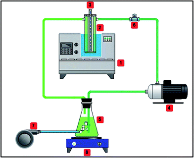 |
| | Fig. 1 Schematic of sonophotocatalytic reactor, (1) ultrasonic bath, (2) reactor vessel, (3) stripe blue LED, (4) peristaltic pump, (5) tank, (6) sampling valve, (7) aeration pump, (8) magnet stirrer. | |
2.4. Sonophotochemical procedure
According to experiment design for each run, a certain amount of BiVO4–HKUST-1 was added to a binary mixture of the dye aqueous solution with calculated initial concentration and well mixed. The solution pH was adjusted to the desired value by 0.1 M HCl and/or NaOH solutions. Then, solution was transferred into the reactor vessel using the peristaltic pump at a certain flow rate. Before switching on the LED, the reactor was operated for 10 min in the dark until reaching the adsorption–desorption equilibrium. During the experiments, the ultrasonic bath temperature was maintained at 25 °C. The sonophotocatalytic degradation efficiency was calculated as follows:| |
 | (1) |
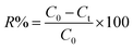
where R is the sonophotocatalytic degradation efficiency (%), and C0 (mg L−1) and Ct (mg L−1) are the initial and residual concentrations of dyes in solution, respectively. Typical UV-vis absorption spectral changes during the sonophotocatalytic degradation are shown in Fig. 2. In each run, with specific conditions, the sample was withdrawn followed by separate phase separation to remove the BiVO4–HKUST-1 particles, and not degraded dyes was calculated according to the solution absorbance and according to respective calibration curve obtained by UV-vis spectrophotometry.
 |
| | Fig. 2 . Typical absorption spectra of RB and DB dyes before and after sonophotodegradation (at different irradiation times). | |
2.5. Experimental design
Central composite design (CCD) based on a statistical model was applied to minimize the number of experiments and indeterminate error and omit systematic error as well as to save time and costs.41–43 Optimization of the process and investigation of the single and combined effect of operational parameters on the process efficiency were determined using response surface methodology (RSM). Statistical modelling of the underlying sonophotocatalytic degradation process to independent parameters (Table 1) viz. initial DB (X1) and RB concentration (X2), pH (X3), HKUST-1-MOF–BiVO4 dosage (X4), flow rate (X5) and irradiation time (X6) was undertaken by small CCD composed of 33 experiments (Table 2) and in all cases, the response was sonophotocatalytic degradation efficiency:44–46
Table 1 Levels of factors in CCD
| Factors |
Levels |
| Low (−1) |
Central (0) |
High (+1) |
−α |
+α |
| X1: DB concentration (mg L−1) |
15 |
25 |
35 |
5 |
45 |
| X2: RB concentration (mg L−1) |
15 |
25 |
35 |
5 |
45 |
| X3: pH |
4 |
6 |
8 |
2 |
10 |
| X4: photocatalyst dosage (g L−1) |
0.15 |
0.20 |
0.25 |
0.10 |
0.30 |
| X5: flow rate (mL min−1) |
60 |
80 |
100 |
40 |
120 |
| X6: time (min) |
10 |
15 |
20 |
5 |
25 |
Table 2 CCD matrix and responses
| Run |
Block |
X1 |
X2 |
X3 |
X4 |
X5 |
X6 |
R1 |
R2 |
| 1 |
1 |
25 |
25 |
2 |
0.20 |
80 |
15 |
72.61 ± 1.2 |
76.40 ± 1.7 |
| 2 |
1 |
15 |
15 |
8 |
0.15 |
60 |
20 |
79.61 ± 1.6 |
82.45 ± 3.2 |
| 3 |
1 |
25 |
25 |
6 |
0.20 |
80 |
15 |
98.30 ± 2.1 |
98.83 ± 2.1 |
| 4 |
1 |
25 |
25 |
6 |
0.20 |
80 |
15 |
98.36 ± 2.3 |
98.84 ± 1.2 |
| 5 |
1 |
25 |
25 |
6 |
0.20 |
80 |
25 |
86.58 ± 2.2 |
88.25 ± 3.1 |
| 6 |
1 |
25 |
25 |
10 |
0.20 |
80 |
15 |
74.58 ± 1.8 |
78.22 ± 1.5 |
| 7 |
1 |
25 |
25 |
6 |
0.20 |
80 |
15 |
98.29 ± 1.9 |
98.81 ± 1.0 |
| 8 |
1 |
35 |
35 |
8 |
0.25 |
60 |
10 |
60.02 ± 1.8 |
61.43 ± 1.0 |
| 9 |
1 |
25 |
25 |
6 |
0.30 |
80 |
15 |
76.08 ± 1.4 |
79.21 ± 1.2 |
| 10 |
1 |
35 |
15 |
4 |
0.15 |
100 |
10 |
41.23 ± 0.7 |
62.86 ± 2.0 |
| 11 |
1 |
25 |
25 |
6 |
0.20 |
80 |
15 |
98.39 ± 3.2 |
98.82 ± 1.6 |
| 12 |
1 |
15 |
15 |
4 |
0.15 |
60 |
10 |
60.22 ± 2.1 |
64.21 ± 1.7 |
| 13 |
1 |
35 |
35 |
8 |
0.15 |
100 |
10 |
41.28 ± 1.0 |
44.87 ± 1.3 |
| 14 |
1 |
15 |
35 |
4 |
0.25 |
100 |
20 |
81.45 ± 2.0 |
64.29 ± 1.1 |
| 15 |
1 |
45 |
25 |
6 |
0.20 |
80 |
15 |
75.27 ± 1.2 |
87.71 ± 1.9 |
| 16 |
1 |
35 |
15 |
4 |
0.25 |
60 |
10 |
40.15 ± 1.4 |
64.93 ± 1.4 |
| 17 |
1 |
25 |
5 |
6 |
0.20 |
80 |
15 |
87.17 ± 1.5 |
88.94 ± 1.2 |
| 18 |
1 |
15 |
35 |
4 |
0.15 |
60 |
20 |
80.46 ± 1.5 |
64.45 ± 1.7 |
| 19 |
1 |
25 |
25 |
6 |
0.10 |
80 |
15 |
66.52 ± 1.6 |
69.44 ± 2.3 |
| 20 |
1 |
25 |
45 |
6 |
0.20 |
80 |
15 |
88.23 ± 1.1 |
77.66 ± 1.2 |
| 21 |
1 |
25 |
25 |
6 |
0.20 |
40 |
15 |
72.71 ± 2.2 |
76.08 ± 0.9 |
| 22 |
1 |
35 |
15 |
8 |
0.25 |
60 |
20 |
60.14 ± 1.4 |
83.89 ± 2.1 |
| 23 |
1 |
15 |
15 |
8 |
0.25 |
100 |
20 |
81.79 ± 1.2 |
84.34 ± 2.3 |
| 24 |
1 |
25 |
25 |
6 |
0.20 |
80 |
15 |
98.35 ± 2.4 |
98.86 ± 1.2 |
| 25 |
1 |
35 |
35 |
4 |
0.25 |
60 |
20 |
60.51 ± 1.1 |
64.42 ± 2.0 |
| 26 |
1 |
25 |
25 |
6 |
0.20 |
120 |
15 |
74.07 ± 1.9 |
76.34 ± 3.1 |
| 27 |
1 |
35 |
35 |
4 |
0.15 |
100 |
20 |
61.27 ± 1.8 |
64.42 ± 1.0 |
| 28 |
1 |
35 |
15 |
8 |
0.15 |
100 |
20 |
62.52 ± 1.7 |
84.35 ± 1.3 |
| 29 |
1 |
25 |
25 |
6 |
0.20 |
80 |
5 |
28.35 ± 2.2 |
30.91 ± 2.0 |
| 30 |
1 |
15 |
15 |
4 |
0.25 |
100 |
10 |
63.03 ± 2.3 |
65.72 ± 1.9 |
| 31 |
1 |
15 |
35 |
8 |
0.25 |
100 |
10 |
62.36 ± 0.8 |
43.96 ± 1.5 |
| 32 |
1 |
5 |
25 |
6 |
0.20 |
80 |
15 |
89.76 ± 2.5 |
87.37 ± 2.3 |
| 33 |
1 |
15 |
35 |
8 |
0.15 |
60 |
10 |
61.62 ± 2.0 |
41.75 ± 0.9 |
Analysis of Variance (ANOVA) was applied to evaluate model significance according to well-known criteria such as P and F values based on their comparison with respective values are presented in a statistical reference table.47–49
3. Results and discussion
3.1. Characterization of samples
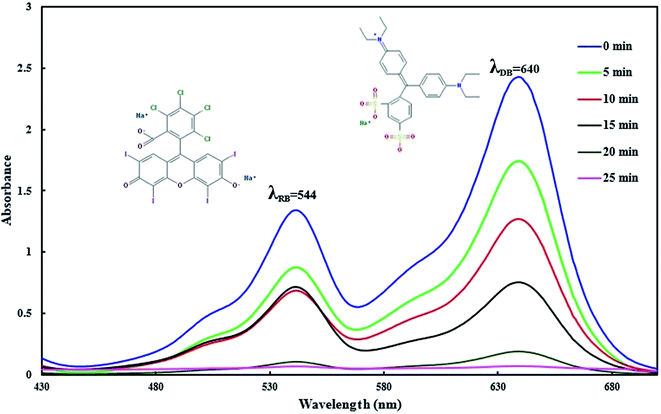
Diffuse reflectance spectra analysis (Fig. 3) was used for calculating the energy band gap of BiVO4–HKUST-1 based on the following equation:where α is the absorption coefficient, A is a proportionality constant and ν is the frequency of photons and Eg is the absorption band gap. Plotting the (αhν)2 versus hν (Fig. 3) at zero intercept showed that the direct band gap for HKKUST-1 and BiVO4–HKUST-1 was 2.63 eV and 1.86 eV, respectively, which strongly prove their ability as a photocatalyst in the presence of blue light.
 |
| | Fig. 3 . DRS of HKUST-1-MOF (a) and HKUST-1–BiVO4 (b) (inset: the plot of (αhν)2 versus hν was used to calculate the samples band gap). | |
The XRD pattern of HKUST-1 MOF (Fig. 4a) is composed of main peaks at 2θ = 5.7°, 9.36°, 11.46°, 13.11°, 14.81°, 16.56°, 17.61°, 19.10°, 20.26°, 23.46°, 24.16°, 26.0° and 29.46°, which corresponds to the (200), (220), (222), (400), (311), (422), (511), (440), (600), (444), (551), (731) and (751) crystal planes of the pure solid phase copper (PDF card no. 04-0836).
 |
| | Fig. 4 XRD pattern of HKUST-1 MOF and HKUST-1–BiVO4. | |
In the XRD BiVO4–HKUST-1 pattern (Fig. 4), all the diffraction peaks at 2θ of 18.01°, 22.26°, 27.71°, 42.5° and 53° are assigned to (020), (011), (121), (150) and (161) can be indexed to a monoclinic BiVO4 (reference code: 00-014-0688). In the XRD pattern of the as-prepared HKUST-1-MOF–BiVO4 heterogeneous nanostructures, the diffraction peaks of HKUST-1-MOF in the 18–65° range due to overlap with BiVO4 peaks cannot be detected (Fig. 4), whereas the other peaks for HKUST-1 (5.7°, 9.36°, 11.46°, 13.11°, 14.81°, 16.56° and 17.61°) are quite obvious. This is possibly attributed to the high crystallinity of the BiVO4 phase, which makes it appear as the dominant peaks in the XRD pattern of the BiVO4–NPs–HKUST-1-MOF heterogeneous nanostructures.
The morphology of the resulting crystals of HKUST-1 MOF and BiVO4–HKUST-1 is shown in the FE-SEM micrographs (Fig. 5), which shows that the approximate size of octahedral HKUST-1 MOF was about 1.0 μm (Fig. 5a). The SEM image of BiVO4–HKUST-1 (Fig. 5b) exhibited a plate-like morphology with a 200–500 nm thickness and demonstrated that the surfaces of BiVO4 nanocrystals were very smooth and clean.
 |
| | Fig. 5 FE-SEM image of HKUST-1 MOF (a) and HKUST-1–BiVO4 (b). | |
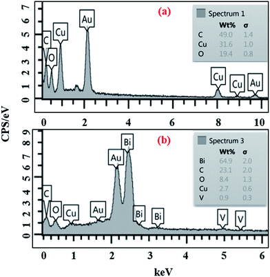
EDS analysis (Fig. 6) revealed that the elemental composition of the obtained HKUST-1 consisted of only C, O and Cu, indicating the high purity of the products (Fig. 6a), while the presence of C, O, Bi, V and Cu showed successful formation of HKUST-1-MOF–BiVO4 (Fig. 6b).
 |
| | Fig. 6 . EDS image of HKUST-1 MOF (a) and HKUST-1–BiVO4 (b). | |
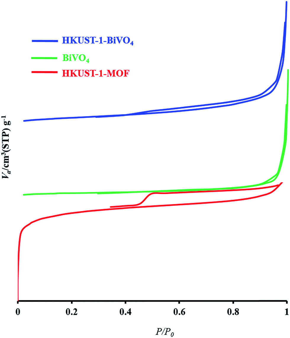
The textural and physicochemical properties of BiVO4 nanoparticles, HKUST-1 MOF and HKUST-1-MOF–BiVO4 composites such as the pore diameter (BJH), the BET surface area and total pore volume (Vtotal), are given in Table 3. HKUST-1 and BiVO4 nitrogen adsorption–desorption measurements indicated 855 and 30 m2 g−1 BET surface areas, respectively. The final 585 m2 g−1 surface area after composite formation was seen (see Fig. 7 and Table 2). The decreased BET surface area, mesoporous volume and average pore diameter after the modification indicated successful composite formation. The high BET surface area, mesoporous volume and average pore diameter of HKUST-1-MOF–BiVO4 means the composite can facilitate the enhanced photocatalytic activity.
Table 3 Textural and physicochemical properties of the samples
| Sample |
BET surface area (m2 g−1) |
Pore diameter (BJH) (nm) |
Total pore volume (m3 g−1) |
| HKUST-1-MOF |
855 |
3.50 |
1.32 |
| BiVO4 |
30 |
1.25 |
0.12 |
| HKUST-1-MOF–BiVO4 |
585 |
2.50 |
1.02 |
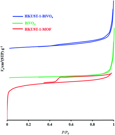 |
| | Fig. 7 Adsorption–desorption isotherm of BiVO4-1, HKUST-1 MOF, and HKUST-1–BiVO4. | |
3.2. Analysis of variance
A quadratic model based on ANOVA analysis was achieved to evaluate the experimental data according to F-values, P-values and lack of fit (Table 4), which used to investigate the model significance (P-values < 0.050 are significant). The non-significant lack-of-fit revealed the good predictability of the quadratic model. ANOVA results revealed a high coefficient of determination, whereas the R-square of model was found to be 0.99 with a high closeness to 1. All parameters and their interaction were significant according to the very small P-values and non-significant lack-of-fit. The final model was fitted with the polynomial equations in terms of coded factors as follows for predicting the photodegradation percentage for DB and RB:| | |
R1 = 98.33 − 3.62X1 + 0.26X2 + 0.49X3 + 2.39X4 + 0.34X5 + 14.56X6 + 1.11X1X2 + 1.29X1X3 + 0.83X1X4 + 1.06X1X5 − 0.90X1X6 + 5.94X2X3 + 1.14X2X4 − 1.54X2X5 − 0.82X2X6 + 1.08X3X4 − 1.19X3X5 − 1.0X3X6 + 5.34X4X5 − 1.32X4X6 + 1.28X5X6 − 3.95X12 − 2.65X22 − 6.18X32 − 6.75X42 − 6.23X52 − 10.21X62
| (3) |
| | |
R2 = 98.83 + 0.085X1 − 2.82X2 + 0.45X3 + 2.44X4 + 0.065X5 + 14.33X6 + 1.34X1X2 + 1.51X1X3 + 0.86X1X4 + 0.97X1X5 − 1.06X1X6 + 5.41X2X3 + 0.85X2X4 − 1.02X2X5 − 0.28X2X6 + 1.05X3X4 − 0.71X3X5 + 6.13X3X6 − 1.17X4X5 − 1.32X4X6 + 1.07X5X6 − 2.82X12 − 3.88X22 − 5.38X32 − 6.13X42 − 5.66X52 − 9.81X62
| (4) |
where R1 and R2 are the sonophotocatalytic degradation percentages of DB and RB, respectively.
Table 4 ANOVA for the quadratic model
| Source of variation |
DFa |
DB |
RB |
| SSb |
MSc |
F-Value |
P-Value |
SSb |
MSc |
F-Value |
P-Value |
| Degree of freedom. Sum of square. Mean of square. |
| Model |
27 |
10![[thin space (1/6-em)]](https://www.rsc.org/images/entities/char_2009.gif) 724.32 724.32 |
397.197 |
191189.90 |
<0.0001 |
9895.98 |
366.52 |
1.20 × 10⁶ |
<0.0001 |
| X1 |
1 |
104.9801 |
104.9801 |
50531.91 |
<0.0001 |
0.058 |
0.058 |
188.48 |
<0.0001 |
| X2 |
1 |
0.5618 |
0.5618 |
270.4212 |
<0.0001 |
63.62 |
63.62 |
2.08 × 10⁵ |
<0.0001 |
| X3 |
1 |
1.94045 |
1.94045 |
934.0313 |
<0.0001 |
1.66 |
1.66 |
5400.65 |
<0.0001 |
| X4 |
1 |
45.6968 |
45.6968 |
21996.05 |
<0.0001 |
47.73 |
47.73 |
1.56 × 10⁵ |
<0.0001 |
| X5 |
1 |
0.9248 |
0.9248 |
445.1504 |
<0.0001 |
0.034 |
0.034 |
110.22 |
0.0001 |
| X6 |
1 |
1695.366 |
1695.366 |
816060.90 |
<0.0001 |
1643.94 |
1643.94 |
5.36 × 10⁶ |
<0.0001 |
| X1X2 |
1 |
19.8025 |
19.8025 |
9531.889 |
<0.0001 |
28.57 |
28.57 |
93159.86 |
<0.0001 |
| X1X3 |
1 |
26.47103 |
26.47103 |
12741.77 |
<0.0001 |
36.24 |
36.24 |
1.18 × 10⁵ |
<0.0001 |
| X1X4 |
1 |
3.652033 |
3.652033 |
1757.898 |
<0.0001 |
3.94 |
3.94 |
12862.61 |
<0.0001 |
| X1X5 |
1 |
6.020833 |
6.020833 |
2898.115 |
<0.0001 |
4.98 |
4.98 |
16237.2 |
<0.0001 |
| X1X6 |
1 |
12.8164 |
12.8164 |
6169.146 |
<0.0001 |
17.85 |
17.85 |
58208.56 |
<0.0001 |
| X2X3 |
1 |
188.3376 |
188.3376 |
90655.90 |
<0.0001 |
155.81 |
155.81 |
5.08 × 10⁵ |
<0.0001 |
| X2X4 |
1 |
20.65703 |
20.65703 |
9943.213 |
<0.0001 |
11.56 |
11.56 |
37695.65 |
<0.0001 |
| X2X5 |
1 |
38.13063 |
38.13063 |
18354.09 |
<0.0001 |
16.61 |
16.61 |
54148.78 |
<0.0001 |
| X2X6 |
1 |
3.597075 |
3.597075 |
1731.444 |
<0.0001 |
0.41 |
0.41 |
1351.33 |
<0.0001 |
| X3X4 |
1 |
18.7489 |
18.7489 |
9024.741 |
<0.0001 |
17.60 |
17.60 |
57384.86 |
<0.0001 |
| X3X5 |
1 |
22.7529 |
22.7529 |
10952.06 |
<0.0001 |
7.95 |
7.95 |
25931.74 |
<0.0001 |
| X3X6 |
1 |
5.360033 |
5.360033 |
2580.04 |
<0.0001 |
200.25 |
200.25 |
6.53 × 10⁵ |
<0.0001 |
| X4X5 |
1 |
152.1544 |
152.1544 |
73239.19 |
<0.0001 |
7.24 |
7.24 |
23603.91 |
<0.0001 |
| X4X6 |
1 |
28.03703 |
28.03703 |
13495.56 |
<0.0001 |
27.77 |
27.77 |
90563.8 |
<0.0001 |
| X5X6 |
1 |
26.06103 |
26.06103 |
12544.42 |
<0.0001 |
18.28 |
18.28 |
59594.43 |
<0.0001 |
| X12 |
1 |
469.8734 |
469.8734 |
226172.50 |
<0.0001 |
240.14 |
240.14 |
7.83 × 10⁵ |
<0.0001 |
| X22 |
1 |
212.0752 |
212.0752 |
102081.90 |
<0.0001 |
454.28 |
454.28 |
1.48 × 10⁶ |
<0.0001 |
| X32 |
1 |
1150.207 |
1150.207 |
553649.60 |
<0.0001 |
872.14 |
872.14 |
2.84 × 10⁶ |
<0.0001 |
| X42 |
1 |
1373.697 |
1373.697 |
661225.90 |
<0.0001 |
1130.8 |
1130.8 |
3.69 × 10⁶ |
<0.0001 |
| X52 |
1 |
1169.364 |
1169.364 |
562870.60 |
<0.0001 |
963.56 |
963.56 |
3.14 × 10⁶ |
<0.0001 |
| X62 |
1 |
3141.029 |
3141.029 |
1511927 |
<0.0001 |
2900.62 |
2900.62 |
9.46 × 10⁶ |
<0.0001 |
| Residual |
5 |
0.010388 |
0.002078 |
|
|
1.53 × 10⁻³ |
3.07 × 10⁻⁴ |
|
|
| Lack of fit |
1 |
0.003308 |
0.003308 |
1.868644 |
0.2434 |
5.33 × 10⁻⁵ |
5.33 × 10⁻⁵ |
0.14 |
0.7235 |
| Pure error |
4 |
0.00708 |
0.00177 |
|
|
1.48 × 10⁻³ |
3.70 × 10⁻⁴ |
|
|
| Cor total |
32 |
10724.33 |
|
|
|
9895.98 |
|
|
|
3.3. Response surface plots
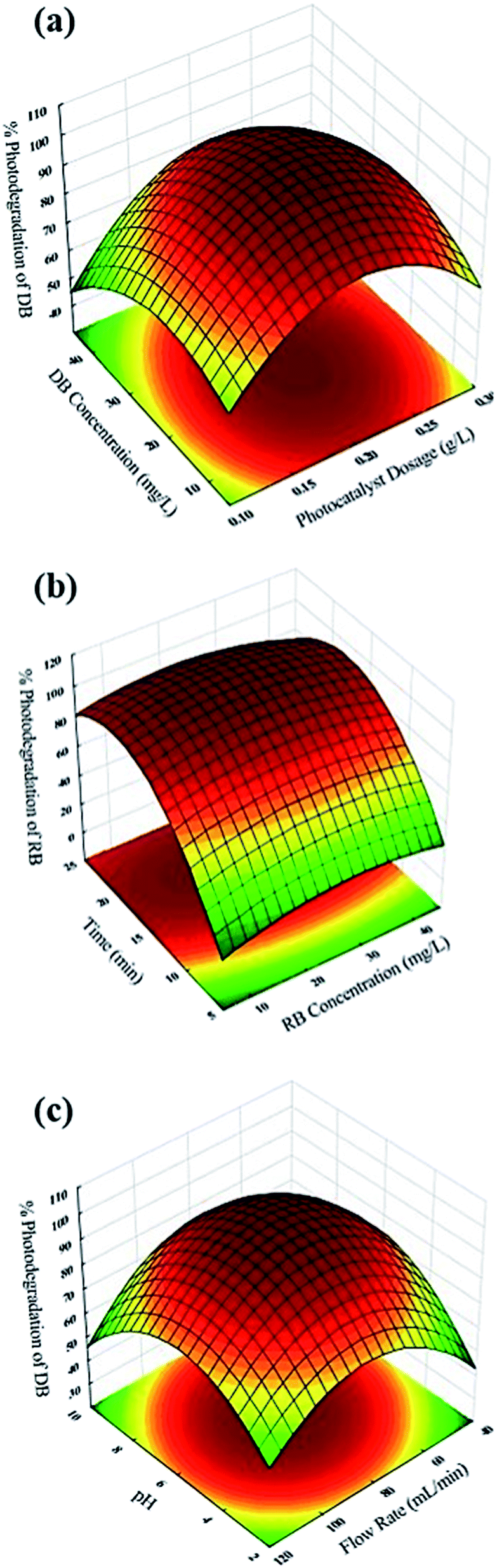
Three dimensional (3D) response surface plots (Fig. 8) show that BiVO4–HKUST-1 mass had a positive effect on process efficiency (Fig. 8a) and therefore increasing its value le to creation of more free radicals, which possibly increased the degradation. Exceeding the photocatalyst mass values higher than 0.2 g L−1 led to creating a dark condition that inhibited light penetration and hence diminished the sonophotocatalytic degradation percentage. Flow rate is an important operational parameter in continuous-flow mode sonophotocatalytic processes and had a positive and negative influence in degradation percentage. Increasing the flow rate up to 80 mL min−1 led to increased efficiency (Fig. 8c). This fact may be related to improved convective mass transfer and contact time of dye molecules with the photocatalyst surface in the reactor. Flow rates below 80 mL min−1 have convective mass transfer as the primary limiting factor for sonophotocatalytic degradation. Increasing the flow rate improved the photocatalytic reaction by enhancing the transfer of dye molecules and oxygen to the photocatalyst surface. Flow rates higher than 80 mL min−1 are associated with decreasing contact time among dyes and photocatalyst, which is proportional to faster photocatalytic reaction.50,51 Illumination time had a positive influence on sonophotocatalytic degradation percentage (Fig. 8b), indicating that higher illumination time leads to more pollutant exposure to the illumination as well as more free radical presence, all of which contribute to improving the sonophotocatalytic degradation efficiency. The effect of initial DB and RB concentration on the sonophotocatalytic degradation percentage revealed that at lower concentration, more degradation percentage was achieved and increased dye concentration was associated with lower sonophotocatalytic degradation efficiency (Fig. 8a and b). Higher dye concentration means a reduction of the number of activated photocatalysts per dye molecule, which leads to a reduction in procedure efficiency, while on the other hand due to the fact that the solution became turbid and the light penetration depth decreased as well as light distribution being insufficient led to fewer activation sites and consequently to less photocatalytic degradation.
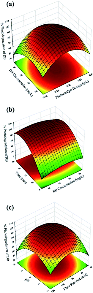 |
| | Fig. 8 Response surfaces plots of central composite design: (a) DB concentration-BiVO4–HKUST-1 dosage; (b) illumination time-RB concentration; (c) pH-flow rate. | |
The pH is an important and effective parameter in sonophotocatalytic degradation of dyes, and in this regard similar experiments with the initial pH in the 2.0–10 range were examined. The response behavior at different pH values (Fig. 8c) shows the maximum photodegradation percentage was achieved at pH 6. This was related to the maximum accumulation of dye molecules on the external surface of neutral photocatalyst and maximum dye photodegradation was observed. On the other hand, at pH > 6.0, OH− ions have a great challenge to reach of dyes molecules on the photocatalyst surface and a diminished response was observed. Therefore, the optimum pH value was 6.0.
3.4. Optimization study
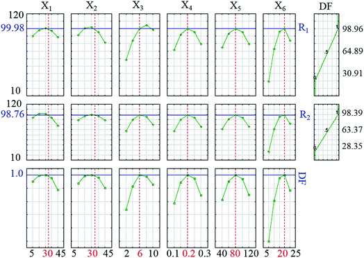
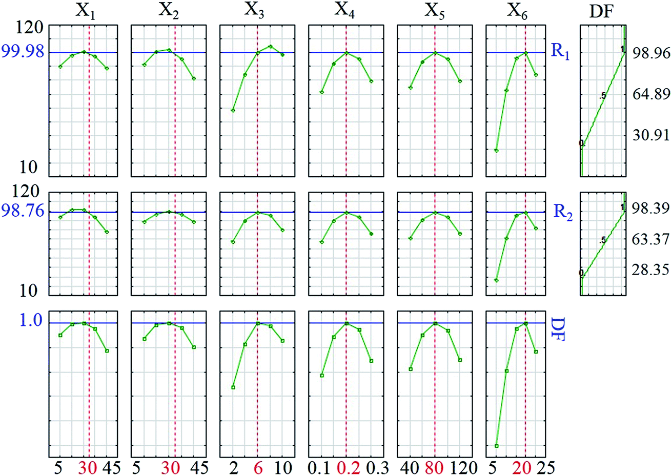
The desirability profile response based on Statistical software (ver. 10.0) was used to assign the optimum values of independent operational parameters to achieve maximum sonophotocatalytic degradation efficiency. The desirability functions vary from 0.0 (undesirable) to 1.0 (very desirable) and according to respective values, which are presented in Fig. 9, the best desirability function was observed at 0.2 g L−1, 30 and 30 mg L−1, 80 mL min−1, 6 and 20 min for the HKUST-1-MOF–BiVO4 mass, initial concentration of DB and RB, flow rate, pH and irradiation time, respectively. Under the optimum conditions, the sonophotocatalytic degradation percentages of DB and RB were found to be 99.98% and 98.76%, respectively, with a 1.0 desirability score.
 |
| | Fig. 9 Profiles of predicated values and desirability function for photodegradation of DB and RB. | |
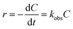
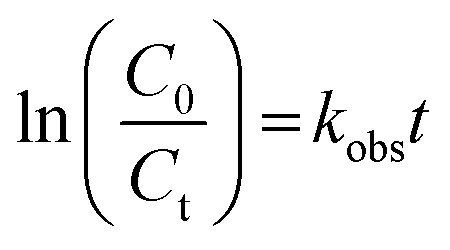
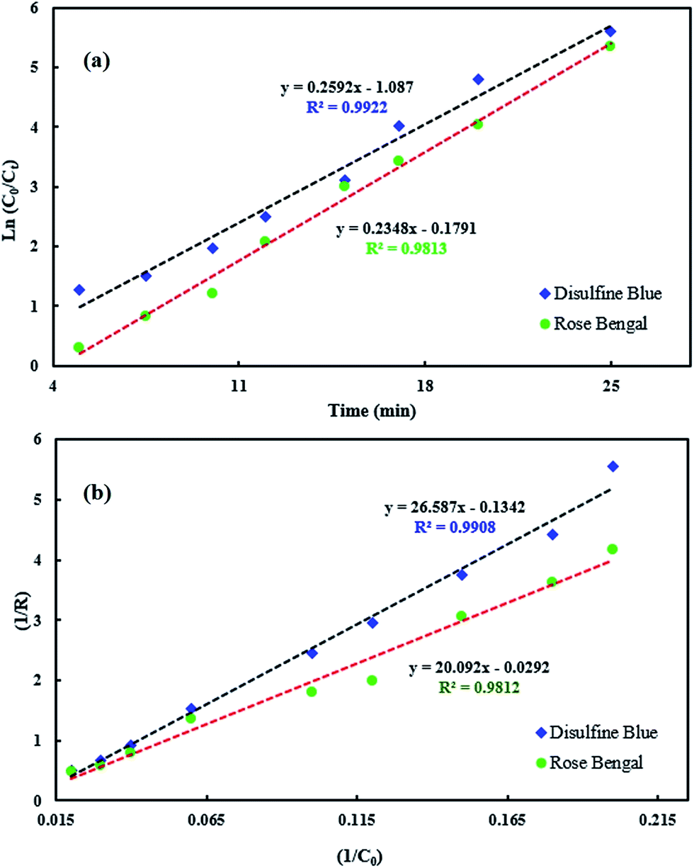
3.5. Kinetics of sonophotocatalytic degradation
The sonophotocatalytic degradation of disulfine blue and rose bengal obeyed the following pseudo first order kinetics based on the Langmuir–Hinshelwood (L–H) model, which is the most common kinetic model for organic and dyes compounds degradation:52–54| |
 | (5) |
where C is the concentration of dye and kobs (min−1) is the observed first-order rate constant. On integrating eqn (5), the following concentration–time equation is achieved:| |
 | (6) |
This linear form was used for fitting the experimental data by plotting ln(C0/Ct) versus irradiation time. The slope of above equation equals the observed first-order rate constant for sonophotocatalytic degradation. Fig. 9 shows that pseudo first order kinetics were well fitted with empirical data for DB and RB sonophotocatalytic degradation.
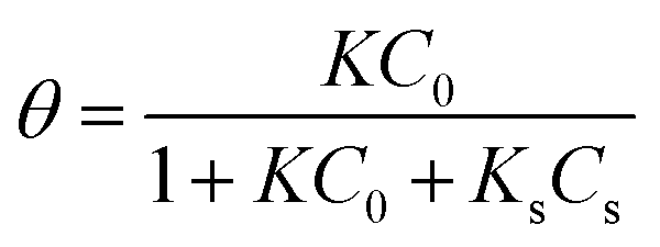
The dye degradation on the BiVO4–HKUST-1 surface can be explained by the Langmuir–Hinshelwood (L–H) kinetic model, which was strongly sufficient for explanation and representation of the reaction occurring at a solid–liquid interface. In this model, the reaction rate is proportional to the surface coverage θ:55
| |
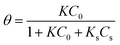 | (7) |
where
K and
Ks are the adsorption coefficient of the substrate (dye) and the solvent;
C0 and
Cs are the initial concentrations of the substrate and solvent.
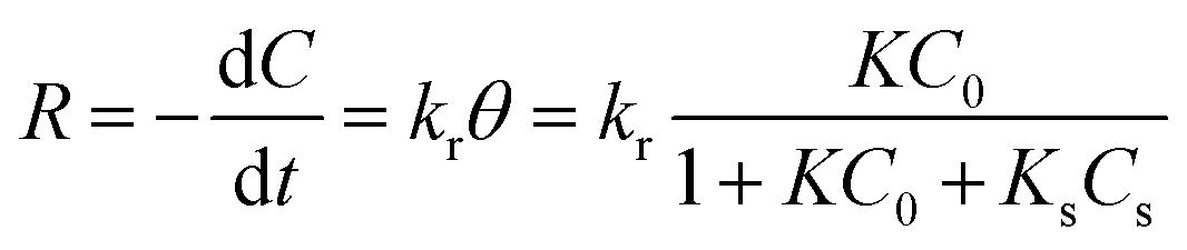
The apparent sonophotocatalytic degradation rate (R) at the catalyst surface can be expressed as a single-component L–H kinetic rate expression as follows:
| |
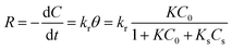 | (8) |
where
kr (mg min
−1 L
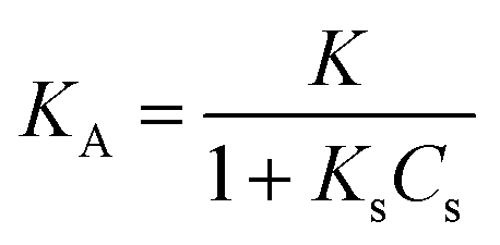
−1) is the apparent sonophotocatalytic degradation rate constant. By definition of
KA (L mg
−1):
| |
 | (9) |
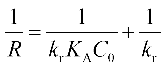
By inserting eqn (9) in (8) and rearranging the following is obtained:
| |
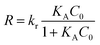 | (10) |
By rearranging eqn (10), the following final equation will be derived:
| |
 | (11) |
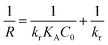
Validation of Langmuir–Hinshelwood model for sonophotocatalytic degradation of DB and RB was evaluated by plotting 1/R versus 1/C0 for each dye. Linear plots show that the L–H model fit the sonophotocatalytic degradation kinetics of the dyes well (Fig. 10).
 |
| | Fig. 10 Plots of the L–H kinetic model. (a) ln(C0/Ct) vs. irradiation time; (b) 1/R vs. 1/C0. | |
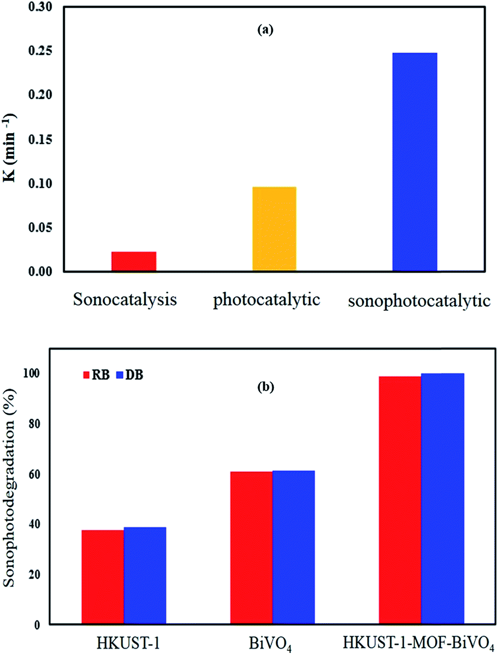
3.6. Synergistic effect
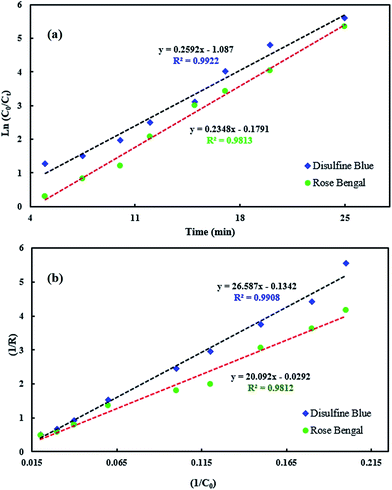
The contributions from sonocatalysis and photocatalytic were investigated using synergy index, which is the ratio of the sonophotocatalytic rate constant to the sum of the rate constants of the individual processes (eqn (12)). This factor also was applied to evaluation of the synergistic effect of the hybrid system, including the sonocatalysis and photocatalytic processes:56,57| |
 | (12) |
where ksonophotocatalytic, ksonocatalytic and kphotocatalytic are the apparent rate constant of sonophotocatalytic, sonocatalysis and photocatalytic processes, respectively. Synergistic effect values greater than 1 show a positive effect. Results for degradation of DB and RB indicated that the combined system had a positive effect on efficiency compared with individual processes (Table 5). Comparing the degradation rates for different processes at the optimum values indicated a contribution of each process on degradation efficiency (Fig. 11), and it was clear that the reaction rate constant of the sonophotocatalytic process was greater than that of the sum of the rate constants of the individual processes, i.e. ksonophoto > kphoto + ksono. The synergetic effect can be attributed to the role of ultrasonic waves to de-aggregating the photocatalyst particles, increasing surface area and catalyst activity as well as increasing in mass transfer. In fact, chemical effects of ultrasonic field due to acoustic cavitation, which is the formation, growth, and collapse of bubbles in liquid, lead to a faster degradation rate and degradation efficiency enhancement.58–60
Table 5 Synergy index for the sonophotocatalytic system and individual processes
| HKUST-1–BiVO4 dosage (g L−1) |
k (min−1) |
Synergy index |
| Sonocatalysis |
Photocatalyst |
Sonophotocatalyst |
| 0.10 |
0.017 |
0.058 |
0.142 |
1.89 |
| 0.15 |
0.019 |
0.077 |
0.193 |
2.01 |
| 0.20 |
0.023 |
0.096 |
0.247 |
2.07 |
| 0.25 |
0.020 |
0.085 |
0.205 |
1.95 |
| 0.30 |
0.019 |
0.082 |
0.166 |
1.64 |
 |
| | Fig. 11 Comparison of degradation rates for different processes (a) and contributions of prepared samples in the sonophotocatalyst process (b). | |
The study of the contributions for BiVO4 and HKUST-1 MOF and their composite at optimum values (Fig. 11b) indicated that contribution of BiVO4 was higher than HKUST-1-MOF but lower than the HKUST-1-MOF–BiVO4 composite, which reveals that the coupling of HKUST-1 and BiVO4 is helpful to separate the photogenerated of DB and RB dyes.
3.7. Stability and reusability of HKUST-1-MOF–BiVO4
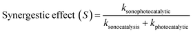
To evaluate the stability and reusability of HKUST-1-MOF–BiVO4, additional experiments were conducted to degrade DB and RB dyes under blue LED light cycled for five times (Fig. 12). After every cycle, the catalyst was washed and heated at 80 °C and assumed to be completely dried and cleaned to conduct the next photodegradation experiment under similar optimized conditions. As seen, the DB and RB dyes were quickly degraded after every injection of the DB and RB solution. The HKUST-1-MOF–BiVO4 was stable under repeated photocatalytic reaction with a nearly constant photodecomposition rate. These results demonstrate that the HKUST-1-MOF–BiVO4 sample is a very stable visible-light photocatalyst due to effective anchoring of HKUST-1-MOF–BiVO4, which would inhibit the leaching of Bi, V, Cu or other compounds into the solution. Therefore, it can be proposed that the HKUST-1-MOF–BiVO4 hybrid is a stable and superior catalyst with enhanced photocatalytic activity.
 |
| | Fig. 12 The cycling sonophotocatalyst degradation efficiency for DB (a) and RB (b) of BiVO4–HKUST-1 under visible-light irradiation. | |
4. Conclusion
Performance of a continuous flow-loop sonophotocatalytic reactor was investigated for simultaneous degradation of Disulfine Blue (DB) and Rose Bengal (RB) as a binary dye mixture. HKUST-1-MOF–BiVO4 as a photocatalyst was synthesized and analysed by XRD, EDS, DRS, BET, BJH and FE-SEM then applied under blue LED irradiation. Design of experiments based on response surface methodology was used to process, model and evaluate the interaction of operational parameters for sonophotocatalytic degradation efficiency. Optimizing independent parameters to achieve maximum degradation efficiency was performed using STATISTICA Software as well as by Desirability Function (DF). The effect of six parameters included the initial DB and RB concentration, pH, flow rate, photocatalyst dosage and irradiation time upon sonophotocatalytic degradation efficiency was studied and the results revealed that optimum values of these parameter for maximum efficiency percentage (99.98% DB and 98.76% RB) are 30 and 30 mg L−1, 6, 80 mL min−1, 0.2 g L−1 and 20 min for initial concentration of DB and RB, pH, flow rate, photocatalyst dosage and irradiation time, respectively. Kinetic study analysis revealed that a pseudo first order model based on Langmuir–Hinshelwood is appropriate for successful fitting of the experimental data. Finally, contributions from sonocatalysis and photocatalytic based on synergy index and stability HKUST-1-MOF–BiVO4 were investigated.
Acknowledgements
The authors thank the Research Council of the Yasouj University and Iran National Science Foundation (Grant No. 94/ /41301) for their financial support.
References
- M. N. Chong, B. Jin, C. W. Chow and C. Saint, Water Res., 2010, 44, 2997–3027 CrossRef CAS PubMed.
- M. Shirzad-Siboni, M. Farrokhi, R. Darvishi Cheshmeh Soltani, A. Khataee and S. Tajassosi, Ind. Eng. Chem. Res., 2014, 53, 1079–1087 CrossRef CAS.
- J. Choina, C. Fischer, G.-U. Flechsig, H. Kosslick, V. Tuan, N. Tuyen, N. Tuyen and A. Schulz, J. Photochem. Photobiol., A, 2014, 274, 108–116 CrossRef CAS.
- M. Dükkancı, M. Vinatoru and T. J. Mason, Ultrason. Sonochem., 2014, 21, 846–853 CrossRef PubMed.
- B. Wols and C. Hofman-Caris, Water Res., 2012, 46, 2815–2827 CrossRef CAS PubMed.
- M. Antonopoulou, E. Evgenidou, D. Lambropoulou and I. Konstantinou, Water Res., 2014, 53, 215–234 CrossRef CAS PubMed.
- P. Sathishkumar, R. V. Mangalaraja, H. D. Mansilla, M. Gracia-Pinilla and S. Anandan, Appl. Catal., B, 2014, 160, 692–700 CrossRef.
- C. L. Bahena, S. S. Martínez, D. M. Guzmán and M. D. R. T. Hernández, Chemosphere, 2008, 71, 982–989 CrossRef CAS PubMed.
- F. N. Azad, M. Ghaedi, K. Dashtian, S. Hajati and V. Pezeshkpour, Ultrason. Sonochem., 2016, 31, 383–393 CrossRef CAS PubMed.
- S. Dashamiri, M. Ghaedi, K. Dashtian, M. R. Rahimi, A. Goudarzi and R. Jannesar, Ultrason. Sonochem., 2016, 31, 546–557 CrossRef CAS PubMed.
- M. Jamshidi, M. Ghaedi, K. Dashtian, S. Hajati and A. A. Bazrafshan, Ultrason. Sonochem., 2016, 32, 119–131 CrossRef CAS PubMed.
- N. B. Bokhale, S. D. Bomble, R. R. Dalbhanjan, D. D. Mahale, S. P. Hinge, B. S. Banerjee, A. V. Mohod and P. R. Gogate, Ultrason. Sonochem., 2014, 21, 1797–1804 CrossRef CAS PubMed.
- R. Kumar, G. Kumar, M. Akhtar and A. Umar, J. Alloys Compd., 2015, 629, 167–172 CrossRef CAS.
- S. Wang, Q. Gong and J. Liang, Ultrason. Sonochem., 2009, 16, 205–208 CrossRef CAS PubMed.
- G. K. Dinesh, S. Anandan and T. Sivasankar, Environ. Sci. Pollut. Res., 2016, 1–11 Search PubMed.
- J. Saien, H. Delavari and A. Solymani, J. Hazard. Mater., 2010, 177, 1031–1038 CrossRef CAS PubMed.
- J. Choi, H. Lee, Y. Choi, S. Kim, S. Lee, S. Lee, W. Choi and J. Lee, Appl. Catal., B, 2014, 147, 8–16 CrossRef CAS.
- N. Ertugay and F. N. Acar, Appl. Surf. Sci., 2014, 318, 121–126 CrossRef CAS.
- S. Anju, S. Yesodharan and E. Yesodharan, Chem. Eng. J., 2012, 189, 84–93 CrossRef.
- M. Soleiman, M. R. Rahimi, M. Ghaedi, K. Dashtian and S. Hajati, RSC Adv., 2016, 6, 17204–17214 RSC.
- H. Hossaini, G. Moussavi and M. Farrokhi, Water Res., 2014, 59, 130–144 CrossRef CAS PubMed.
- X. Wang and T.-T. Lim, Appl. Catal., B, 2010, 100, 355–364 CrossRef CAS.
- S. Dominguez, P. Ribao, M. J. Rivero and I. Ortiz, Appl. Catal., B, 2015, 178, 165–169 CrossRef CAS.
- P. Qi, D. Zhang and Y. Wan, Anal. Chim. Acta, 2013, 800, 65–70 CrossRef CAS PubMed.
- J. Fu, Y. Tian, B. Chang, F. Xi and X. Dong, J. Solid State Chem., 2013, 199, 280–286 CrossRef CAS.
- D. P. Subagio, M. Srinivasan, M. Lim and T.-T. Lim, Appl. Catal., B, 2010, 95, 414–422 CrossRef CAS.
- M. E. Leblebici, J. Rongé, J. A. Martens, G. D. Stefanidis and T. Van Gerven, Chem. Eng. J., 2015, 264, 962–970 CrossRef CAS.
- R. Li, J. Hu, M. Deng, H. Wang, X. Wang, Y. Hu, H. L. Jiang, J. Jiang, Q. Zhang and Y. Xie, Adv. Mater., 2014, 26, 4783–4788 CrossRef CAS PubMed.
- K.-Y. A. Lin and Y.-T. Hsieh, J. Taiwan Inst. Chem. Eng., 2015, 50, 223–228 CrossRef.
- A. A. Talin, A. Centrone, A. C. Ford, M. E. Foster, V. Stavila, P. Haney, R. A. Kinney, V. Szalai, F. El Gabaly and H. P. Yoon, Science, 2014, 343, 66–69 CrossRef CAS PubMed.
- J. Aguilera-Sigalat and D. Bradshaw, Coord. Chem. Rev., 2016, 307, 267–291 CrossRef CAS.
- M. Leidinger, M. Rieger, D. Weishaupt, T. Sauerwald, M. Nägele, J. Hürttlen and A. Schütze, Procedia Eng., 2015, 120, 1042–1045 CrossRef CAS.
- X. Wang, J. Ran, M. Tao, Y. He, Y. Zhang, X. Li and H. Huang, Mater. Sci. Semicond. Process., 2016, 41, 317–322 CrossRef CAS.
- X. Lin, F. Huang, W. Wang, Z. Shan and J. Shi, Dyes Pigm., 2008, 78, 39–47 CrossRef CAS.
- J. Fan, X. Hu, Z. Xie, K. Zhang and J. Wang, Chem. Eng. J., 2012, 179, 44–51 CrossRef CAS.
- H. Huang, Y. He, Z. Lin, L. Kang and Y. Zhang, J. Phys. Chem. C, 2013, 117, 22986–22994 CrossRef CAS.
- H. Li, Y. Sun, B. Cai, S. Gan, D. Han, L. Niu and T. Wu, Appl. Catal., B, 2015, 170, 206–214 CrossRef.
- J. Zhu, F. Fan, R. Chen, H. An, Z. Feng and C. Li, Angew. Chem., 2015, 127, 9239–9242 CrossRef.
- J. Yu and A. Kudo, Adv. Funct. Mater., 2006, 16, 2163–2169 CrossRef CAS.
- L. Zhou, W. Wang, S. Liu, L. Zhang, H. Xu and W. Zhu, J. Mol. Catal. A: Chem., 2006, 252, 120–124 CrossRef CAS.
- M. Jamshidi, M. Ghaedi, K. Dashtian, S. Hajati and A. A. Bazrafshan, RSC Adv., 2015, 5, 59522–59532 RSC.
- F. N. Azad, M. Ghaedi, K. Dashtian, S. Hajati, A. Goudarzi and M. Jamshidi, New J. Chem., 2015, 39, 7998–8005 RSC.
- A. Asfaram, M. Ghaedi, S. Hajati, A. Goudarzi and A. A. Bazrafshan, Spectrochim. Acta, Part A, 2015, 145, 203–212 CrossRef CAS PubMed.
- J.-K. Im, I.-H. Cho, S.-K. Kim and K.-D. Zoh, Desalination, 2012, 285, 306–314 CrossRef CAS.
- S. Petrović, S. Stojadinović, L. Rožić, N. Radić, B. Grbić and R. Vasilić, Surf. Coat. Technol., 2015, 269, 250–257 CrossRef.
- A. Zuorro, M. Fidaleo and R. Lavecchia, J. Environ. Manage., 2013, 127, 28–35 CrossRef CAS PubMed.
- T. Olmez-Hanci, I. Arslan-Alaton and G. Basar, J. Hazard. Mater., 2011, 185, 193–203 CrossRef CAS PubMed.
- F. Gomez and M. Sartaj, Int. Biodeterior. Biodegrad., 2014, 89, 103–109 CrossRef CAS.
- R. Das, S. Sarkar and C. Bhattacharjee, Journal of Water Process Engineering, 2014, 2, 79–86 CrossRef.
- D. Li, H. Zheng, Q. Wang, X. Wang, W. Jiang, Z. Zhang and Y. Yang, Sep. Purif. Technol., 2014, 123, 130–138 CrossRef CAS.
- G. Zayani, L. Bousselmi, F. Mhenni and A. Ghrabi, Desalination, 2009, 246, 344–352 CrossRef CAS.
- J. Kasanen, J. Salstela, M. Suvanto and T. T. Pakkanen, Appl. Surf. Sci., 2011, 258, 1738–1743 CrossRef CAS.
- S. L. Pirard, C. M. Malengreaux, D. Toye and B. Heinrichs, Chem. Eng. J., 2014, 249, 1–5 CrossRef CAS.
- H. Yang, G. Li, T. An, Y. Gao and J. Fu, Catal. Today, 2010, 153, 200–207 CrossRef CAS.
- S. E. Mousavinia, S. Hajati, M. Ghaedi and K. Dashtian, Phys. Chem. Chem. Phys., 2016, 18, 11278–11287 RSC.
- Y. He, F. Grieser and M. Ashokkumar, J. Phys. Chem. A, 2011, 115, 6582–6588 CrossRef CAS PubMed.
- M. Jagannathan, F. Grieser and M. Ashokkumar, Sep. Purif. Technol., 2013, 103, 114–118 CrossRef CAS.
- Z. Cheng, X. Quan, Y. Xiong, L. Yang and Y. Huang, Ultrason. Sonochem., 2012, 19, 1027–1032 CrossRef CAS PubMed.
- E. Hapeshi, I. Fotiou and D. Fatta-Kassinos, Chem. Eng. J., 2013, 224, 96–105 CrossRef CAS.
- A. Verma, I. Chhikara and D. Dixit, Desalin. Water Treat., 2014, 52, 6591–6597 CrossRef CAS.
|
| This journal is © The Royal Society of Chemistry 2016 |
Click here to see how this site uses Cookies. View our privacy policy here. 


 /41301) for their financial support.