Upper bound on the Edwards entropy in frictional monodisperse hard-sphere packings

Abstract

We extend the Widom particle insertion method [B. Widom, J. Chem. Phys., 1963, 39, 2808–2812] to determine an upper bound s_ub on the Edwards entropy in frictional hard-sphere packings. s_ub corresponds to the logarithm of the number of mechanically stable configurations for a given volume fraction and boundary conditions. To accomplish this, we extend the method for estimating the particle insertion probability through the pore-size distribution in frictionless packings [V. Baranau, et al., Soft Matter, 2013, 9, 3361–3372] to the case of frictional particles. We use computer-generated and experimentally obtained three-dimensional sphere packings with volume fractions φ in the range 0.551–0.65. We find that s_ub has a maximum in the vicinity of the Random Loose Packing Limit φ_RLP = 0.55 and decreases then monotonically with increasing φ to reach a minimum at φ = 0.65. Further on, s_ub does not distinguish between real mechanical stability and packings in close proximity to mechanical stable configurations. The probability to find a given number of contacts for a particle inserted in a large enough pore does not depend on φ, but it decreases strongly with the contact number.

---

1 A statistical mechanics approach to granular media

While granular materials are ubiquitous in our daily lives, we still lack a comprehensive theory describing their behaviour. The underlying problem stems from their mesoscopic size (typically several hundred micrometers). In consequence, granular systems are athermal, i.e. thermal fluctuations are orders of magnitudes smaller than the potential energy of the particles in a gravitational field. Also, they are dissipative as collisions and sliding contacts excite internal degrees of freedom which irreversibly convert the kinetic energy of the particles into heat. Finally, all contacts between particles are frictional, i.e. the contact forces between particles have tangential components.

Still, if granular materials are dilute, which means that their volume fraction φ is smaller than a few percent, their dynamics can be well described by an appropriately extended kinetic theory, which has by now reached the maturity level of text books.¹

But the question if dense systems with φ ≥ 0.55 can also be described with the toolkit of statistical mechanics is still open to debate. One of the first suggestions that this might be the case was made by Sam Edwards and coworkers in two seminal papers.^2,3 They suggested that due to the dissipative nature of granular systems the role of the conserved quantity should be played by the volume of the system. Assuming that there exists some type of dynamics which samples all mechanically stable states of the system equiprobably, they defined a configurational entropy S which is proportional to the logarithm of the number of mechanically stable states at a given volume V. Finally, they introduce a configurational temperature X, named compactivity, in analogy to classical statistical mechanics as 1/X = ∂S(V)/∂V.

The following almost three decades have seen an increasing number of work building on these ideas.^4–39 Specifically, it has been realized that for each spatial configuration of frictional hard spheres there can be a multitude of contact force configurations, all of which fulfill the same boundary stress conditions.²³ This leads to a second temperature-like variable named angoricity [small alpha, Greek, circumflex].^12,16,33 Moreover, there exist a number of open questions regarding the feasibility of such an approach. For example, there exist four different approaches how to build a “thermometer” to determine compactivity and angoricity from the experimental data.^{5,10,15–18,20,25,32,33} It turns out that only two of them agree quantitatively while the other two have problems to account for certain aspects of loose packings.³⁴ Other open questions include the existence of a zeroth law for X and [small alpha, Greek, circumflex]³³ and the possibility or even necessity of an equiprobable sampling protocol.^{21,24,27,30,36,37} For recent reviews on this field see ref. 40 and 41.

1.1 Defining mechanical stability

A core idea of Edwards' approach is to consider only mechanically stable packings. For an experimentalist on earth, such packings are the most generic state of granular matter: due to gravity and the dissipative nature of contacts and collisions, eventually all grains in a not permanently driven sample will come to a complete rest. And the resulting packings will have a small but finite bulk and the shear modulus as they have to withstand the anisotropic pressure p created by gravity. This pressure can only be reduced to zero by microgravity⁴² or embedding the particles in a density matched fluid.⁴³

Comparing with thermal hard sphere model systems, such as colloids, the condition of mechanical stability significantly reduces the number of valid configurations in the phase space. While the former only requires non-overlap between all particles, the latter additionally requires that the particles have a least in average Z_iso contacts, to exhibit a finite shear and a bulk modulus. This isostatic contact number Z_iso can be computed by equating the number n_dof of degrees of freedom each particle possesses with the number of constraints fixed by its contacts . The factor two in the number of constraints mZ_iso/2 follows from the fact that each contact is shared by two particles; the multitude m of blocked forces depends on the dimension, the shape of the contact area and the friction coefficient μ. For spheres in three dimensions m = 1 in the frictionless case (each contact blocks only one normal force) and m = 3 for frictional contacts (one normal and two tangential forces). n_dof does also depend on μ: for μ = 0 we only need to consider the three translations, for μ > 0 additionally the three rotations become relevant.†

This results in Z_iso = 4 for frictional spheres (granular matter) and Z_iso = 6 for frictionless spheres (such as foams and emulsions). One consequence of the lower Z_iso for frictional spheres is that most granular packings are hyperstatic (Z > Z_iso) as shown in simulations and experiments.^45–49

The intuitive connection between Z and φ seems obvious: the more dilute the packing, the fewer the contacts should be on average. However, for frictional hard spheres, where Z is controlled by the packing geometry and not compression, there exists presently only a mean field theory.¹⁹ The predicted Z(φ) is in good agreement with experiments^49,50 and the ansatz has recently been expanded to more shapes,^51,52 however only for the frictionless case.

1.2 The range of mechanically stable packings

As the Edwards entropy is only defined for mechanically stable, yet amorphous states, we are interested here in the upper and lower bounds of φ between which these packings exist in the thermodynamic limit.‡

The upper boundary is often referred to as Random Close Packing (RCP). Although both its exact value of φ and its physical interpretation are still a matter of debate^54–56 there is a growing consensus that φ ≈ 0.65 corresponds to the onset of crystallization in monodisperse sphere packings.^56–63 An alternative, a more precise name would be the Glass Close Packing (GCP) limit as it is the highest achievable density for packings with suppressed crystallization, which is the ideal glass density for monodisperse spheres.^64–67 The onset of crystallization at GCP has to be distinguished from the spontaneous crystallization occurring in equilibrating thermal systems such as colloids at φ ≈ 0.494–0.61.^64,68–74 The latter is driven by the entropy increase due to newly gained vibrational degrees of freedom which implies that these hard sphere crystals are not mechanically stable. In contrast, in crystallization occurring above the GCP limit all particles are completely arrested by their contacts with their neighbors. Because the contact number at GCP is larger or equal to 6 and therefore above Z_iso of both the frictionless and frictional cases, this upper boundary is unaffected by μ.

The lower bound on the mechanical stability of granular, frictional packings is commonly referred to as Random Loose Packing (RLP). It does depend on pressure^43,75 and the friction coefficient:^43,76 the higher the μ the smaller the φ_RLP. For experimentally relevant values of μ ≈ 0.5 and vanishing pressure φ_RLP approaches 0.55.^{19,43,75–79} While the existence of RLP is an experimental fact, the physics behind this threshold is still an open question. However, numerical studies^47,48 of the μ dependence of Z_iso lead to the conjecture that at least in the zero pressure limit RLP does correspond to the isostatic point.

In summary, the configurational entropy of sphere packings can only be nonzero for volume fractions between the Random Loose Packing limit (depends on friction, but for most materials φ ≈ 0.55) and the Glass Close Packing limit (independent of friction, φ ≈ 0.65).

1.3 Measuring the configurational entropy

Except for simplified model systems^4,26 the configurational entropy cannot be directly computed from first principles. And a direct enumeration of the distinct mechanical states can only be achieved for systems composed of a relatively small number (less than 20) of frictionless disks.^21,24,30,80

Under certain additional assumptions, S(φ) can be computed from the volume fluctuations of a repeatedly driven granular packing.^18,20,34 However, the results obtained this way do not agree: while in ref. 18 and 34S(φ) decreases monotonously from RLP to RCP, in ref. 20 an intermediate maximum of S(φ) was reported.

Finally, S can be determined for soft frictionless disks by dividing the total accessible phase space volume by that of an average basin of attraction.^24,30,36,81 Due to its limitation to frictionless systems these results have however been limited to the rather narrow range of volume fractions around GCP.

1.4 Outline

In this paper, we present a method to compute an upper bound on the Edwards entropy of frictional hard-sphere packings. This method is an extension of the Widom particle insertion method,^82–84 which for frictionless hard spheres link the excess chemical potential of packing to the probability of particle insertion in this packing. For this paper, we need the probability of inserting a particle into a mechanically stable packing so that the inserted particle is mechanically stable itself. To determine this probability, we extend a method for estimating the particle insertion probability in frictionless packings⁶⁵ onto the case of frictional packings.

The paper is structured as follows: in Section 2 we discuss the preparation protocols utilized for creating the packings used in the paper, Section 3 introduces the method to estimate the Edwards entropy of the packings, and in Section 4 we present and discuss our results. Finally, Section 5 concludes our paper and Appendix 6 provides additional experimental details.

2 Packing preparation

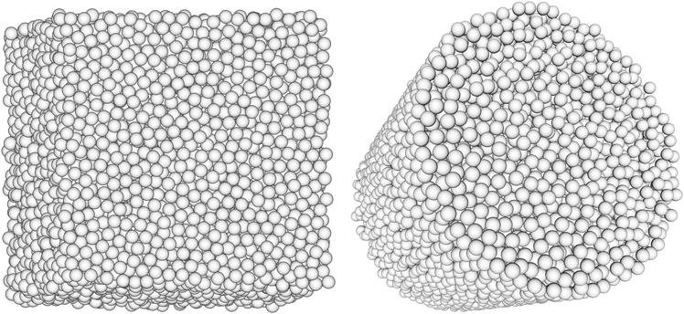
In this section, we describe the computational protocols and experimental methods used to create mechanically stable packings of spheres. Additionally, we introduce a method for the numerical generation of mechanically unstable packings, which are used for comparison. A summary of different preparation protocols can be found in Table 1, two examples of packings are depicted in Fig. 1.

Table 1 Properties of numerical (first three rows) and experimental (last row) packing preparation protocols used in the paper

Protocol	Mechanical stability	Friction	Gravity	Periodic b.c.	No. of particles	No. of packings	Density range
a In the bulk region.
Lubachevsky–Stillinger	Approximately stable	−	−	+	10^4	71	0.560–0.650
Makse	Stable	+	−	+	10^4	13	0.551–0.637
Diluted	Unstable	−	−	+	10^4	36	0.550–0.650
Fluidized bed	Stable	+	+	−	1903–2053^a	503	0.570–0.592

---

Fig. 1 Example of a computer-generated and a reconstructed packing. Left: Computer-generated Lubachevsky–Stillinger packing at the density φ = 0.65. Right: Reconstructed fluidized bed packing (flow rate Q = 167 μl s⁻¹) with the density φ = 0.5784 in the bulk region.

2.1 Lubachevsky–Stillinger packings

The Lubachevsky–Stillinger (LS) algorithm^85,86 simulates Newtonian dynamics and elastic collisions of hard spheres under a vacuum with zero gravity, while at the same time the spheres grow (or, equivalently, the box is contracted). The algorithm terminates when the non-equilibrium reduced pressure (compressibility factor)^68,87 reaches a certain threshold (10¹²). After termination, the final configuration of the particles, i.e. their coordinates and radii are stored as one packing. The volume fraction of this packing can be controlled by the compression rate of the box; for low enough compression rates the packings become crystalline.

The packings generated by the LS algorithm contain 10⁴ monodisperse frictionless spheres, residing in a cubic box under periodic boundary conditions. Using the code by Skoge et al.⁶⁸ we created packings in a density range φ = [0.565–0.65],§ corresponding to compression rates between 0.2 and 4.6 × 10⁻⁴.

The mechanical stability of the resulting packings is not automatically enforced by the Lubachevsky–Stillinger algorithm. An infinite equilibrium pressure would be equivalent to mechanical stability even for frictionless particles,⁸⁸ but (i) the pressure that is tracked during the algorithm operation is inherently non-equilibrium and (ii) the dynamics is stopped at a finite pressure threshold where the particles are still moving.

However, as our analysis later will show that the properties of these packing are close to the properties of fully arrested packings. This can also be seen by expanding all particles with a single linear strain step of 10⁻⁴ and counting particle intersections as contacts.¹⁹ The average contact number Z determined in such a way is larger than the isostatic, frictional limit of 4 in all our simulations. This is not a generic feature of numerically produced packings and other protocols produce packings with φ < 0.65 only with Z ≈ 0.⁶⁵

2.2 Makse packings

The next set of packings corresponds to the mechanically stable packings used in the paper by Briscoe et al.,¹⁸ which can be downloaded from ref. 89. This protocol takes Lubachevsky–Stillinger packings and stabilizes them using a discrete element method (cf. Section VI from Supplementary material in ref. 19). During the operation of the discrete element method, the particles are enhanced with Hertzian normal forces and tangential friction. Like Lubachevsky–Stillinger packings, these packings are three-dimensional and reside in cubic boxes with periodic boundary conditions in all directions.

The lowest value of φ = 0.5513 for Makse packings was reached by Briscoe et al. for spheres with a friction coefficient of μ = 10⁴. To avoid mixing of packings created with different parameters, we use in this paper only the subset of their packings created with this value of μ.

2.3 Fluidized bed packings

This experimental dataset addresses the question of mechanical stability by preparing loose packings of glass spheres which are (a) completely at rest and (b) stable under a finite pressure, i.e. their own weight.

The sample consists of 14 000 monodisperse quartz glass spheres with a diameter of 351 ± 0.5 μm from Sandoz Fils S.A. Individual packings are created by fluidizing the particles with flow pulses of water in a fluidized bed.¹⁰ Then X-ray tomographies of the samples were obtained at the European synchrotron radiation facility (ESRF) in Grenoble at beamline ID15A. The high X-ray flux allowed us to take a full tomogram with up to 1500 projections in less than 20 seconds in the monochromatic X-ray beam. This enabled us to gather several hundred tomograms (cf.Table 2), each representing a separate packing configuration.

Table 2 Experimental parameters for the fluidized bed packings. The column “number of particles” refers to the analysed bulk region

Flow rate, Q (μl s^−1)	Flow duration (s)	Resolution (μm per voxel)	No. of particles	No. of packings	Average bulk density, φ	Density range
a For this set of packings, we were slightly varying the radius of the bulk region to ensure an equal amount of spheres in the latter.
250	10	12	1909–1962	263	0.574	0.570–0.579
167	10	12	1903–1968	173	0.575	0.571–0.580
150	15	18	2053^a	67	0.588	0.581–0.592

---

The fluidized bed consists of a cylindrical tube with an inner diameter of 8 mm or 22.7 particle diameters. The inner surface of the tube was roughened manually to prevent crystallization near the boundary. During preparation, the bed is expanded by a short water pulse (10 or 15 s), then it sediments for 10 seconds. After sedimentation, while the bed is in a stationary state, a tomogram is taken. Then the cycle “water pulse–sedimentation–reconstruction” is repeated.

The fluidization parameters used in three different experiments are listed in Table 2. We will subsequently refer to the three experiments according to their flow rate Q, i.e. Q_250, Q_167, and Q_150. Table 2 lists also the average φ of all packings, as well as the φ interval in each set.¶ In agreement with previous work¹⁰ we find that lower flow rates create denser packings. By comparing successive tomograms, we validated that even the lowest Q used in the experiments was sufficient to create a new packing configuration with each pulse. To ensure that beds are not disturbed by rotation during tomography scans, we took two tomograms without issuing a water pulse in-between. The resulting difference in particle positions is smaller than our overall accuracy of approximately 0.1 voxel.

The sphere positions were first detected as the centers of mass of the binarized images; this estimate was then improved by finding the cross correlation maximum with a set of grey-scale template shifted in 0.1 voxel steps along all axes.|| Together with the good monodispersity of the quartz spheres this method results in the, to our knowledge, the best published accuracy of experimental particle positions. This claim is made quantitatively in Appendix 6.1, where we demonstrate the first peak of the pair correlation function.

We restrict our subsequent analysis to the bulk regions of fluidized bed packings, i.e. we analyse only particles whose centers are at least 2 mm (respectively, 5.6 particle diameters) away from the cylinder boundary. In addition, we exclude a layer of two particle diameters at the top and bottom of every reconstructed packing.

We find that we still have to exclude 34% of the packings from our analysis because their pore-size distributions show features which both differ from theoretical predictions and are not seen in any of the computer-generated packings. We attribute these unexpected features to image processing artefacts which distort the positions of a small number of spheres. Details on how experiments with untypical pore-size distribution are identified can be found in Appendix 6.2.

2.4 Diluted packings

These types of packings are intended to illustrate the effect of missing mechanical stability. They are created by first taking a reference Lubachevsky–Stillinger packing at a density φ = 0.65. Then, particle positions and box size are proportionally scaled to obtain densities in a desired range φ = 0.55–0.65. The resulting packings have contact numbers Z equal to zero and are therefore not mechanically stable.

3 Computing an upper bound on the Edwards entropy

3.1 Theoretical approach

In this subsection, we discuss our modified version of the Widom particle insertion method^82–84 which allows us to compute an upper bound on the Edwards entropy per particle. The main idea here is that we enforce the condition of mechanical stability by (a) starting from packings which already possess these properties and (b) by inserting particles in such a way that they will have enough contacts to be mechanically stable themselves.

3.1.1 Edwards entropy. Ignoring the contact forces, each packing configuration of N monodisperse spheres can be represented as a point in a 3N-dimensional packing phase space (3 coordinates per particle center). If the side lengths of the packing box are L_x, L_y, and L_z, the total phase space volume is equal to V_tot = (L_xL_yL_z)^N.

Packing preparation protocols can be described in two equivalent ways: either the volume of the box is decreased, or the particle diameter is increased. The former is more equivalent to experimental methods where fixed-size particles “settle” from an expanded state into a final volume. The latter is normally used in numerical protocols.

We will assume in the following discussion monodisperse packings** that are prepared by increasing the particle diameters: starting from an arbitrary low density configuration in the phase space, the protocol changes the particle positions (moving the configurational point in the phase space) and at the same time increases the particle diameter until they reach a configuration that is mechanically stable for a given friction coefficient.

Then configurations with the same final particle diameter can be grouped into equivalence classes if these configurations can be obtained from one another by (i) continuous symmetry operations (translational or—in the case of cylindrical or spherical boundaries—rotational symmetries);⁸⁸ (ii) rattler displacements.

Thus, the entire phase space can be divided into (protocol-dependent) countable⁸¹ basins of attraction of equivalence classes of mechanically stable configurations with different particle volume fractions (densities). For frictionless particles, basins of attraction can be produced, among other protocols, by “Stillinger quenches” (quenches that try to increase particle diameters as fast as possible).^90,91

In order to investigate the “number of mechanically stable states” at a given particle diameter D or equivalently volume fraction φ, we need to operate with the density of states. It will be more convenient to investigate the number of states in a small interval of final particle diameters D.

If N is the number of particles, V is the box volume, Ω_i is the volume of the phase space of a basin of attraction, and D_i is its final particle diameter, we can write the total volume of the basins of attraction with D_i ∈ [D;D + dD) as

and the probability to encounter a state i in the interval of final diameters [D;D + dD) asThus, we can write the entropy of mechanically stable states with D_i ∈ [D;D + dD):where accounts for indistinguishability of particles.^36,81

If we assume equiprobability of stable states,^36,41i.e. the equality of all Ω_i, the Edwards entropy becomes S = ln(C/N!) where C(N,V,D,dD) is the number of mechanically stable configurations with D_i ∈ [D;D + dD).

Switching back to a more experimental view we assume now that the final particle diameter is equal to the initial one but the box is rescaled to match the final density. This leads to a range of accepted box linear dimensions [L,L + h) instead of a range for accepted particle diameters, where h can be termed a “granular Planck length”.

It will be convenient for the discussion below to allow particle centers to move inside the Planck volumes of size h³. That is the entire phase space will be split into hypercubes of volume h^3N and a hypercube is considered mechanically stable if it contains at least one mechanically stable configuration. The number of mechanically stable hypercubes will be equal to C(N,V,D,h) for a sufficiently small h (if h is too big, one hypercube may contain several mechanically stable configurations). Again, hypercubes shall be merged into equivalence classes. From now on D and h are considered fixed and we omit them from the list of parameters.

We can also define a probability to sample a correct (mechanically stable) configuration among all possible configurations as

p_correct(N,V) = C(N,V)h^3N/V^N. (5)

Then the Edwards entropy can be expressed as .

3.1.2 Widom's insertion method. To estimate C(N,V), we adapt the Widom particle insertion method^82–84 to granular systems. Let us keep the volume of a packing V fixed, but add one more particle to the packing of N particles which is in the configuration X_i, where i = 1…C(N,V). We can then define K_i as the number of possible positions in a packing to insert the N + 1th particle in this packing so that (a) there is no overlap with already present particles and (b) the additional particle is itself in a mechanically stable position. This second condition is equal to the requirement that the N + 1th particle has in average at least the isostatic number of contacts with its neighbors.

The number of all correct configurations C(N + 1,V) can thus be estimated as

C(N + 1,V) ≥ K₁ + K₂ + ⋯ + K_C(N,V) = C(N,V)〈K〉, (6)

where the average is over all correct configurations for the (N,V) system. The inequality stems from the fact that some unstable configurations of N particles can become stable if we add the N + 1th particle, and we miss them. In Section 4.4 we give an estimate for the prevalence of such configurations.

We can now introduce the average insertion probability (into an already stable packing):

Eqn (6) is then transformed into

By combining eqn (4) and (8) we obtain

By combining eqn (5) and (8), we could also derive an equivalent expression for p_correct(N,V):

p_correct(N + 1,V) ≥ p_correct(N,V)〈p_insert〉. (10)

We immediately derive from eqn (9)

We will later use N₂, the larger N, as a reference point, so we express S(N₁,V) through S(N₂,V) and also make substitutions N₁ → N and N₂ → N₀:

An important step in the Widom method is to assume that the 〈p_insert〉 can be represented by p_insert from a single system:

〈p_insert〉 = p_insert. (13)

A sufficient condition for eqn (13) in classical systems is that an examined single packing is in equilibrium. But the discussion above does not necessarily require packings to be equilibrated and does not imply ergodicity. The only requirement is that packings produced by a given protocol at given (N,V) possess similar properties and are in this sense “typical”, so that we can apply eqn (13).††

It will be more natural to switch in eqn (12) to the entropy per particle, s = S/N. This quantity shall depend only on the particle volume fraction φ and h. We also replace N with φ in the integration in eqn (12) through φ = NV_sp/V, where V_sp is the sphere volume. We thus arrive at the master equation (where we use the subscript “ub” to denote the upper bound)

A natural choice for φ₀ in eqn (14) is the point where s₀ is zero: the entire term will then vanish. As discussed in the introduction, the highest possible value of φ for packings with suppressed crystallization is the Glass Close Packing limit φ_GCP. At this endpoint of the amorphous branch of the hard sphere phase diagram⁵⁵ there will be only one densest configuration (up to particle permutations, symmetry operations, and possibly up to rattler displacement). All configurations equivalent up to continuous symmetry operations, such as translations, and rattler displacements are already combined by design into equivalence classes. The number of discrete symmetry operations is the same for any N, it is 48 for a fully periodic cubic box (symmetry order of the octahedral symmetry O_h).⁹⁴ The density φ_GCP can be expressed through the box size L_GCP with . If we select h so that the last interval of box volumes (L_GCP − h,L_GCP] in eqn (4) contains only the GCP configuration, then we can compute s₀ as s₀ = ln(48N!/N!)/N = 48/N, which in the thermodynamic limit will go to zero. We note that this selection of the reference point leaves h hidden in s_ub (cf.eqn (4)), and the value of h is essentially unknown.

3.1.3 Remarks on Widom's method. Eqn (8) represents the essence of the Widom particle insertion method^82–84 for granular matter and is equivalent to eqn (1) in ref. 82 or eqn (5) in ref. 84. These equations are derived for classical thermodynamic systems with arbitrary potential. Eqn (2.2) in ref. 95 is the expression of the same idea, but specifically for the hard-sphere fluid.

A more detailed mathematical discussion of the Widom method can be found in our accompanying paper.⁹⁶ We validate there our procedure⁶⁵ for estimating p_insert for the hard-sphere fluid. The same procedure, extended for granular systems, is presented in the next section.

For classical systems, all the equations in the previous section are exact. For such systems one also measures the volume of valid configurations, not their number. The phase space for classical systems contains additional kinetic degrees of freedom, but switching to excess quantities eliminates them from equations. Thus, it is more common to express eqn (10) through the excess chemical potential Δμ, Δμ/kT = −ln(〈p_insert〉).^82,84,92,95Eqn (14) looks even simpler in excess quantities, . We validate this form of equation in the accompanying paper.⁹⁶Eqn (10) requires minimal changes to switch to classical systems, we only have to replace inequality with equality:

p_correct(N + 1,V) = p_correct(N,V)〈p_insert〉. (15)

We illustrate eqn (15) in Fig. 2 for the case of a one-dimensional hard-sphere fluid with N = 2 (i.e. ignoring the requirement of mechanical stability). In this case the N + 1 phase space is only three-dimensional and can therefore be still visualized.

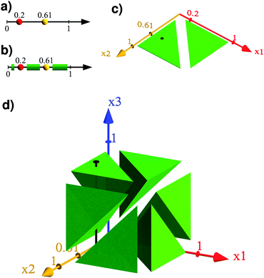Fig. 2 Visualization of the Widom method (eqn (15)) using a one-dimensional hard-sphere system, and ignoring the condition of mechanical stability. Panel (a) shows a specific two-particle system in a one-dimensional box extending from 0 to 1. Panel (c) displays the available phase space p_correct(2,V), for arbitrary positions of the two particles, as a green area. The specific system of panel (a) is here indicated as a black dot. Panel (b) visualizes in green the available space for the insertion of a third particle in this specific system without overlap with the first two particles. The green area in panel (d) shows the available phase space of the generic three-particle system. Panel (b) coresponds to an one-dimensional hyperslice of this phase space, it is indicated by the black vertical line. The Widom insertion method now corresponds to the statement that one can compute p_correct(3,V) (the fraction of the green volume in 3D in panel (d)) by multiplying p_correct(2,V) (the fractiton of the green area in panel (c)) with p_insert (the fraction of the green length in panel (b)).

Both s and s₀ in eqn (14) contain h (cf.eqn (4)). Thus, the presence of additional h³ there, as well as of V_sp, can be daunting. We note though that V_sp and h³ in eqn (14) are also both hidden in p_insert and are cancelled out. The presence of h³ follows directly from eqn (7). To understand the dependence of p_insert on V_sp, we notice that K from eqn (7) shall be extensive, i.e. K = Nα(φ), and thus , where D is the particle diameter. We will discuss the implications

p_insert ∼ h³(if h → 0), p_insert ∼ D⁻³ (16)

during the estimation of p_insert below. We believe that it is easier to use p_insert instead of α, but V_sp and h³ in eqn (14) shall be exactly the ones used for the estimation of p_insert.

In classical systems the Widom insertion method is normally used in conjunction with the canonical ensemble.^82–84 This is in principle also possible for the granular case: the ratio C(N,V)/h from eqn (4) represents the density of states, which can also be written as ,^2,41 where the summation of delta-functions is over all mechanically stable states. Switching to the canonical ensemble would remove the delta-functions and the unknown hidden h from eqn (14). In the canonical ensemble the partition function Z_N looks like , where χ is the compactivity. Here the compactivity controls the average volume that the small subsystem gains when it is generated (along with a large “bath” of particles) with a certain packing preparation protocol. However, as the correct method to measure compactivities is still an active area of research,³⁴ we abstain here from switching to the canonical ensemble.

We also mention that for particles with soft shells, when mechanically stable states are defined by local elastic energy minima and shells are wide enough to avoid zero energy plateaus at any relevant φ, entropy can be defined as the number of states at every φ even in the microcanonical ensemble.^36,81 It would also remove the delta-functions and unknown hidden h from eqn (14). We do not consider such particles in this paper.

3.1.4 How to estimate the insertion probability p_insert. The insertion probability is measured by randomly placing a large number of points inside the packing and then determining for each point the distances to the surfaces of several nearest particles (cf.Fig. 3). This way we measure for each random point a set of r_z, which denote the distance from the point to the zth closest particle surface (the range of z is discussed below).

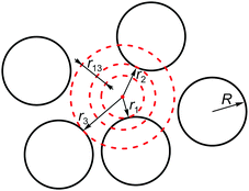Fig. 3 Schematic illustration of distances from a random point to the closest particle surfaces in two dimensions.

The idea is now to estimate the correct insertion probability of a “virtual” particle with a given number of contacts by giving conditions on these distances. We assume two particles to be in contact if the closest distance between their surfaces does not exceed some small arbitrary constant δ. To insert a virtual particle with an arbitrary radius r₀ having ≥z contacts, we require two conditions: (a) the particle has to fit in, i.e. r₁ = r₀, (b) it has to touch at least z particles, i.e. r_z ≤ r₁ + δ.

The last condition will be easier to discuss if we operate with relative distances r_1z = r_z − r₁ for z > 1 (cf.Fig. 3). By inserting a large number of virtual particles we then measure the probability density functions for the distributions of r₁ and r_1z, which we denote as f(r₁) and g_1z(r₁,r_1z), respectively (note that g_1z depends on r₁ as well). f(r₁) is described in many papers as pore-size distribution.^97–105 We also operate with the conditional probability density g_1z(r_1z|r₁) to find a given value r_1z when the distance to the first closest sphere is r₁: g_1z(r_1z|r₁) = g_1z(r₁,r_1z)/f(r₁). We denote the corresponding cumulative distributions as G_1z(r₁,r_1z) and G_1z(r_1z|r₁).

The probability density h_z(r₀) to insert a particle with radius r₀ and at least z contacts can be computed using the two conditions named above as

h_z(r₀)dr₀ = Pr{r₁ ∈ [r₀,r₀ + dr₀), r_1z ∈ [0,δ)} = f(r₀)dr₀ × Pr{r_1z ∈ [0,δ)|r₁ = r₀}. (17)

Here, by definition,

Pr{r_1z ∈ [0,δ)|r₁ = r₀} = G_1z(δ|r₀). (18)

G_1z(δ|r₀) can be interpreted as “zero distance probability”, i.e. the probability to have at least z contacts for a pore with radius r₀. By combining eqn (17) and (18), we obtain

h_z(r₀) = f(r₀)·G_1z(δ|r₀). (19)

If R is the radius of “real” particles, then h_z(R)dR is the probability for an inserted particle to have at least z contacts and the radius in the range [R,R + dR).

To enforce mechanical stability for inserted virtual particles, we have to choose a relevant z. The two immediate choices are z = 3 and z = 4. It is known that 4 is the minimal possible average coordination number in mechanically stable packings (realized in packings with infinite friction). The contact number distribution is never a “delta-function”,¹⁹ so non-rattler particles with three contacts are inevitable, though not every configuration of three contacts will be mechanically stable. We will denote the correct minimal z as z_min, but will discuss the choice between z_min = 3^30,106,107 and z_min = 4^108,109 in the Results Section 4.

At this point, we can estimate the probability p_insert from eqn (14) to correctly insert a particle in a packing:

p_insert = dR·f(R)·G_1zmin(δ|R). (20)

The distributions f(R) and G_1z(δ|R) depend all implicitly on the volume fraction φ and thus determine the dependence of p_insert on φ.

3.1.5 Scaling of p_insert with h and D. Because we define mechanically stable configurations up to Planck volumes h^3N, particle centers are allowed to move inside their Planck volumes h³ without invalidating the condition of mechanical stability of configurations. It implies that both dR and δ shall be equal to the Planck length assumed in eqn (14). In the following we will use h = 2 × 10⁻⁷:

dR = δ = h = 2 × 10⁻⁷. (21)

Eqn (16) implies that p_insert scales as h³ and D⁻³. Because h is present as dR in eqn (20) explicitly, G_1zmin(h|R) shall conform to

G_1zmin(h|R) ∼ h² (if h → 0). (22)

We will use this restriction in Section 4.1. To examine scaling of eqn (20) with D, we shall express f(R) and G_1zmin(δ|R) through dimensionless distributions and , respectively. From the elementary probability theory it follows that and thus . Through rewriting g_1z(r₁,r_1z) in the same way (applied to both arguments) and dividing by f(R), we can write . Thus, . Note that we had to change the limits of integration. It means that whenever we require that G_1z(h|r₁) ∼ h² (i.e. G_1z(h|r₁) = A(D)h²), it implies that . Thus, , and scaling with both h and D is correct, if eqn (22) indeed holds as expected. We will imply D = 1 a.u. from now on.

3.2 Overview of data analysis steps

In finite size packings, such as our experiments and simulations, neither f(R) nor G_1z min(h|R) can be measured directly. The maximum observed value for r₁ (radius of inserted particle) is ∼0.4R. Moreover, the minimum values of r_1zmin (and generally of all r_1z) are much larger than h even for r₁ < 0.4R. To fix this issue, we fit the obtained values of f(r₁) and extrapolate r₁ → R. Additionally, we need to fit G_1z(r_1z|r₁) for z = z_min and extrapolate r_1z → h and r₁ → R. To make our results more general, we will present a method applicable for all z from 3 at least to 11.

The entire procedure to estimate the upper bound of the Edwards entropy according to eqn (14) contains therefore the following steps:

(1) We uniformly generate 10⁷ random points in all packings. For each point, we measure distances to the closest particles, with indices z from 3 to 11 (though in principle we will need only z = z_min).

(2) We fit f(r₁) and extrapolate it to r₁ = R (cf. the next section for the fitting procedures).

(3) We distribute values of r₁ into bins. Initially we use 100 bins of equal size, then merge some of them to ensure that the minimum number of points in each bin is 80. For each bin (i.e. for each r₁), we fit g_1z(r_1z|r₁) as a function of r_1z. Then we extrapolate it to r_1z = 0, and estimate G_1z(h|r₁).

(4) For each value of z, we fit G_1z(h|r₁) as a function of r₁ and extrapolate it to r₁ = R.

(5) Finally, we insert f(R) and G_1zmin(h|R) into eqn (20) to obtain p_insert at each φ and insert p_insert into eqn (14) to obtain the upper bound of the Edwards entropy per particle s_ub.

3.3 Details of the fitting and extrapolation steps

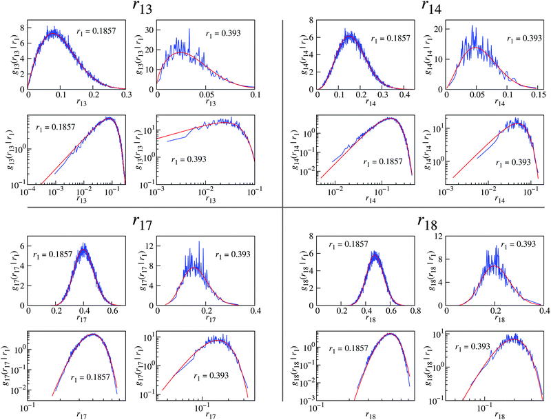
In this subsection we will justify our choice of fit functions used for the extrapolation steps. In order to demonstrate better statistics we present in the figures in this section the combined distributions g_1z(r_1z|r₁) from 39 fluidized bed packings with φ = 0.587 ± 0.003.

3.3.1 Fitting f(r₁) and extrapolating it to r₁ = R. As in our previous work⁶⁵ we followed Schenker et al.¹⁰³ and fitted f(r₁) with the truncated Gaussian distribution:¹¹⁰

Theoretical results^97–99 predict that f(r₁) is of the form A exp(ar₁³ + br₁² + cr₁ + d), of which eqn (23) is a special case. The validity of the function from eqn (23) was already demonstrated in our previous paper⁶⁵ (see Fig. 2 in that reference).

The normalization constant C in eqn (23) corresponds to the fact that the probability for a pore to appear in the interparticle void space is 1 − φ. It can be computed using . Fits were performed using the maximum likelihood method for a truncated Gaussian distribution.¹¹⁰

3.3.2 Fitting g_1z(r_1z|r₁) and extrapolating it to r_1z = 0. We found that the two-parameter probability distribution known as the Nakagami distribution¹¹¹ provides the best fits for all the distributions g_1z(r_1z|r₁) computed in experiments and simulations (z = 3…11). The Nakagami probability density function f_x(x;m,Ω) is defined as It is a two-parameter distribution, which is defined for x ∈ [0,+∞). At x = 0, it grows as x^2m−1. At large x, it decays as exp(−x²). Examples of the distribution g_1z(r_1z|r₁) as a function of r_1z for contact numbers z = 3, 4, 7, and 8 and their fits with the Nakagami distribution are presented in Fig. 4.

Fig. 4 The experimentally obtained g_1z(r_1z|r₁) (blue lines) are fit well with Nakagami distributions (red lines). The data represent 39 combined fluidized bed packings (Q_150) with an average φ of 0.585. Distributions for r₁₃, r₁₄, r₁₇, and r₁₈ (respectively z = 3, 4, 7, and 8) are displayed. Each fit is shown twice, in a linear (top) and in a log–log scale (bottom). The particle diameter is normalized to unity.

As there is no first-principle based theory supporting our choice of the Nakagami distribution, we have tried to fit other distributions with support x ∈ [0,+∞) and f_x → 0 at x → 0. The result is that one-parameter distributions do not have enough degrees of freedom to fit all the different g_1z(r_1z|r₁) curves, while three-parameter distributions are too flexible and fits are not robust. Among the examined two-parameter distributions, the gamma and Rice distributions possess shapes similar to the observed g_1z(r_1z|r₁), but the quality of fit is inferior to the Nakagami distribution. For example, the gamma distribution decays at large x with exp(−x) which is too slow.

From the parameters m and Ω from the Nakagami fit we compute the zero distance probability G_1z(h|r₁), which is the cumulative density function of the Nakagami distribution F_x at x = h. The latter has the following analytical expression

Here, P(s,x) is the regularized incomplete gamma function, is the lower incomplete gamma function, and Γ(m) is the gamma function. Thus, we can express G_1z(h|r₁) as

3.3.3 Fitting G_1z(h|r₁) and extrapolating it to r₁ = R. The last step is to extrapolate the zero distance probability G_1z(h|r₁) to r₁ = R. Fig. 5 shows G_1z(h|r₁) for contact numbers 3 and 8 as blue lines. In the absence of a theoretically-derived fit function we use a heuristically motivated least-squares fit of the form:

ln[G_1z(h|r₁)] = d − exp[ar₁² + br₁ + c] (27)

for all points with r₁ ≥ 0.1, which is the lowest boundary for which the fit is still applicable for all coordination numbers z. Corresponding fits are depicted as the red lines in Fig. 5.

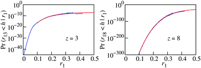Fig. 5 Extrapolating the zero distance probability G_1z(h|r₁) (blue lines) using eqn (27) (red lines). G_1z(h|r₁) ≡ Pr(r_1z < h|r₁) is the probability that a pore with radius r₁ will have exactly z contacts with real particles in a shell of width h. The data represent 39 combined fluidized bed packings (Q_150) with an average φ of 0.585. The particle diameter is normalized to unity, the extrapolation is therefore to r₁ = 0.5.

We confirm that the estimates of p_insert do not change qualitatively if G_1zmin(h|R) is determined by averaging the three G_1zmin(h|r₁) values with the highest available r₁.

4 Results and discussion

4.1 Scaling of zero-distance probabilities G_1z(h|R) with h

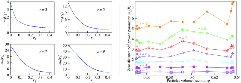
Eqn (22) requires that G_1zmin(h|R) ∼ h² for sufficiently small h. It follows from the form of the Nakagami distribution (eqn (24)) that for small x the cumulative Nakagami distribution F_x(x;m,Ω) scales as x^2m. For a given protocol, m is a function of z, φ, and r₁. Thus, eqn (22) implies that m_zmin(r₁ = R) = 1 at all φ (the Nakagami distribution is then transformed into the Rayleigh distribution).

To test the behaviour of m_z, we build m_z(r₁) from the Nakagami fits for the combined g_1z(r_1z|r₁) distributions for the 39 Q_150 packings used in Section 3.3 (with φ = 0.587 ± 0.003). The results are presented in the left panel of Fig. 6.

Fig. 6 Left: Nakagami growth parameter m vs. the pore radius r₁ for different contact numbers z. The data represent 39 combined fluidized bed packings (Q_150) with an average φ of 0.585. We extrapolate m_z(r₁) to the particle radius r₁ = R = 0.5 by averaging the three right-most points of each plot. Right: Asymptotic Nakagami growth parameters m_z(r₁ = R) vs. the particles volume fraction φ for different contact numbers z. Presented are the data from the Makse packings.

As before, to estimate m_z(R) we have to extrapolate r₁ to R. For z ≤ 6, the m_z(r₁) plots visually reach asymptotes for the largest values of r₁ for all the packings that we used. Thus, to estimate m_z(R) we simply take an average of the last three values of m_z(r₁). The plots m_z(R) vs. φ for the Makse packings are presented in the right panel of Fig. 6.

The values with z ≤ 8 show no systematic dependence on φ in Fig. 6. Thus, we can compute their averages. The estimates 〈m_z(R)〉_φ for the Makse packings are (z = 3…11): 0.792, 1.238, 1.761, 2.424, 3.185, 4.128, 5.883, 8.412, and 11.923. The values with z > 6 are very crude estimates.

Both m₃(R) and m₄(R) are around unity, which is in line with the requirement m_zmin = 1. None of them is equal to unity though. One possible explanation is that our estimates for m₄(R) are still too high and the plot m₄(r₁) continues to decrease with r₁ (like plots m_z(r₁) do, cf.Fig. 6), so that it eventually reaches the value m₄(r₁) = 1 at r₁ = R. This effect will be incorporated into the extrapolation of G_1z(h|r₁) with r₁ → R (cf.Fig. 5), if this extrapolation is correct. At the same time, m₃(R) does not seem to reach the value 1. Thus, we will prefer z_min = 4 to z_min = 3.

The proximity of m₃(R) and m₄(R) to unity and their independence from φ, as expected from general scaling considerations, demonstrate the validity of our approach and the correctness of fits, though we never incorporated these requirements during the fitting procedure.

4.2 Zero-distance probabilities G_1z(h|R)

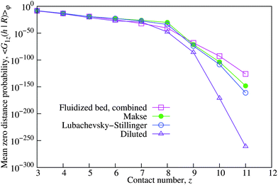
Fig. 7 shows that the zero distance probabilities G_1z(h|R) have no systematic dependence on φ for z ≥ 3. The data shown here represent the Makse packings, but the Lubachevsky–Stillinger packings are qualitatively similar. This result corresponds to the statement that the local structure of large pores in a packing remains unchanged over the entire density range of random monodisperse packings.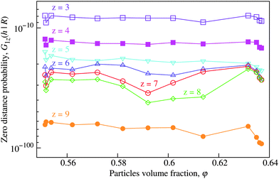

Fig. 7 The zero-distance probabilities G_1z(h|R) for the different contact numbers z show no systematic dependence on the volume fraction φ. Presented are the data from the Makse packings.

Because the values of G_1z(h|R) do not change systematically with φ, we can compute an average 〈G_1z(h|R)〉_φ by averaging over the whole volume fraction range. The corresponding results for all the protocols are shown in Fig. 8. For the fluidized bed packings, we combined the data for all the values of flow rate Q prior to averaging.

Fig. 8 Zero-distance probabilities 〈G_1z(h|R)〉_φ averaged over the whole range of volume fractions.

Differences between the protocols become only apparent for z > 5. Among the numerical protocols, the Makse packings have the highest zero distance probabilities, followed by the Lubachevsky–Stillinger packings. Zero distance probabilities for the diluted packings are significantly low, especially for z > 7. This sequence corresponds to the “degree of mechanical stability” of the packings: the Makse packings are mechanically stable, the Lubachevsky–Stillinger packings are close to being stable, while the diluted packings have large interparticle gaps by design. Fluidized bed packings demonstrate even higher “degree of mechanical stability” than the Makse packings for z > 9, but there is a crossover in the order of lines between z = 8 and z = 9. Fig. 8 demonstrates that G_1z(h|R) might therefore be an interesting tool to quantify the proximity to mechanical stability.

4.3 Insertion probabilities p_insert

Fig. 9 shows the results for p_insert computed with z_min = 4. We have excluded here the diluted packings, because their average coordination number is zero.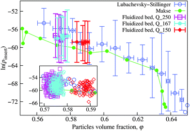

Fig. 9 All the estimates of p_insert(φ) decrease monotonously with the volume fraction φ. Results are computed using eqn (20) with z_min = 4. LS and fluidized bed data points were binned in the main plot. Vertical error bars represent 95% prediction intervals in bins, horizontal error bars represent minimum and maximum densities in bins. Data were grouped to ensure 5, 66, 43, and 17 packings in the bins for the LS, Q_250, Q_167, and Q_150 lines, respectively. The inset shows all the individual experiments.

Two main results are shown in Fig. 9. First, within error bars the Makse, LS, and fluidized bed packing agree quantitatively in their p_insert, without any fit parameter. Interestingly, the agreement between the only approximately stable LS and fully stable fluidized bed packings is better than with the also fully mechanically stable Makse packings. We will come back to this point in Section 4.4. Second, p_insert exhibits a maximum at RLP and then decays monotonously with increasing φ.

4.4 Upper bound on the Edwards entropy per particle

With p_insert(φ) at hand, we can compute the estimates of the Edwards entropy per particle s_ub according to eqn (14). As discussed in Section 3.1.2, we assume here that s₀ becomes zero at the Glass Close Packing limit φ_GCP = 0.65. Because the Makse packings are only defined up to a maximum φ of 0.637 and because the p_insert(φ) of the Lubachevsky–Stillinger packings agrees better with the experimental data in Fig. 9, we will use the Lubachevsky–Stillinger packings to compute the upper bound on the Edwards entropy displayed in Fig. 10. At least in the range 0.570 < φ < 0.592, s_ub can also be computed from the fluidized bed data, using a corresponding Lubachevsky–Stillinger value of s at φ₀ = 0.592 as a reference value s₀ in eqn (14). These results are also shown in Fig. 10, it is within our accuracy indistguishable from the Lubachevsky–Stillinger derived values.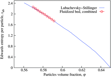

Fig. 10 The upper bounds on the Edwards entropy per particle s_ub(φ) decrease monotonously with the volume fraction φ. Results are computed using eqn (14) with z_min = 4, p_insert is taken from Fig. 9.

The values of s_ub exhibit a maximum at RLP and decay monotonously with increasing φ. This behaviour supports previous numerical^19,112 and experimental³⁴ analyses. It also agrees with the idea that s drops sharply to zero (in the canonical ensemble) for φ below RLP.

More generally, this method to compute s_ub will allow for the first time to test the different protocols that have been suggested to measure the configurational temperature X.^{5,10,15–18,20,25,32–34} Moreover, our approach should be extendable to bidisperse systems, which will allow us to test the idea that segregation in dense bidisperse systems is controlled by configurational entropy.^{7,31,113–116}

The origin of the difference between s(φ) and s_ub(φ) is configurations which gain stability only due to insertion of an additional particle. To account for such configurations, we can formally rewrite eqn (6) as

C(N + 1,V) = C(N,V)〈K〉α(N,V), (28)

where the a priori unknown function α(N,V) measures how many configurations of the (N,V) ensemble will become stable only after adding one more particle. This implies α(N,V) ≥ 1 with α(N,V) = 1 only in the case that there are no “fluid” configurations which will develop a finite yield stress if a single particle is inserted.

If we keep the definition for the average insertion probability into an already stable packing (eqn (7)) the same, eqn (12) will then be replaced by

which corresponds to the statement that Because α ≥ 1 and N < N₀, this difference will always be positive and it will increase with decreasing φ, i.e. it will be maximum at the RLP limit.

A qualitative estimate for α might be obtained by investigating the case of removing a particle from the packing under consideration. The likelihood that any of the neighbors of this particle becomes unstable will decrease with increasing distance to isostaticity, z − z_iso, which corresponds to the statement that packings close to RLP are the most “fragile”. By analogy, configuration close to RLP should therefore also be the most likely to gain mechanical stability by adding another particle. Thus, we conclude that α will be maximum at the RLP limit. This argument should also allow us to measure α numerically and therefore turn the upper bound into a direct estimate of the Edwards entropy. To do so one needs to measure the probability that removing single particles from given mechanically stable packings will make them lose their stability.

Our analysis does not consider the effects of a finite boundary pressure and by design we have no access to the degeneracy that hyperstatic packings have in the phase space spanned by the contact forces. However, all our packings were comprised from hard particles so that particle positions and contact forces decouple. The numerical packings do so by design, and the fluidized bed experiments were done under a constant pressure small enough that the glass spheres can be considered as perfectly hard: the pressure between two glass spheres at the bottom of a 1 m high column will deform them by approximately 10 nm, which is an orders of magnitude smaller than the vertical surface roughness of typical glass spheres.¹¹⁷ And the grain column in our fluidized bed experiment was only 0.03 m high.

However, the value of RLP, measured with glass spheres, does depend on pressure.⁴³ This means that at least close to the isostatic point also s will show some pressure dependence. This effect originates in the reduced degeneracy in the contact force space; the closer to isostaticity a packing is, the fewer configurations will exist to fulfil certain pressure boundary conditions. An analysis of loose packing created at different pressure levels should provide interesting insights.

Finally, we would like to point out that a generalization of our method to other particles shapes, such as ellipsoids or Platonic bodies, seems feasible.

5 Summary

In this paper, we present a method to compute an upper bound on the Edwards entropy per particle of three-dimensional, mechanically stable hard-sphere packings within a microcanonical ensemble. We modify the Widom insertion method to be applicable for granular systems and also extend our method to estimate particle insertion probabilities for hard-sphere systems using their pore-size distribution to account for the requirement of mechanical stability of the packing. Then we supply these insertion probabilities into the master equation from the Widom method.

We apply this procedure to experimentally obtained and computer-generated packings covering the volume fraction range from 0.551 to φ_GCP ≈ 0.65 (the Glass Close Packing density, according to some estimates). The experimental packings are created with flow pulses in a water-fluidized bed, the numerical packings are prepared using the Lubachevsky–Stillinger algorithm. One subset, taken from the publication of Briscoe et al.,¹⁸ adds an additional discrete element simulation step to obtain fully jammed configurations.

Starting from a minimum at the Glass Close Packing density the upper bound on the Edwards entropy grows monotonically with decreasing volume fraction to reach a maximum around the Random Loose Packing density φ_RLP ≈ 0.55. Because there are by definition no mechanically stable packings below Random Loose Packing, the Edwards entropy shall drop there to zero (in the canonical ensemble).

Additionally, we find that the local structure around pores large enough to fit in another particle does not depend on the volume fraction. This volume fraction independence was quantified by computing the probabilities of the inserted particles to have a given number of contacts.

6 Appendix

6.1 Pair correlation functions for fluidized bed packings

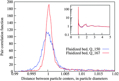
The monodispersity of the particles and the high quality of the particle detection of fluidized bed experiments are demonstrated by the pair correlation functions shown in Fig. 11. The data correspond to individual fluidized bed packings where we have discarded a layer of one diameter thickness along the cylinder walls. While the absolute height of the first peak, which corresponds to particles in contact, depends on the bin size, its width is a testimonial to the quality of the data.

Fig. 11 Pair correlation function for fluidized bed packings. The inset shows the data in a semi-log scale. The bin width is 2 × 10⁻⁴D in the main figure and 2 × 10⁻²D in the inset, except for the points inside the 0.99–1.02D interval, where we use the bins from the main plot. D is the particle diameter.

6.2 Selecting fluidized bed packings

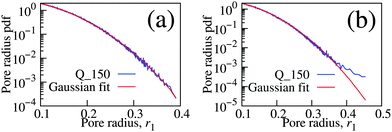
Approximately 34% of the fluidized bed packings were discarded due to the atypical pore-size distributions. Fig. 12 shows two examples. The experiment in panel (b) behaves atypically as the tail deviates from the expected Gaussian curve (eqn (23)) towards higher probability densities. Such a behaviour was neither observed in the computer-generated Makse, Lubachevsky–Stillinger, and diluted packings nor was it observed for the force-biased and Jodrey–Tory packings studied in our previous paper⁶⁵ and by Schenker et al.¹⁰³ Thus, we assume that this atypical behaviour stems from reconstruction artefacts and discards such packings from the calculation of entropies.

Fig. 12 Experimentally obtained pore radii probability density functions (blue lines) and their fits with Gaussian distributions (red lines) for two reconstructed packings: (a) accepted packing; (b) rejected packing. The particle diameter is normalized to unity.

Fig. 12 demonstrates also that the pore-size distribution may serve as an additional indicator of packing reconstruction quality, besides the pair-correlation function discussed in Section 6.1.

Acknowledgements

We thank Sibylle Nägle for creating Fig. 2 and Udo Krafft and Wolf Keiderling for building the fluidized bed setup. X-ray tomographies were performed on the ID15A beamline at the European Synchrotron Radiation Facility (ESRF), Grenoble, France. Computational resources were provided by FZJ (Forschungszentrum Jülich, Germany). The authors would like to acknowledge the funding of the Deutsche Forschungsgemeinschaft (DFG) through the Cluster of Excellence Engineering of Advanced Materials. The French National Research Agency (ANR) is acknowledged for support via EQUIPEX grant ANR-11-EQPX-0031 (project NanoimagesX). We are grateful to the John von Neumann Institute for Computing (NIC) and the Jülich Supercomputing Center (JSC) for the allocation of a special CPU-time grant (NIC project number: 8214, JSC project ID: HMR10).

References

1. N. V. Brilliantov and T. Pöschel, Kinetic Theory of Granular Gases, Oxford University Press, 2004.
2. S. F. Edwards and R. B. S. Oakeshott, Physica A, 1989, 157, 1080–1090.
3. A. Mehta and S. F. Edwards, Physica A, 1989, 157, 1091–1100.
4. R. Monasson and O. Pouliquen, Physica A, 1997, 236, 395–410.
5. E. R. Nowak, J. B. Knight, E. Ben-Naim, H. M. Jaeger and S. R. Nagel, Phys. Rev. E: Stat., Nonlinear, Soft Matter Phys., 1998, 57, 1971–1982.
6. H. A. Makse and J. Kurchan, Nature, 2002, 415, 614–617.
7. M. Nicodemi, A. Fierro and A. Coniglio, Europhys. Lett., 2002, 60, 684–690.
8. R. Blumenfeld and S. F. Edwards, Phys. Rev. Lett., 2003, 90, 114303.
9. H. A. Makse, J. Brujić and S. F. Edwards, in The Physics of Granular Media, ed. H. Hinrichsen and D. E. Wolf, Wiley-VCH, Weinheim, 2004, pp. 45–85.
10. M. Schröter, D. I. Goldman and H. L. Swinney, Phys. Rev. E: Stat., Nonlinear, Soft Matter Phys., 2005, 71, 030301.
11. P. T. Metzger and C. M. Donahue, Phys. Rev. Lett., 2005, 94, 148001.
12. S. F. Edwards, Physica A, 2005, 353, 114–118.
13. M. Pica Ciamarra, A. Coniglio and M. Nicodemi, Phys. Rev. Lett., 2006, 97, 158001.
14. F. Lechenault, F. da Cruz, O. Dauchot and E. Bertin, J. Stat. Mech.: Theory Exp., 2006, 2006, P07009.
15. P. Ribiére, P. Richard, P. Philippe, D. Bideau and R. Delannay, Eur. Phys. J. E: Soft Matter Biol. Phys., 2007, 22, 249–253.
16. S. Henkes, C. S. O'Hern and B. Chakraborty, Phys. Rev. Lett., 2007, 99, 038002.
17. T. Aste and T. Di Matteo, Eur. Phys. J. B, 2008, 64, 511–517.
18. C. Briscoe, C. Song, P. Wang and H. A. Makse, Phys. Rev. Lett., 2008, 101, 188001.
19. C. Song, P. Wang and H. A. Makse, Nature, 2008, 453, 629–632.
20. S. McNamara, P. Richard, S. K. de Richter, G. Le Caer and R. Delannay, Phys. Rev. E: Stat., Nonlinear, Soft Matter Phys., 2009, 80, 031301.
21. G.-J. Gao, J. Blawzdziewicz, C. S. O'Hern and M. Shattuck, Phys. Rev. E: Stat., Nonlinear, Soft Matter Phys., 2009, 80, 061304.
22. S. Henkes and B. Chakraborty, Phys. Rev. E: Stat., Nonlinear, Soft Matter Phys., 2009, 79, 061301.
23. B. P. Tighe, J. H. Snoeijer, T. J. H. Vlugt and M. van Hecke, Soft Matter, 2010, 6, 2908–2917.
24. N. Xu, D. Frenkel and A. J. Liu, Phys. Rev. Lett., 2011, 106, 245502.
25. L. A. Pugnaloni, J. Damas, I. Zuriguel and D. Maza, Pap. Phys., 2011, 3, 030004.
26. R. K. Bowles and S. S. Ashwin, Phys. Rev. E: Stat., Nonlinear, Soft Matter Phys., 2011, 83, 031302.
27. F. Paillusson and D. Frenkel, Phys. Rev. Lett., 2012, 109, 208001.
28. K. Wang, C. Song, P. Wang and H. A. Makse, Phys. Rev. E: Stat., Nonlinear, Soft Matter Phys., 2012, 86, 011305.
29. S.-C. Zhao, S. Sidle, H. L. Swinney and M. Schröter, EPL, 2012, 97, 34004.
30. S. S. Ashwin, J. Blawzdziewicz, C. S. O'Hern and M. D. Shattuck, Phys. Rev. E: Stat., Nonlinear, Soft Matter Phys., 2012, 85, 061307.
31. M. Schröter and K. E. Daniels, 2012, arXiv:1206.4101.
32. R. Blumenfeld, J. F. Jordan and S. F. Edwards, Phys. Rev. Lett., 2012, 109, 238001.
33. J. G. Puckett and K. E. Daniels, Phys. Rev. Lett., 2013, 110, 058001.
34. S.-C. Zhao and M. Schröter, Soft Matter, 2014, 10, 4208–4216.
35. I. G. Tejada, Eur. Phys. J. E: Soft Matter Biol. Phys., 2014, 37, 1–8.
36. D. Asenjo, F. Paillusson and D. Frenkel, Phys. Rev. Lett., 2014, 112, 098002.
37. F. Paillusson, Phys. Rev. E: Stat., Nonlinear, Soft Matter Phys., 2015, 91, 012204.
38. Y. Wu and S. Teitel, Phys. Rev. E: Stat., Nonlinear, Soft Matter Phys., 2015, 91, 022207.
39. V. Becker and K. Kassner, Phys. Rev. E: Stat., Nonlinear, Soft Matter Phys., 2015, 92, 052201.
40. M. Pica Ciamarra, P. Richard, M. Schröter and B. P. Tighe, Soft Matter, 2012, 8, 9731–9737.
41. D. Bi, S. Henkes, K. E. Daniels and B. Chakraborty, Annu. Rev. Condens. Matter Phys., 2015, 6, 63–83.
42. P. Yu, S. Frank-Richter, A. Börngen and M. Sperl, Granular Matter, 2014, 16, 165–173.
43. M. Jerkins, M. Schröter, H. L. Swinney, T. J. Senden, M. Saadatfar and T. Aste, Phys. Rev. Lett., 2008, 101, 018301.
44. M. van Hecke, J. Phys.: Condens. Matter, 2010, 22, 033101.
45. L. E. Silbert, D. Ertas, G. S. Grest, T. C. Halsey and D. Levine, Phys. Rev. E: Stat., Nonlinear, Soft Matter Phys., 2002, 65, 031304.
46. H. P. Zhang and H. A. Makse, Phys. Rev. E: Stat., Nonlinear, Soft Matter Phys., 2005, 72, 011301.
47. K. Shundyak, M. van Hecke and W. van Saarloos, Phys. Rev. E: Stat., Nonlinear, Soft Matter Phys., 2007, 75, 010301.
48. S. Henkes, M. van Hecke and W. van Saarloos, EPL, 2010, 90, 14003.
49. F. M. Schaller, M. Neudecker, M. Saadatfar, G. W. Delaney, G. E. Schröder-Turk and M. Schröter, Phys. Rev. Lett., 2015, 114, 158001.
50. T. Aste, M. Saadatfar and T. J. Senden, J. Stat. Mech.: Theory Exp., 2006, 2006, P07010.
51. A. Baule, R. Mari, L. Bo, L. Portal and H. A. Makse, Nat. Commun., 2013, 4, 2194.
52. A. Baule and H. A. Makse, Soft Matter, 2014, 10, 4423–4429.
53. S. Torquato and F. H. Stillinger, J. Appl. Phys., 2007, 102, 093511.
54. S. Torquato, T. M. Truskett and P. G. Debenedetti, Phys. Rev. Lett., 2000, 84, 2064.
55. R. D. Kamien and A. J. Liu, Phys. Rev. Lett., 2007, 99, 155501.
56. A. V. Anikeenko and N. N. Medvedev, Phys. Rev. Lett., 2007, 98, 235504.
57. M. Bargieł and E. M. Tory, Adv. Powder Technol., 2001, 12, 533–557.
58. K. Lochmann, L. Oger and D. Stoyan, Solid State Sci., 2006, 8, 1397–1413.
59. C. Radin, J. Stat. Phys., 2008, 131, 567–573.
60. Y. Jin and H. A. Makse, Physica A, 2010, 389, 5362–5379.
61. B. A. Klumov, S. A. Khrapak and G. E. Morfill, Phys. Rev. B: Condens. Matter Mater. Phys., 2011, 83, 184105.
62. S. C. Kapfer, W. Mickel, K. Mecke and G. E. Schroder-Turk, Phys. Rev. E: Stat., Nonlinear, Soft Matter Phys., 2012, 85, 030301.
63. N. Francois, M. Saadatfar, R. Cruikshank and A. Sheppard, Phys. Rev. Lett., 2013, 111, 148001.
64. G. Parisi and F. Zamponi, Rev. Mod. Phys., 2010, 82, 789–845.
65. V. Baranau, D. Hlushkou, S. Khirevich and U. Tallarek, Soft Matter, 2013, 9, 3361–3372.
66. V. Baranau and U. Tallarek, Soft Matter, 2014, 10, 3826–3841.
67. V. Baranau and U. Tallarek, Soft Matter, 2014, 10, 7838–7848.
68. M. Skoge, A. Donev, F. H. Stillinger and S. Torquato, Phys. Rev. E: Stat., Nonlinear, Soft Matter Phys., 2006, 74, 041127.
69. W. G. Hoover and F. H. Ree, J. Chem. Phys., 1968, 49, 3609–3617.
70. E. Sanz, C. Valeriani, E. Zaccarelli, W. C. K. Poon, P. N. Pusey and M. E. Cates, Phys. Rev. Lett., 2011, 106, 215701.
71. E. Zaccarelli, C. Valeriani, E. Sanz, W. C. K. Poon, M. E. Cates and P. N. Pusey, Phys. Rev. Lett., 2009, 103, 135704.
72. C. Valeriani, E. Sanz, E. Zaccarelli, W. C. K. Poon, M. E. Cates and P. N. Pusey, J. Phys.: Condens. Matter, 2011, 23, 194117.
73. L. Filion, M. Hermes, R. Ni and M. Dijkstra, J. Chem. Phys., 2010, 133, 4115.
74. P. N. Pusey, E. Zaccarelli, C. Valeriani, E. Sanz, W. C. K. Poon and M. E. Cates, Philos. Trans. R. Soc., A, 2009, 367, 4993–5011.
75. G. Y. Onoda and E. G. Liniger, Phys. Rev. Lett., 1990, 64, 2727–2730.
76. G. R. Farrell, K. M. Martini and N. Menon, Soft Matter, 2010, 6, 2925–2930.
77. J. M. Valverde and A. Castellanos, EPL, 2006, 75, 985.
78. L. E. Silbert, Soft Matter, 2010, 6, 2918–2924.
79. G. W. Delaney, J. E. Hilton and P. W. Cleary, Phys. Rev. E: Stat., Nonlinear, Soft Matter Phys., 2011, 83, 051305.
80. M. Pica Ciamarra and A. Coniglio, Phys. Rev. Lett., 2008, 101, 128001.
81. S. Martiniani, K. J. Schrenk, J. D. Stevenson, D. J. Wales and D. Frenkel, Phys. Rev. E: Stat., Nonlinear, Soft Matter Phys., 2016, 93, 012906.
82. B. Widom, J. Chem. Phys., 1963, 39, 2808–2812.
83. D. Frenkel and B. Smit, Understanding Molecular Simulation: From Algorithms to Applications, Academic Press, San Diego, 2nd edn, 2002.
84. D. J. Adams, Mol. Phys., 1974, 28, 1241–1252.
85. B. D. Lubachevsky and F. H. Stillinger, J. Stat. Phys., 1990, 60, 561–583.
86. B. D. Lubachevsky, J. Comput. Phys., 1991, 94, 255–283.
87. G. A. Mansoori, N. F. Carnahan, K. E. Starling and T. W. Leland, J. Chem. Phys., 1971, 54, 1523–1525.
88. Z. W. Salsburg and W. W. Wood, J. Chem. Phys., 1962, 37, 798–804.
89. H. Makse, Software and Data|Hernan Makse, http://www-levich.engr.ccny.cuny.edu/webpage/hmakse/software-and-data/.
90. F. H. Stillinger and T. A. Weber, Phys. Rev. A: At., Mol., Opt. Phys., 1982, 25, 978–989.
91. F. H. Stillinger, Science, 1995, 267, 1935–1939.
92. R. J. Speedy, J. Chem. Soc., Faraday Trans. 2, 1981, 77, 329–335.
93. W. G. Hoover, W. T. Ashurst and R. Grover, J. Chem. Phys., 1972, 57, 1259–1262.
94. D. M. Bishop, Group Theory and Chemistry, Dover Publications, New York, Revised edn., 1993.
95. R. J. Speedy and H. Reiss, Mol. Phys., 1991, 72, 999–1014.
96. V. Baranau and U. Tallarek, J. Chem. Phys., 2016 , submitted.
97. S. Torquato, B. Lu and J. Rubinstein, Phys. Rev. A: At., Mol., Opt. Phys., 1990, 41, 2059–2075.
98. B. Lu and S. Torquato, Phys. Rev. A: At., Mol., Opt. Phys., 1992, 45, 5530–5544.
99. S. Torquato, Phys. Rev. E: Stat., Nonlinear, Soft Matter Phys., 1995, 51, 3170–3182.
100. M. Alonso, M. Satoh and K. Miyanami, Can. J. Chem. Eng., 1992, 70, 28–32.
101. M. Alonso, E. Sainz, F. Lopez and K. Shinohara, Chem. Eng. Sci., 1995, 50, 1983–1988.
102. I. Schenker, F. Filser, M. Hutter and L. Gauckler, Granular Matter, 2012, 14, 333–340.
103. I. Schenker, F. T. Filser, L. J. Gauckler, T. Aste and H. J. Herrmann, Phys. Rev. E: Stat., Nonlinear, Soft Matter Phys., 2009, 80, 021302.
104. S. Torquato, Annu. Rev. Mater. Res., 2002, 32, 77–111.
105. D. Stoyan, A. Wagner, H. Hermann and A. Elsner, J. Non-Cryst. Solids, 2011, 357, 1508–1515.
106. C. B. O'Donovan and M. E. Möbius, Phys. Rev. E: Stat., Nonlinear, Soft Matter Phys., 2011, 84, 020302.
107. C. F. Schreck, T. Bertrand, C. S. O'Hern and M. D. Shattuck, Phys. Rev. Lett., 2011, 107, 078301.
108. M. Clusel, E. I. Corwin, A. O. N. Siemens and J. Brujic, Nature, 2009, 460, 611–615.
109. L. Berthier, H. Jacquin and F. Zamponi, Phys. Rev. E: Stat., Nonlinear, Soft Matter Phys., 2011, 84, 051103.
110. A. C. Cohen, Ann. Math. Stat., 1950, 21, 557–569.
111. M. Nakagami, in Statistical Methods in Radio Wave Propagation, ed. W. C. Hoffman, Pergamon Press, Oxford, 1960, pp. 3–36.
112. M. Pica Ciamarra, M. Nicodemi and A. Coniglio, Soft Matter, 2010, 6, 2871–2874.
113. Y. Srebro and D. Levine, Phys. Rev. E: Stat., Nonlinear, Soft Matter Phys., 2003, 68, 061301.
114. A. Coniglio, A. Fierro and M. Nicodemi, Phys. D, 2004, 193, 292–302.
115. M. Tarzia, A. Fierro, M. Nicodemi, M. Pica Ciamarra and A. Coniglio, Phys. Rev. Lett., 2005, 95, 078001.
116. T. Finger, M. Schröter and R. Stannarius, New J. Phys., 2015, 17, 093023.
117. S. Utermann, P. Aurin, M. Benderoth, C. Fischer and M. Schröter, Phys. Rev. E: Stat., Nonlinear, Soft Matter Phys., 2011, 84, 031306.

---

Footnotes

† This calculation is strictly valid only for infinite friction. For a more detailed discussion see ref. 44.

‡ A counter example is the “tunnelled crystals” described in ref. 53. Here the number of configurations does not grow exponentially with the number of particles in the system, which means that in the thermodynamic limit their entropy is zero.

§ Some of the packings with φ > 0.6 were already used in Fig. 3 and 4 of Baranau et al.⁶⁵

¶ The fluidized bed volume fraction was measured by uniformly generating 10⁷ points in the bulk regions and counting the number of points that were inside the particles.

|| This method proved itself superior to an interpolation from a set of cross correlations based on a voxel-distance grid.

** These ideas can be generalized to polydisperse packings by assigning a nominal diameter to each particle before multiplying with the growth factor.

†† The replacement of 〈p_insert〉 with p_insert is often used implicitly, e.g. in eqn (3) in ref. 92 and eqn (4) in ref. 93.

---