Model free analysis of experimental residual dipolar couplings in small organic compounds

Abstract

Residual dipolar couplings (RDCs) contain information on the relative arrangement and dynamics of internuclear spin vectors in chemical compounds. Classically, RDC data is analyzed by fitting to structure models, while model-free approaches (MFA) directly relate RDCs to the corresponding internuclear vectors. The recently introduced software TITANIA implements the MFA and extracts structure and dynamics parameters directly from RDCs to facilitate de novo structure refinement for small organic compounds. Encouraged by our previous results on simulated data, we herein focus on the prerequisites and challenges faced when using purely experimental data for this approach. These concern mainly the fact that not all couplings are accessible in all media, leading to voids in the RDC matrix and the concomitant effects on the structure refinement. It is shown that RDC data sets obtained experimentally from currently available alignment media and measurement methods are of sufficient quality to allow relative configuration determination even when the relative configuration of the analyte is completely unknown.

---

Anisotropic NMR parameters such as RDCs can be used in modern NMR spectroscopy to elucidate three-dimensional structures.^1–3 For small organic compounds, this can generally be done via structure validation,^4–6 by using the relationship between the RDCs D and the structure matrix B (direction cosine matrix)^4,7 to discriminate structure proposals in a fitting procedure.

D = diag[D_max]B·A (1)

The alignment matrix A describes the time-averaged orientational order imposed onto the aligned compound by the media and is a priori unknown. Most commonly, only a single set of RDCs is experimentally available (D and A become vectors) and the corresponding system of linear equations is solved by singular value decomposition (SVD). The alignment tensor is used to back-calculate RDCs with eqn (1), where D_max is the maximum static dipolar coupling constant for each interacting spin pair. The accordance of the experimental and back-calculated RDCs are used to evaluate the structural proposal. In this application, structural proposals with bad agreement (described by normalized root-mean-square deviations or analogous expressions) are ruled out and the structure or ensemble with the best fit is assumed to be the correct one.⁸ The disadvantage of this (so called best-fit or SVD) approach is that the description of structure and dynamics are strongly limited by the choice of structural proposals and mathematical models used to describe conformational flexibility.

Part of this problem is addressed by modern structure optimization algorithms,^9–13 where structure proposals are refined based on experimental data. However, to the best of our knowledge, there are no implementations that determine vector orientations directly from RDCs and yield local order parameters for small organic molecules at the same time.

These local order parameters are the result of the model-free approach (MFA),^14,15 which was originally developed for the analysis of relaxation data to obtain information on the dynamics and ordering of bio(macro)molecules. In order to apply the MFA to RDC data, full sets of experimental values from at least five alignment media with linear independence are required.^7,16–18 The working principle of the MFA is shown metaphorically in Fig. 1. The acquisition (the camera) of an RDC data set in an alignment medium (the perspective) leads to a “projection” of the measured structure (outer planar structures). The individual projections can be combined into a 3D structure (middle structure in Fig. 1) provided that the projections are based on sufficiently different viewpoints (multiple alignment conditions), as in the MFA. In practice, this is accomplished by determination of the direction vectors for as many RDC spin pairs as possible. For this purpose, eqn (1) is recast into an expression where the matrix of direction cosines describing the structure model is represented by spherical harmonics Y_2,m and the matrix of alignment tensors by the corresponding Wigner rotations.^16,19

D̃ = F·Y (2)

In eqn (2), D̃ is the transposed RDC matrix, with rows normalized to D_max and columns to A_a, the axial components of the individual alignment tensors, and F the matrix containing the Wigner rotation elements and rhombicities R corresponding to the orientation parameters of the individual alignment media. The starting values of A_a, R and the Wigner rotation elements are estimated from an initial guess structure model fitted to eqn (1). By inversion of Fvia SVD the spherical harmonics Y are calculated, carrying information on direction and local dynamics of the internuclear spin vector. For a detailed description of the mathematics, please refer to the ESI.†

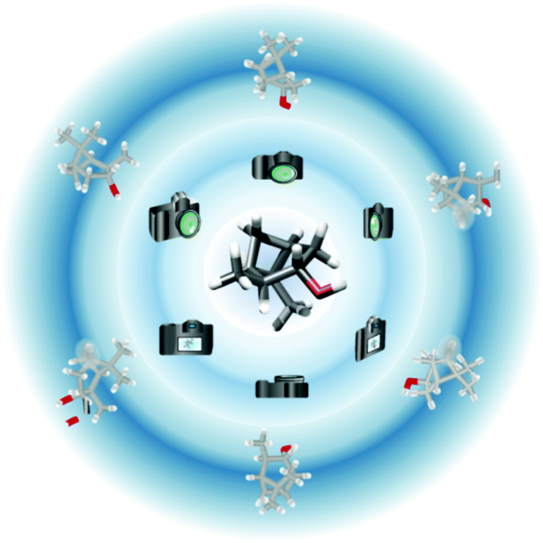Fig. 1 By measuring (camera) RDCs in an alignment medium (perspective), a projection (outer structures) of the molecule can be obtained. This result itself does not contain all 3D structural information needed. If five (or more) sufficiently different (linearly independent) projections are combined, the 3D structure (central structure) can be reconstructed and its dynamics determined. Non-measurable RDCs lead to missing information (shadows on the projections), which complicate the reconstruction.

The drawback of this approach is the need of a good estimation of the alignment parameters. This can be mitigated by performing the MFA in an iterative fashion as suggested in the SCRM and ORIUM protocols.^18,20 This allows to utilize the full advantage of the MFA, which is the computation of structural and dynamical information from the RDCs simultaneously, without relying on a well-defined structure proposal at the beginning of the structure elucidation process. Only the connectivity needs to be known.^20,21

Recently, we introduced the software TITANIA (TITANIA performs iterative analysis of independent alignments),²¹ which enables MFA in the field of NMR spectroscopy of small organic compounds for the first time. The software uses only connectivity information of a small organic compound as a starting point and RDCs in at least five (linearly independent) alignment media to obtain information on the structure and dynamics from experimental RDC data in an iterative algorithm. TITANIA performs a detailed analysis of the provided data (e.g. by the self-consistency of dipolar couplings analysis, SECONDA)²² to give a measure on the linear independence and heterogeneous effects (for example differences in the dynamics between alignment conditions or experimental uncertainties) on the RDCs. The main algorithm is structured in three major steps, starting with the determination of the alignment parameters based on the current structure model (see eqn (1)). The results are then used to determine the spherical harmonics (see eqn (2)). From here a new model is generated and used to restart the cycle. Without setting at least one stereogenic centre to a fixed absolute configuration, the structure optimisation converges to either of the two possible enantiomers as – similar to other NMR methods – RDCs alone are generally not directly relatable to a specific enantiomer and only the relative configuration of the correct diastereoisomer can be obtained.²³

We demonstrated in our previous work²¹ that the relative configuration of small organic compounds can be successfully determined using simulated RDCs derived from experimental orientation parameters. For this we analysed the trajectories of chiral volumes,²⁴ order parameters and Monte-Carlo statistics for several combinations of small organic compounds, alignment conditions and RDC spin pairs. In addition, random Gaussian error was added to simulate the applicability of TITANIA under practical conditions. We were able to show that it was not necessary to define stereo information of any kind as the starting point of the optimization within TITANIA. The principal challenge we found in the previous study was the reliance on a sufficient number of RDCs from linearly independent alignment conditions. If this condition is not met, the MFA does not yield a unique solution. Fortunately, new alignment media^25–33 allow the measurement of potentially different alignments of the same molecule in different (co-)solvents or, for example, at different temperatures. Additionally, modern pulse sequences,^34–44 developed in recent years, have simplified access to long-range RDCs. While we focus mainly on ⁿD_HH RDCs,^42,43 any additional long-range RDCs improve the sampling of vector orientations contributed by each individual RDC data set. This progress has now made it possible to obtain sufficiently large and different experimental RDC data sets and apply the MFA to small organic compounds as demonstrated here for the first time.

Even with all these improvements however, experimental spectra do not always give access to all theoretically possible couplings. This is typically the case due to broadened lines (elicited by the large number of dipolar couplings), strong or too large coupling (if a too high degree of orientation is present) or simply obfuscation by spectral overlap. These inaccessible RDCs lead either to the reduction of the total data set, since the corresponding rows (RDC vectors) or columns (alignment media) have to be removed from the RDC matrix, or to undefined elements in this very matrix. In such a case, the presented matrix eqn (1) and (2) cannot be applied without further modification. If such undefined RDCs would be set to 0.0 Hz, this would introduce wrong structure or dynamics information in the analysis (see ESI†).

Here we present two approaches that reduce the impact of undefined RDCs (voids in D) in the MFA. These are called recalculation and weighting scheme, respectively. The recalculation scheme takes advantage of the iterative nature of TITANIA. In each iteration step a refined structure is generated, on the basis of which the eqn (1) and (2) are solved. Thus, at the beginning of every iteration, undefined RDCs are back-calculated. The weighting scheme decomposes the matrix equations into vector equations. Thereby only one alignment medium (adjusted eqn (1)) and RDC vector (adjusted eqn (2)), respectively, is considered at a time. In this scheme, the undefined RDCs are removed from the equations by weighting factors prior to SVD (for more information see ESI†).

By back-calculating the RDCs the TITANIA optimization is expected to proceed more slowly, since structural errors affect not only the current iteration, but also each subsequent step. On the other hand, if RDCs are removed, especially if the number of alignment media is small, errors due to the reduction of matrix rank in the formation of pseudoinverses by SVD have to be expected. This data reduction is in competition with the requirement of linear independence of the orientations, which may be more challenging to achieve for small organic compounds due to the intrinsically smaller amount of data as compared to biomacromolecules. For a more detailed description of the algorithms, please refer to Chapter 1 of the ESI.†

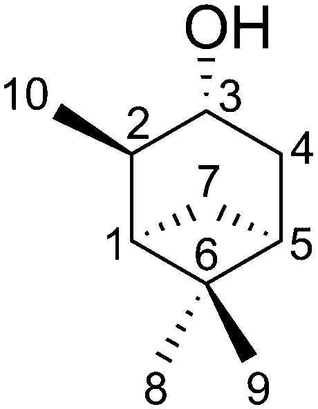
The applicability of TITANIA, also regarding the problem of missing elements in the RDC matrix, will be demonstrated on the NMR spectroscopically well studied compound isopinocampheol 1 (IPC). For this purpose, we measured 38 RDCs (11 ¹D_CH^37,39 or derived ¹D_CC⁴⁵ and 27 long-range ⁿD_HH⁴² RDCs) in six alignment conditions^29,46,47 (hereafter called set). This results in an RDC matrix with up to 228 elements, with a total of 23 undefined RDCs. To investigate the influence of the latter, four RDC setups were generated from the described matrix. These have different amounts and clusters of undefined RDCs. The process of generating the setups is described in the ESI† (see Chapter 7). Setup A-6 uses all 38 RDCs per set with 23 undefined elements (228 RDCs/10.0%). B-6 with a maximum of 33 RDCs per set and a total of 12 undefined elements (198 RDCs/6.1%) was generated by removing as many RDCs with multiple undefined elements as possible. C-6 with a maximum of 28 RDCs per set and 8 undefined elements (168 RDCs/4.8%) was created by having as few undefined elements per set as possible. The completely reduced setup D-6 with 24 RDCs per set has no undefined elements (144 RDCs/0.0%). The assignment of the media and RDC pairs can be found in the ESI.†

Using the simulated RDC data for isopinocampheol in our previous work²¹ showed that 11 ¹D_CH RDCs per set alone were not always sufficient to reliably determine the relative configuration, especially when considering Gaussian errors in the RDC data. While there may be less-challenging cases where readily accessible ¹D_CH RDCs are sufficient to reliably converge to the correct relative configuration, we found that the addition of 6 long-range ⁿD_HH RDCs per set significantly improved the reliability of the structure optimisation for IPC, which generally further improved with more long-range RDC data. This may serve as an estimate of the least amount of RDC data required for successful application of TITANIA but is certainly strongly dependent on the complexity of the compound investigated and its dynamics. The experimental RDC datasets for IPC analysed herein are similar in matrix size to the simulated data used previously, but are incomplete and additionally may exhibit heterogeneous behaviour due to the experimental uncertainties.

First, the setups A–D are analysed using SECONDA,²² which is used in biomolecular NMR spectroscopy to analyse heterogeneities between RDC datasets. In addition, as a principal component analysis (PCA), SECONDA collates information on the linear independence of the RDC datasets. As discussed above, SECONDA is also sensitive to voids in the RDC matrix, requiring data reduction or back-calculation²² or adjustments to the underlying equations. The adjustments we made and the resulting data are summarized in the ESI.† The key result of the SECONDA analysis is that the data sets contain at least three strongly different (linearly independent) orientations. This is especially clear when looking at the cumulative sum of the principle variances. For all setups, the largest three principle variances (λ₁–λ₃) represent >98% of the total variance. The following two principle variances (λ₄ and λ₅) are greater than 0.1. Thus, mathematically, a rank of 5 is always achieved. As a result of the analysis, the optimization of the rigid molecule IPC should succeed when using the four RDC setups within TITANIA.

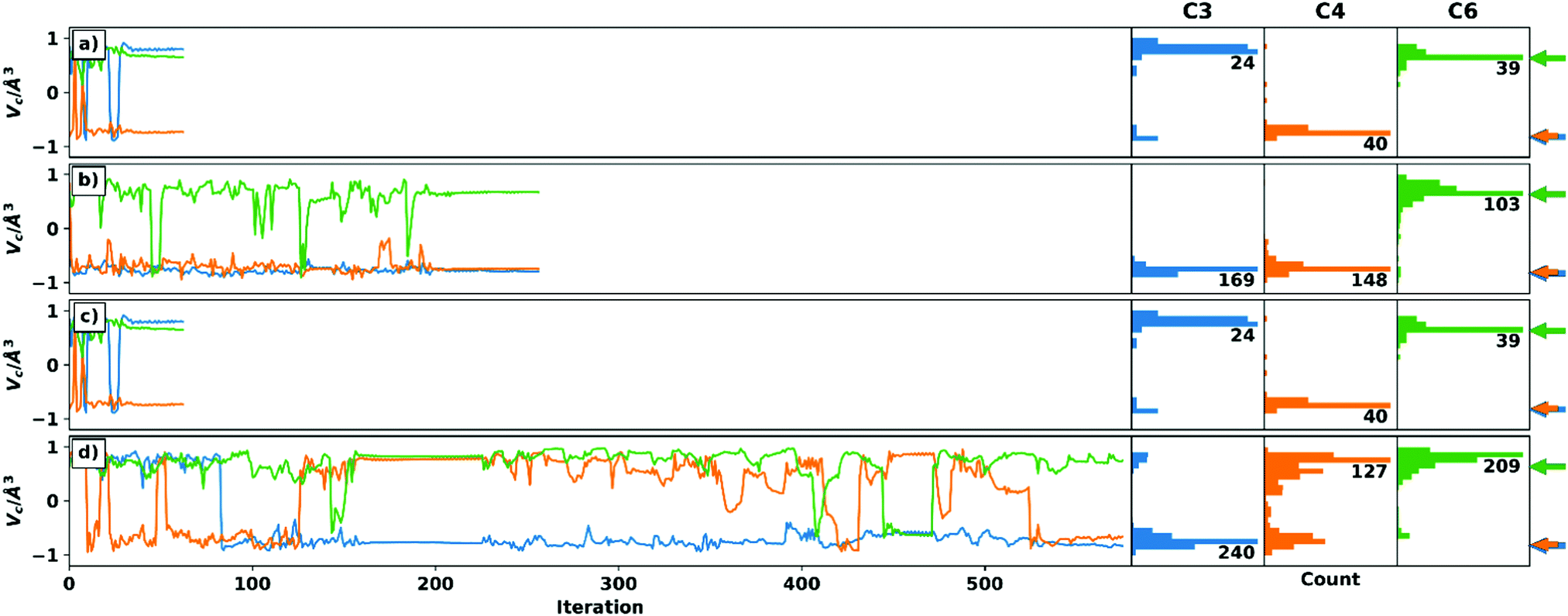
Four optimizations are performed for each setup, which differ in the choice of the algorithm for handling the voids and the choice of the starting structure. Thus, both schemes were started from the C3 epimer to ensure comparability of the optimizations. In addition, a randomly generated geometry was used. While the convergence criteria are set to identical values (see ESI† for details on the simulation setup), they are expected to be reached at different iteration steps for the different starting geometries and RDC data sets. The trajectories of the chiral volumes of the three centres C4 (two ¹D_CH RDCs), C3 (one ¹D_CH RDC), and C6 (two ¹D_CC RDCs) in the course of the optimizations of setup A-6 (23 undefined/228 total RDCs) are shown in Fig. 2, where the distributions of the chiral volumes are shown as a histogram on the y-axis. As noted above, RDC analysis in general is only able to yield relative configurations²³ and the given absolute configuration is a mathematical artefact of the starting geometry. For display purposes, we have decided to show the calculation results directly and indicate the expected relative chiral volume for the given configuration in each case individually by the coloured arrows at the right side of the histograms. For an example of a run converging to the enantiomeric absolute configuration (based on the distribution shown in the histograms) see panel c.

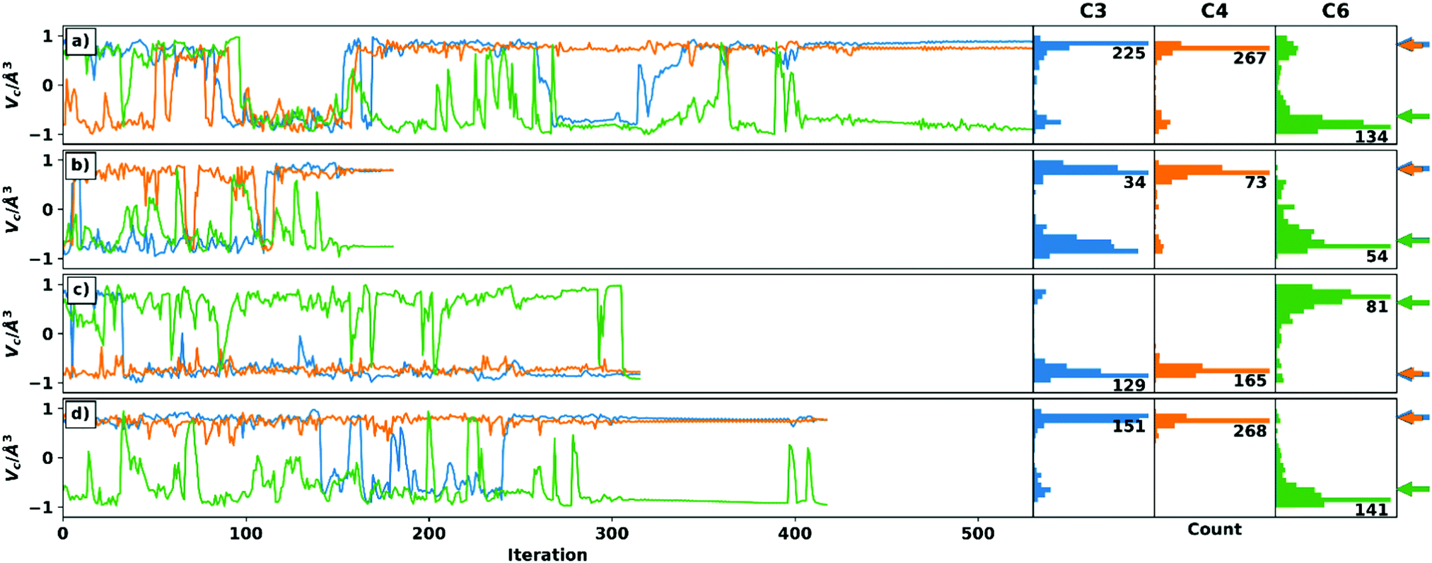Fig. 2 Trajectories of the chiral volumes of setup A-6 (all RDC data, 23 undefined elements) using the weighting scheme (panel a/b) and the recalculation scheme (panel c/d), respectively. For better comparability, the C3 epimer was used as the starting structure in panel a/c. The starting structures in panel b/d were chosen randomly. The arrows (blue and orange are almost identical) on the right side show the correct chiral volumes (which cannot be translated directly to the absolute configuration of the centres (see text)) of the respective enantiomer obtained. Only C6 in panel c has the incorrect relative configuration in the final structure. It can be assigned correctly by statistical analysis of the distribution of chiral volumes shown as histograms on the right.

Panels a and d show how most trajectories are expected to progress: many inversion steps sample the relevant geometries during the initial stages with only a few changes quickly reverting to the stable configuration in the latter stages, once convergence of the full trajectory is reached. With only two exceptions, the relative configuration of the centres can be unambiguously determined when considering the final structure and the distribution of the chiral volumes.

The first exception is C6 in the recalculation scheme with C3 epimer as starting structure (green line in panel c). Here, just before reaching convergence, centre C6 is inverted to the wrong configuration. The statistical distribution, on the other hand, shows the correct relative configuration. In the Cartesian coordinates, the final structure has no reasonable geometry at the corresponding centre. Due to the small number and magnitude of RDCs at a quaternary centre, its correct configuration is sometimes difficult to determine in TITANIA optimizations. For the case described here, however, an interchange of the C6–C8 and C6–C9 bond vectors would have little effect on the structure determination, since these are diastereotopic methyl groups.

The second exception is C3 in the weighting scheme with random starting structure (blue line in panel b). Here, the final structure is stable in the correct relative configuration. The distribution, on the other hand, does not show a single maximum as would be expected (a more detailed discussion is given in the ESI†). However, when examining the Cartesian coordinates’ trajectory, it becomes obvious that C3 is much more stable in the final structure, while the incorrect, early structures show a distorted geometry. The ambiguous distribution thus arises from the comparatively fast convergence which complicates the statistical evaluation of the chiral volume distribution.

Fig. 2 shows that TITANIA can handle undefined elements in the experimental RDC matrix for both schemes. Chiral centres involved in multiple RDCs (e.g. C4) show very narrow distributions in all cases and a very stable chiral volume in late iterations. This stability decreases with lower numbers of RDCs. The discussed ambiguities can be identified and interpreted by close inspection of the Cartesian coordinates. Additional indications for incorrect solutions are bond lengths that deviate strongly from literature data (vide infra) or inconsistent configurations when starting from different structures. Thus, changing the starting structure for inconclusive runs is a tool for confirming relative configurations.

In addition to the previously discussed trajectories of setup A-6, the chiral volume trajectories and Monte-Carlo data of all other setups are given in the ESI.† The optimization of setups with undefined elements in the RDC matrix should be accompanied by the statistical consideration of the Cartesian coordinate trajectories for reliable structure elucidation. The weighting scheme is superior to the recalculation scheme, especially for smaller data sets with voids (B-6 and C-6, see ESI†).

Additionally, the setup with the smallest data set (D-6) but without undefined elements will be discussed here (see Fig. 4): The optimizations with setup D-6 were performed using both schemes, although there are no voids in the RDC data set. On the one hand, it can be shown that panels a and c have the same trajectory, since the same starting structure was used. Thus, the choice of the different schemes has no effect for complete datasets. On the other hand, setup D-6 shows the possibility of confirming configurations by changing the starting structure (panel b and d). This has proven to be important for C3 and C4. Centre C4 shows an ambiguous assignment in panel d based on the distribution of chiral volumes. The reason for this is the late inversion to the correct configuration, which can be detected by checking the Cartesian coordinates as described above.

Similarly, the wrong configuration of C3 in the identical trajectories of panels a and c can be detected by the distorted bond lengths at C3 and the neighbouring carbons C2 and C4 of the final structure. For example, the bond length r_C3H3 = 0.82 Å is exceptionally short, which is typical for stereogenic centres in the wrong configuration. In addition, the bonds vicinal to this are also significantly elongated with r_C2H2 = 1.24 Å and r_C4H4a = 1.29 Å. The reason for this becomes clear when assessing the final (left) and reference structure (right) in Fig. 3. The aforementioned bonds (red arrows) are shortened or lengthened to optimize the RDC vectors (blue arrows) to fit better to the actual orientation (green arrows). These distorted geometries for wrongly configured stereogenic centres are often elicited by the inverse vector solution.²¹ In this special case, however, it is the result of too fast convergence. In the ESI,† two additional trajectories are shown, in which either the weighting of the bond lengths was reduced by a factor of 5 or the number of iteration steps was increased by more stringent convergence criteria. Both options lead to the correct configuration at all centres.

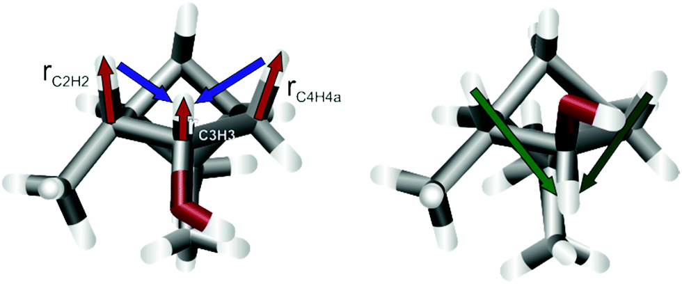Fig. 3 Final structure of D-6 starting from epi-C3 (left) and the reference structure from literature.⁴⁶ The red arrows show the bond lengths, that are distorted to compensate the difference in the long-range ⁿD_HH coupling vectors (blue and green). Starting the optimization from a different geometry, e.g. random coordinates, alleviates this problem.

Fig. 4 Trajectories of the chiral volumes of setup D-6 (reduced RDC data, no undefined elements) using the weighting scheme (panel a/b) and the recalculation scheme (panel c/d), respectively. For better comparability, the C3 epimer was used as the starting structure in panel a/c. The starting structures in panel b/d were chosen randomly. The arrows (blue and orange are almost identical) on the right side show the correct chiral volumes (which cannot be translated directly to the absolute configuration of the centres (see text)) of the respective enantiomer obtained. The panels a and c are identical, due to the fact that no RDCs are missing. The wrong configuration of C3 is discussed in the main text and ESI.†

Conclusions

With the presented data, we showed how TITANIA contributes new insights into the de novo structure determination of small organic compounds based entirely on experimental RDCs. In contrast to previous approaches the new quality of information, namely direct vector information, accessible from multiple alignment data sets was used to achieve this goal. In the discussed borderline cases that did not lead to the correct configuration of the final structures in the first try, these errors could be detected by assessing the geometry in detail or the statistical processing of the data. Here the correct structure was additionally obtained by changing the starting structure or adjusting the settings.

The selection of different alignment media used here is limited to polypeptide-based alignment media. While the alignments proved sufficiently linearly independent, we expect a further broadening of the applications when employing the full range of other recently developed alignment media.^5,25–33 Further improvements are expected upon the inclusion of more difficult to access long-range ⁿD_CH or ^1/nD_CC couplings. The use of additional complementary data is expected to significantly improve the determination of flexibility or reduce the influence of experimental errors and even missing RDCs. Moreover, additional couplings^34–44 would drastically simplify the determination of challenging centres (such as C6 in IPC).

Herein we were able to demonstrate the capability of TITANIA to determine the relative configuration of IPC using an incomplete, experimental RDC dataset. This revolutionizes the structure elucidation of small organic compounds. By the continuous developments of new (stimuli responsive)⁴⁷ alignment media and modern pulse sequences the full investigation of flexible molecules, including the determination and analysis of local order parameters, is currently under investigation.

Data availability

The source code for the TITANIA program is available at https://doi.org/10.5281/zenodo.5548105. Raw NMR spectra and TITANIA input and output files are available as supplementary material at https://doi.org/10.5281/zenodo.5636052

Conflicts of interest

There are no conflicts of interest to declare.

Notes and references

1. B. Böttcher and C. M. Thiele, Encyclopedia of Magnetic Resonance, 2012 DOI:10.1002/9780470034590.emrstm1194.
2. R. R. Gil, Angew. Chem., Int. Ed., 2011, 50, 7222–7224.
3. G. Kummerlöwe and B. Luy, in Annu. Rep. NMR Spectrosc., ed. G. A. Webb, Academic Press, 2009, vol. 68, pp. 193–232.
4. J. A. Losonczi, M. Andrec, M. W. F. Fischer and J. H. Prestegard, J. Magn. Reson., 1999, 138, 334–342.
5. V. Schmidts, Magn. Reson. Chem., 2017, 55, 54–60.
6. F. Kramer, M. V. Deshmukh, H. Kessler and S. J. Glaser, Conc. Magn. Reson. A, 2004, 21A, 10–21.
7. J. R. Tolman, J. Am. Chem. Soc., 2002, 124, 12020–12030.
8. G. Cornilescu, J. L. Marquardt, M. Ottiger and A. Bax, J. Am. Chem. Soc., 1998, 120, 6836–6837.
9. D. Ban, T. M. Sabo, C. Griesinger and D. Lee, Molecules, 2013, 18, 11904–11937.
10. K. Chen and N. Tjandra, Top. Curr. Chem., 2012, 326, 47–67.
11. G. Cornilescu, R. F. Ramos Alvarenga, T. P. Wyche, T. S. Bugni, R. R. Gil, C. C. Cornilescu, W. M. Westler, J. L. Markley and C. D. Schwieters, ACS Chem. Biol., 2017, 12, 2157–2163.
12. S. Immel, M. Köck and M. Reggelin, Chem. – Eur. J., 2018, 24, 13918–13930.
13. P. Tzvetkova, U. Sternberg, T. Gloge, A. Navarro-Vázquez and B. Luy, Chem. Sci., 2019, 10, 8774–8791.
14. G. Lipari and A. Szabo, J. Am. Chem. Soc., 1982, 104, 4546–4559.
15. G. Lipari and A. Szabo, J. Am. Chem. Soc., 1982, 104, 4559–4570.
16. J. Meiler, J. J. Prompers, W. Peti, C. Griesinger and R. Brüschweiler, J. Am. Chem. Soc., 2001, 123, 6098–6107.
17. W. Peti, J. Meiler, R. Brüschweiler and C. Griesinger, J. Am. Chem. Soc., 2002, 124, 5822–5833.
18. N.-A. Lakomek, K. F. A. Walter, C. Farès, O. F. Lange, B. L. de Groot, H. Grubmüller, R. Brüschweiler, A. Munk, S. Becker, J. Meiler and C. Griesinger, J. Biomol. NMR, 2008, 41, 139.
19. N. R. Skrynnikov, N. K. Goto, D. Yang, W.-Y. Choy, J. R. Tolman, G. A. Mueller and L. E. Kay, J. Mol. Biol., 2000, 295, 1265–1273.
20. T. M. Sabo, C. A. Smith, D. Ban, A. Mazur, D. Lee and C. Griesinger, J. Biomol. NMR, 2014, 58, 287–301.
21. F. A. Roth, V. Schmidts and C. M. Thiele, J. Org. Chem., 2021, 86, 15387–15402.
22. J.-C. Hus, W. Peti, C. Griesinger and R. Brüschweiler, J. Am. Chem. Soc., 2003, 125, 5596–5597.
23. R. Berger, J. Courtieu, R. R. Gil, C. Griesinger, M. Köck, P. Lesot, B. Luy, D. Merlet, A. Navarro-Vázquez, M. Reggelin, U. M. Reinscheid, C. M. Thiele and M. Zweckstetter, Angew. Chem., Int. Ed., 2012, 51, 8388–8391.
24. T. F. Havel, I. D. Kuntz and G. M. Crippen, Bull. Math. Biol., 1983, 45, 665–720.
25. A. Marx, B. Böttcher and C. M. Thiele, Chem. – Eur. J., 2010, 16, 1656–1663.
26. N.-C. Meyer, A. Krupp, V. Schmidts, C. M. Thiele and M. Reggelin, Angew. Chem., Int. Ed., 2012, 51, 8334–8338.
27. C. Merle, G. Kummerlöwe, J. C. Freudenberger, F. Halbach, W. Stöwer, C. L. V. Gostomski, J. Höpfner, T. Beskers, M. Wilhelm and B. Luy, Angew. Chem., Int. Ed., 2013, 52, 10309–10312.
28. X. Lei, Z. Xu, H. Sun, S. Wang, C. Griesinger, L. Peng, C. Gao and R. X. Tan, J. Am. Chem. Soc., 2014, 136, 11280–11283.
29. S. Jeziorowski and C. M. Thiele, Chem. – Eur. J., 2018, 24, 15631–15637.
30. M. Schwab, V. Schmidts and C. M. Thiele, Chem. – Eur. J., 2018, 24, 14373–14377.
31. M. Schwab, D. Herold and C. M. Thiele, Chem. – Eur. J., 2017, 23, 14576–14584.
32. L. F. Gil-Silva, R. Santamaría-Fernández, A. Navarro-Vázquez and R. R. Gil, Chem. – Eur. J., 2016, 22, 472–476.
33. M. Reller, S. Wesp, M. R. M. Koos, M. Reggelin and B. Luy, Chem. – Eur. J., 2017, 23, 13351–13359.
34. M. Kurz, P. Schmieder and H. Kessler, Angew. Chem., Int. Ed. Engl., 1991, 30, 1329–1331.
35. D. Uhrín, G. Batta, V. J. Hruby, P. N. Barlow and K. E. Kövér, J. Magn. Reson., 1998, 130, 155–161.
36. A. Meissner and O. W. Sørensen, Magn. Reson. Chem., 2001, 39, 49–52.
37. K. Fehér, S. Berger and K. E. Kövér, J. Magn. Reson., 2003, 163, 340–346.
38. K. E. Kövér and K. Fehér, J. Magn. Reson., 2004, 168, 307–313.
39. A. Enthart, J. C. Freudenberger, J. Furrer, H. Kessler and B. Luy, J. Magn. Reson., 2008, 192, 314–322.
40. C. M. Thiele and W. Bermel, J. Magn. Reson., 2012, 216, 134–143.
41. L. Castañar, J. Sauri, R. T. Williamson, A. Virgili and T. Parella, Angew. Chem., Int. Ed., 2014, 53, 8379–8382.
42. D. Sinnaeve, J. Ilgen, M. E. Di Pietro, J. J. Primozic, V. Schmidts, C. M. Thiele and B. Luy, Angew. Chem., Int. Ed., 2020, 59, 5316–5320.
43. D. Sinnaeve, M. Foroozandeh, M. Nilsson and G. A. Morris, Angew. Chem., Int. Ed., 2016, 55, 1090–1093.
44. W. Koźmiński and D. Nanz, J. Magn. Reson., 2000, 142, 294–299.
45. L. Verdier, P. Sakhaii, M. Zweckstetter and C. Griesinger, J. Magn. Reson., 2003, 163, 353–359.
46. A. Marx, V. Schmidts and C. M. Thiele, Magn. Reson. Chem., 2009, 47, 734–740.
47. M. Hirschmann, D. S. Schirra and C. M. Thiele, Macromolecules, 2021, 54, 1648–1656.

---

Footnote

† Electronic supplementary information (ESI) available: One pdf file containing all runs and their discussion. See DOI: 10.1039/d1cp02324a

---