Self-learning entropic population annealing for interpretable materials design

Abstract

In automatic materials design, samples obtained from black-box optimization offer an attractive opportunity for scientists to gain new knowledge. Statistical analyses of the samples are often conducted, e.g., to discover key descriptors. Since most black-box optimization algorithms are biased samplers, post hoc analyses may result in misleading conclusions. To cope with the problem, we propose a new method called self-learning entropic population annealing (SLEPA) that combines entropic sampling and a surrogate machine learning model. Samples of SLEPA come with weights to estimate the joint distribution of the target property and a descriptor of interest correctly. In short peptide design, SLEPA was compared with pure black-box optimization in estimating the residue distributions at multiple thresholds of the target property. While black-box optimization was better at the tail of the target property, SLEPA was better for a wide range of thresholds. Our result shows how to reconcile statistical consistency with efficient optimization in materials discovery.

---

Introduction

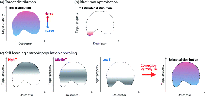
Automatic design of materials based on black-box optimization¹ has shown tremendous success in developing functional materials including organic chemical compounds,² inorganic materials³ and biopolymers such as peptides⁴ and proteins.² Popular methods of black-box optimization include Bayesian optimization,⁵ and evolutionary algorithms.^6,7 Given a candidate material, an experiment is regarded as a black-box function that returns its property value such as bioactivity,⁸ thermal conductivity⁹ or electron gain energy.¹⁰ Black-box optimization is an iterative procedure that recommends one material or a batch of materials for experiments at a time. It is expected to find a material with a favorable property with a minimum number of experiments. Notice that an experiment is often replaced with a simulator or a prediction model.

Samples obtained from black-box optimization offer an attractive opportunity for scientists to gain new knowledge. Statistical analyses of the samples are often conducted to discover new structure–property relationships,¹⁰ or key descriptors that explain their favorable property.¹¹ However, such analyses have to be done with caution, because most of the existing black-box optimizers are biased samplers. Fig. 1a and b show a schematic picture about this issue. This paper aims to develop algorithmic methods that achieve efficient optimization and statistical consistency at the same time.

Fig. 1 Estimation of the joint distribution of the target property and a descriptor of interest. (a) Ground-truth distribution derived from all possible materials. (b) Black-box optimization creates a number of samples, but simply plotting them leads to a misleading picture. (c) In self-learning entropic population annealing, samples are obtained at multiple temperatures. They are integrated with weights to yield an accurate estimation of the whole distribution.

Density-of-states (DoS) refers to the probability distribution of observables of a physical system such as spin glass.¹² Observables may include energy, pressure and other physical parameters. If DoS is obtained, the free energy of the target physical system can be evaluated and the system is regarded as understood. Exact estimation of DoS requires enumeration of all possible physical configurations which involves prohibitive computational cost. Estimation of DoS is nevertheless possible with sampling methods including the Wang–Landau method¹³ and stochastic approximation Monte Carlo.¹⁴ These methods are known under the umbrella term entropic sampling. They have mechanisms to obtain samples from low energy regions, which are hardly found by naive sampling procedures due to the small occurrence probability. In this paper, we use entropic sampling in the context of interpretable materials design. The target property and a descriptor are designated as the energy of the system and an additional observable, respectively, and the joint distribution is estimated as DoS.

Among several methods of entropic sampling, we employ entropic population annealing (EPA)¹⁵ as our base method, and extend it to self-learning EPA (SLEPA) by incorporating a machine learning model. In both methods, Boltzmann distributions at multiple temperatures are introduced and some samples are obtained from each distribution using Markov chain Monte Carlo (MCMC) (Fig. 1c). As the temperature is decreased, the samples are gradually concentrated towards optimal solutions. Then, DoS is estimated from the samples using the multiple histogram method (MHM).¹⁶ The difference between EPA and SLEPA is that EPA accesses the energy (i.e., target property) whenever a new sample is created, while SLEPA uses a predicted value from the surrogate machine learning model. SLEPA tends to be more cost effective, but the distribution shift made by the prediction error has to be corrected eventually in DoS estimation.

In computational experiments, SLEPA and EPA were evaluated in a peptide design problem, where scientists are interested in finding sequential signatures that determine the properties.¹⁷ We are thus committed to estimating the residue distributions of qualified sequences that correspond to a small percentile in the target property. Multiple qualification thresholds ranging from 0.01 to 10 percentiles were used. When an evolution strategy (ES),⁶ a pure black-box optimizer, was applied, its estimation accuracy was best for the tightest thresholds. Simple random sampling was best for the loosest thresholds. For a wide range of thresholds, however, SLEPA and EPA were better than them. SLEPA showed better estimation accuracies than EPA, indicating that the use of a surrogate model enhances sample efficiency. This result illustrates how to reconcile statistical consistency with efficient optimization and shows the usefulness of our approach when acquiring knowledge is more important than optimization.

Method

Observables and density of states

Let X denote the set of all possible materials. In black-box optimization, we aim to find x ∈ X that minimizes the target property e(x). Obtaining e(x) for x incurs certain cost, because it is done via an experiment or numerical simulation. In the following, e(x) is referred to as energy and the acquisition of e(x) is called observation. In this paper, we deal with the research tasks where the relationship between e(x) and d(x), a descriptor, is of interest. More specifically, we need to find the expectation value of an observable O(d(x), e(x)), i.e., a function depending on e(x) and d(x),

The observable is determined according to users' interest. Let us suppose that one is interested in the descriptor value to yield a favorable target property, e(x) ≤ δ, where δ is a qualification threshold. The observable should then be set as O(d(x), e(x)) = d(x)I(e(x) ≤ δ), where I(·) is the indicator function which is one if the condition in the parentheses is satisfied, zero otherwise. Also, if one needs to draw a two dimensional distribution as in Fig. 1, the density at the grid e_l ≤ e(x) ≤ e_h, d_l ≤ d(x) ≤ d_h can be obtained by setting O(d(x), e(x)) = I(d_l ≤ d(x) ≤ d_h, e_l ≤ e(x) ≤ e_h).

In understanding our method, it is beneficial to reformulate 〈O〉 from another viewpoint, i.e., histogram-based view. Let E and D denote all possible values of e(x) and d(x), respectively. The observable expectation of eqn (1) can be rewritten as

whereis called density of states (DoS) with respect to e and d. The DoS n(e) of target property e(x) without considering the descriptor d(x) can be defined in a similar way.

Multicanonical sampling

In multicanonical sampling,¹² we consider a family of distributions parameterized by inverse temperature β,

P_β(x) = exp(−βe(x) + f), (4)

where f corresponds to the normalization factor,called free energy. Let us assume that N_i samples {x_ij}_j=1,…,Ni at inverse temperature β_i (i = 1, …, τ) are obtained using a sampling technique. Here, τ is the number of inverse temperature. To generate {x_ij}_j=1,…,Ni, there are several possible techniques, but we employ PA¹⁸ as detailed in the next subsection. Using the samples, the observable is estimated aswhere r_i(e) denotes non-negative weight parameters, , and f_i is the normalization factor at β_i. The weights are determined so that the estimation error of DoS with respect to e, n(e), is minimized.¹⁶ By using MHM which will be explained later, r_i(e) and n(e) are estimated. A consistent estimate of 〈O〉 can be obtained via correction by weights r_i(e) (see Fig. 1c).

Population annealing

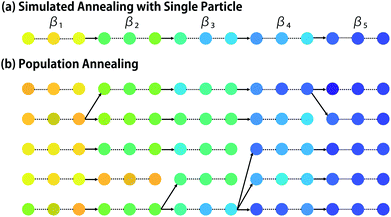
Population annealing (PA) was developed by Hukushima and Iba¹⁹ as an improved form of simulated annealing.²⁰ In recent years, it has been applied to various problems in physics.^21,22 In the simplest form of simulated annealing, an initial particle x is randomly chosen, and the increasing sequence of β = β₁, …, β_τ is given (see Fig. 2a). Hereinafter, the maximum and minimum inverse temperatures are denoted as β_max = β_τ and β_min = β₁, respectively. At the i-th iteration, K_i samples by P_βi(x) are generated by applying the MCMC method. One can apply any MCMC method including Metropolis sampling and Gibbs sampling.¹² When Metropolis sampling is employed, particle x is randomly perturbed to x′ and it is accepted with probability min(1, P_β(x′)/P_β(x)). If rejected, the particle stays the same. In population annealing, M particles {x_m}_m=1,…,M are used. At i-th iteration, K_i samples by P_βi(x) are generated for each particle by MCMC steps with fixed β_i, and N_i = M × K_i. Then, the particles are resampled to fit to the next canonical distribution P_βi+1(x). In this resampling, the probability for x_m is determined as

q_m ∝ exp(−(β_i+1 − β_i)e(x_m)). (7)

Fig. 2 Simulated annealing and population annealing towards minimization of the target property. Each dot represents a particle and its color corresponds to the property value. (a) Simulated annealing achieves minimization via MCMC sampling with gradually increasing inverse temperature β. (b) Population annealing retains multiple particles. When the temperature changes, resampling is performed for adjustment to the new temperature. Some particles multiply, while others vanish.

The particle set is updated by drawing M particles with replacement. As a result, a particle may vanish or multiply (see Fig. 2). Reweighting is similar to natural selection in evolution algorithm,⁷ because poor particles with high e are more likely to vanish. It is known that, when the temperature difference |β_i+1 − β_i| is too large, resampling may lead to loss of diversity, i.e., all particles end up having the same ancestor.²³

Multiple histogram method

MHM is a numerical algorithm for estimating the DoS from the samples of Boltzmann distributions at multiple temperatures.¹⁶ Let us assume that N_i samples are obtained at temperature β_i by PA, and denote the number of samples with energy e as h_i(e). In MHM, using weight parameters r_i(e), DoS is obtained aswhere p_i(e) is the Boltzmann distribution at temperature β_i, and f_i is the free energy described as

The weights r_i(e) are determined to minimize the estimation error of n(e). MHM assumes that h_i(e) is subject to Poisson distribution whose mean is N_in(e)exp(−β_ie + f_i). Since the variance of a Poisson distribution is equal to its mean, the variance of h_i(e) is described as V[h_i(e)] = N_in(e)exp(−β_ie + f_i). So the variance of p_i(e) ≈ h_i(e)/N_i is derived as

Due to the statistical independence of samples at different temperatures, we obtain the estimation error of n(e), i.e., the variance of n(e) as

The optimization problem for the weights r_i(e) is then defined as

Using a Lagrange multiplier, we obtain

Substituting it to eqn (8), we obtain the optimized representation of n(e),

The DoS n(e) and free energy f_i are obtained by solving the nonlinear system consisting of eqn (14) and (9) by fixed point iteration. When f_i is obtained, r_i(e) and 〈O〉 can be estimated.

Self-learning entropic population annealing

Like EPA, self-learning entropic population annealing (SLEPA) uses M particles and alternates MCMC steps and resampling. The difference is that the energy e(x) is replaced by the prediction by a machine learning model ẽ_i(x) (see Fig. 3). In our experiments, we used Gaussian process regression²⁴ as the machine learning model. The model is updated as more and more training examples are available. The first model ẽ₁(x) is trained by initial M particles and their energies. The i-th model corresponding to β_i is trained by iM examples obtained up to the point. Notice that the number of MCMC steps K_i does not affect the number of observations in SLEPA. So K_i can be set to a reasonably large value to ensure the convergence of MCMC steps. Populations of samples obtained from SLEPA are based on the Boltzmann distributions of predicted energies. Before applying MHM, these populations are corrected by resampling. The weight of the j-th particle obtained at β_i is described as

q_ij ∝ exp[−β_i(e(x_ij) − ẽ_i(x_ij))]. (15)

Fig. 3 Flow of self-learning entropic population annealing (SLEPA). SLEPA alternates MCMC steps and resampling based on an energy function predicted by a machine learning algorithm. After all samples are obtained, the distribution shift made by prediction error is corrected via additional resampling. Finally, the DoS is derived from resampled populations.

Results

Estimation of residue distribution

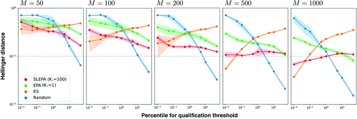
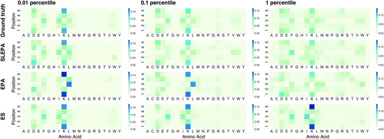
To illustrate how SLEPA can be used in practice, short peptides of length five are designed. Recently, antimicrobial peptides have been of increasing interest to address the threat of multidrug-resistant pathogens.¹⁷ Strong hydrophobic moment²⁵ is a distinct feature of antimicrobial peptides.¹⁷ Motivated by this fact, the target property e(x) is designated as hydrophobic moment which is computed using a prediction model implemented in python library modlAMP.¹⁷ Given a budget on the number of observations, our goal is to estimate the residue distribution for qualified sequences e(x) ≤ δ, where δ is a qualification threshold. In SLEPA and EPA, the number of iterations is set to τ = 20, and the inverse temperatures are set between β_min = 0 and β_max = 10 with equal interval. In an MCMC step, a residue at a randomly chosen position is changed to a random residue (i.e., one residue flip). The number of MCMC steps of SLEPA is determined as K_i = 100, while that of EPA is set to one to save the number of observations. As the surrogate model of SLEPA, we use Gaussian process regression implemented in PHYSBO.²⁴ To train the surrogate model, each residue is encoded to a seven dimensional feature vector called Tscale.²⁶ As baselines, we employ simple random sampling and (μ, λ) evolution strategy (ES).⁶ In the ES, λ particles are retained. In each step, the energies of all particles are observed and top μ particles are chosen. A new generation of λ particles are generated by applying one residue flip to the chosen ones. The number of particles λ and the number of iterations are aligned with SLEPA and EPA, and μ is fixed to 10% of λ. For simple random sampling and ES, the residue distribution is constructed by counting.

Fig. 4 shows the Hellinger distance of the residue distribution obtained by each method to the ground truth distribution obtained by complete enumeration. The Hellinger distance is defined as the Euclidean distance of square roots of probabilities. It is robust against zero probabilities. In all methods, the distance gets smaller as the number of particles M is increased. In all ranges of M, the performance of ES, one of our baseline methods, deteriorates as the qualification threshold is relaxed. This is intelligible, because ES performs pure optimization and does not have a mechanism to keep statistical consistency. Simple random sampling, on the other hand, performs poorly when the qualification threshold is small due to lack of any optimization mechanism. SLEPA and EPA show stably good results at all qualification thresholds, reflecting the fact that these methods are designed to optimize while maintaining statistical consistency. SLEPA exhibits better results than EPA in most cases. This result indicates that the use of machine learning is effective in increasing the number of MCMC steps to improve distribution estimation. The best distribution estimates (M = 200) by SLEPA, EPA, and ES are shown in Fig. 5.

Fig. 4 Hellinger distance of the residue distribution to the ground truth distribution against the qualification threshold when β_max = 10 and τ = 20. Each plot corresponds to a different number of particles M. In all plots, the solid line and shaded area indicate the mean and standard deviation of five runs, respectively.

Fig. 5 Residue distributions of qualified peptides obtained by complete enumeration (i.e., ground-truth), self-learning entropic population annealing (SLEPA), entropic population annealing (EPA), and evolution strategy (ES). For each method, the best estimate in terms of the Hellinger distance to the ground truth among five runs is shown. The number of particles is 200.

Quality of samples

Fig. 6a shows the best target property against the number of particles. In addition, Fig. 6b and c show the number of unique samples qualifying the threshold. While ES, a pure optimization algorithm, is the best, SLEPA shows a competitive performance when the number of particles is relatively large. EPA is clearly behind SLEPA, indicating that the surrogate model improves optimization substantially. To get an idea about sample diversity, Fig. 6d shows the ratio of the number of unique samples to the total number. The ratio of ES is particularly low, because the samples are concentrated around the optimal point and duplications are likely to happen. Comparing SLEPA and EPA, the ratio of SLEPA is much higher due to the difference in the number of MCMC steps. Since the samples of SLEPA are well mixed by MCMC, there is a smaller chance to create duplications.

Fig. 6 (a) Minimum value of the target property against the number of particles M. (b) and (c) Number of qualified samples at 0.01 and 0.1 percentiles. (d) Ratio of the number of unique samples to the total number.

Number of MCMC steps

So far, the number of MCMC steps of EPA was set to one to keep the number of observations equal. In Fig. 7, we compared SLEPA and EPA with the same number of MCMC steps. When the number of MCMC steps of EPA is increased to 100, it was better than SLEPA in terms of the accuracy in distribution estimation and the number of qualified samples. This result shows the advantage of EPA that it can always make use of the correct energy instead of the predicted one. Although EPA was not performing well under a budget on observations, it is still a viable choice, if observation can be done cost effectively with fast simulation or a certain prediction model. See the ESI† for experimental results with other parameter settings.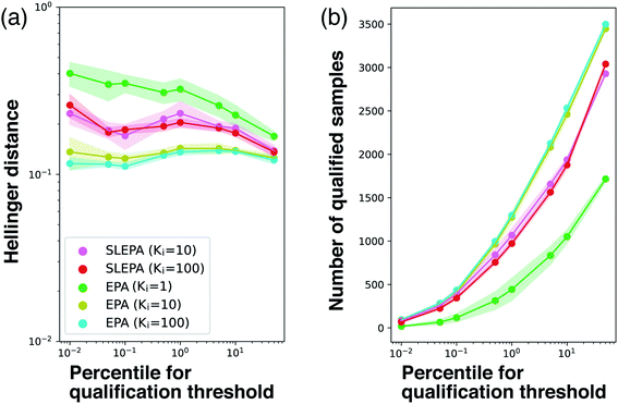

Fig. 7 (a) Hellinger distance to the ground truth distribution at M = 200. SLEPA (K_i = 10 and 100) and EPA (K_i = 1, 10, and 100) are compared. (b) Number of qualified samples.

Discussion

We have presented how automatic materials design can be made interpretable by introducing ideas from statistical physics and machine learning. In a benchmarking problem, it is confirmed that EPA and SLEPA have the desired property of accurate distribution estimation. So far, algorithmic methods for automatic materials design have been developed towards better optimization efficiency, paying minimum attention to statistical bias. Hopefully this paper sheds light on statistical consistency that is crucially important in correct understanding of materials.

In our experiments, SLEPA with a Gaussian process was better than EPA, but the performance of SLEPA depends on the choice of the surrogate model and its prediction ability. The use of a surrogate model can be disadvantageous in the occasions where the model works poorly.

While SLEPA can reveal correlations between variables, it is well known that correlation does not necessarily mean causation.²⁷ According to multiple studies, however, if the joint distribution satisfies certain criteria, it is possible to identify the causal direction from it.^28,29 The combination of SLEPA and such causal discovery methods may detect causal relationships among variables about materials properties.

The parameters of SLEPA consist of the number of MCMC steps K_i, the number of particles M, the inverse temperature array β_i and the hyperparameters of the adopted machine learning model. First of all, the number of MCMC steps should be set as large as possible to ensure the convergence in each iteration, but setting it over 1000 would be meaningless. For accurate DoS estimation, the number of particles M should be large too, but it is also affected by the capacity of the evaluator. For example, if SLEPA is used together with a simulator that can evaluate z materials in parallel, setting M to a value larger than z may result in unwanted latency. The inverse temperature array is determined first by setting the range [β_min, β_max] and dividing it into τ equally spaced points. As mentioned, a small τ leads to a large change of temperature that is harmful to resampling, while a large τ causes slow optimization. As in most black-box optimizers, we start from uniformly random samples, thus β_min = 0. Setting β_max would be the trickiest part, because, if too high, the probability is concentrated on one particle in almost all iterations and, if too low, the accuracy of DoS would be poor. To set β_max appropriately, we recommend computation of the unnormalized probability exp(−β_maxe(x)) for all initial examples to check if the probability is concentrated or scattered too much. Finally, the hyperparameters should be set according to the guideline of the machine learning model. In our experiments, we used the automatic hyperparameter initialization and update functions of PHYSBO.²⁴

The integration of statistical physics, machine learning, and materials design offers a great opportunity of algorithmic development. When SLEPA is applied in the latent space of variational autoencoders,² highly structural objects such as chemical compounds³⁰ and crystal structures³¹ can be generated. To solve multiobjective optimization problems, SLEPA can be extended to estimate multidimensional DoS.³² In addition, other entropic samplers such as replica-exchange Monte Carlo,¹⁸ broad histogram³³ and transition matrix Monte Carlo³⁴ may find their own advantages in the context of materials design.

Data availability

Additional experimental results are summarized in the ESI.† An implementation of SLEPA is available at https://github.com/tsudalab/SLEPA and https://doi.org/10.5281/zenodo.6339987. The code to reproduce the results in this paper is available at https://doi.org/10.5281/zenodo.6374926.

Author contributions

R. T. and K. T. conceived the idea and designed the research. All authors developed the algorithm, performed computational experiments, and wrote the manuscript.

Conflicts of interest

The authors declare no competing interests.

Acknowledgements

This work is supported by AMED JP20nk0101111, NEDO P15009, SIP (Technologies for Smart Bio-industry and Agriculture, “Materials Integration” for Revolutionary Design System of Structural Materials), JSPS Grant-in Aid for Scientific Research (Grant Number 21H01008), and JST ERATO JPMJER1903 and CREST JPMJCR21O2.

References

1. K. Terayama, M. Sumita, R. Tamura and K. Tsuda, Acc. Chem. Res., 2021, 54, 1334–1346.
2. B. Sanchez-Lengeling and A. Aspuru-Guzik, Science, 2018, 361, 360–365.
3. N. Szymanski, Y. Zeng, H. Huo, C. Bartel, H. Kim and G. Ceder, Mater. Horiz., 2021, 8, 2169–2198.
4. D. P. Tran, S. Tada, A. Yumoto, A. Kitao, Y. Ito, T. Uzawa and K. Tsuda, Sci. Rep., 2021, 11, 10630.
5. D. R. Jones, M. Schonlau and W. J. Welch, J. Glob. Optim., 1998, 13, 455–492.
6. I. Rechenberg, Comput. Methods Appl. Mech. Eng., 2000, 186, 125–140.
7. P. C. Jennings, S. Lysgaard, J. S. Hummelshøj, T. Vegge and T. Bligaard, npj Comput. Mater., 2019, 5, 1–6.
8. A. Zhavoronkov, Y. A. Ivanenkov, A. Aliper, M. S. Veselov, V. A. Aladinskiy, A. V. Aladinskaya, V. A. Terentiev, D. A. Polykovskiy, M. D. Kuznetsov and A. Asadulaev, et al. , Nat. Biotechnol., 2019, 37, 1038–1040.
9. S. Ju, T. Shiga, L. Feng, Z. Hou, K. Tsuda and J. Shiomi, Phys. Rev. X, 2017, 7, 021024.
10. Y. Zhang, J. Zhang, K. Suzuki, M. Sumita, K. Terayama, J. Li, Z. Mao, K. Tsuda and Y. Suzuki, Appl. Phys. Lett., 2021, 118, 223904.
11. H. Sahu, W. Rao, A. Troisi and H. Ma, Adv. Energy Mater., 2018, 8, 1801032.
12. K. Binder and D. W. Heermann, Monte Carlo simulation in statistical physics: an introduction, Springer, Heidelberg, 5th edn, 2010.
13. F. Wang and D. P. Landau, Phys. Rev. Lett., 2001, 86, 2050–2053.
14. F. Liang, C. Liu and R. J. Carroll, J. Am. Stat. Assoc., 2007, 102, 305–320.
15. L. Barash, J. Marshall, M. Weigel and I. Hen, New J. Phys., 2019, 21, 073065.
16. A. M. Ferrenberg and R. H. Swendsen, Phys. Rev. Lett., 1989, 63, 1195–1198.
17. A. T. Müller, G. Gabernet, J. A. Hiss and G. Schneider, Bioinformatics, 2017, 33, 2753–2755.
18. K. Hukushima and K. Nemoto, J. Phys. Soc. Jpn., 1996, 65, 1604–1608.
19. K. Hukushima and Y. Iba, AIP Conf. Proc., 2003, 200–206.
20. S. Kirkpatrick, C. D. Gelatt and M. P. Vecchi, Science, 1983, 220, 671–680.
21. H. Christiansen, M. Weigel and W. Janke, Phys. Rev. Lett., 2019, 122, 060602.
22. W. Wang, J. Machta and H. G. Katzgraber, Phys. Rev. E: Stat., Nonlinear, Soft Matter Phys., 2015, 92, 013303.
23. T. Li, T. P. Sattar and S. Sun, Signal Process., 2012, 92, 1637–1645.
24. Y. Motoyama, R. Tamura, K. Yoshimi, K. Terayama, T. Ueno and K. Tsuda, 2021, arXiv: 2110.7900.
25. G. Zhao and E. London, Protein Sci., 2006, 15, 1987–2001.
26. M. Cocchi and E. Johansson, Quant. Struct.-Act. Relat., 1993, 12, 1–8.
27. J. Pearl, Causality, Cambridge University Press, 2009.
28. D. Janzing, J. Mooij, K. Zhang, J. Lemeire, J. Zscheischler, P. Daniušis, B. Steudel and B. Schölkopf, Artif. Intell., 2012, 182, 1–31.
29. S. Shimizu, T. Inazumi, Y. Sogawa, A. Hyvärinen, Y. Kawahara, T. Washio, P. O. Hoyer and K. Bollen, J. Mach. Learn. Res., 2011, 12, 1225–1248.
30. R. Gómez-Bombarelli, J. N. Wei, D. Duvenaud, J. M. Hernández-Lobato, B. Sánchez-Lengeling, D. Sheberla, J. Aguilera-Iparraguirre, T. D. Hirzel, R. P. Adams and A. Aspuru-Guzik, ACS Cent. Sci., 2018, 4, 268–276.
31. C. J. Court, B. Yildirim, A. Jain and J. M. Cole, J. Chem. Inf. Model., 2020, 60, 4518–4535.
32. M. K. Fenwick, J. Chem. Phys., 2008, 129, 09B619.
33. M. Kastner, M. Promberger and J. Munoz, Phys. Rev. E: Stat. Phys., Plasmas, Fluids, Relat. Interdiscip. Top., 2000, 62, 7422.
34. J.-S. Wang and R. H. Swendsen, J. Stat. Phys., 2002, 106, 245–285.

---

Footnote

† Electronic supplementary information (ESI) available. See https://doi.org/10.1039/d1dd00043h

---