Can tunneling current in molecular junctions be so strongly temperature dependent to challenge a hopping mechanism? Analytical formulas answer this question and provide important insight into large area junctions
Received
17th October 2023
, Accepted 7th December 2023
First published on 8th December 2023
Abstract
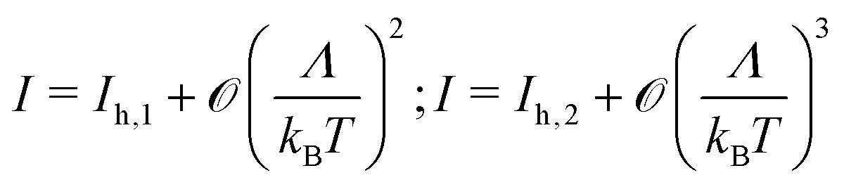
Analytical equations like Richardson–Dushman's or Shockley's provided a general, if simplified conceptual background, which was widely accepted in conventional electronics and made a fundamental contribution to advances in the field. In the attempt to develop a (highly desirable, but so far missing) counterpart for molecular electronics, in this work, we deduce a general analytical formula for the tunneling current through molecular junctions mediated by a single level that is valid for any bias voltage and temperature. Starting from this expression, which is exact and obviates cumbersome numerical integration, in the low and high temperature limits we also provide analytical formulas expressing the current in terms of elementary functions. They are accurate for broad model parameter ranges relevant for real molecular junctions. Within this theoretical framework we show that: (i) by varying the temperature, the tunneling current can vary by several orders of magnitude, thus debunking the myth that a strong temperature dependence of the current is evidence for a hopping mechanism, (ii) real molecular junctions can undergo a gradual (Sommerfeld–Arrhenius) transition from a weakly temperature dependent to a strongly (“exponential”) temperature dependent current that can be tuned by the applied bias, and (iii) important insight into large area molecular junctions with eutectic gallium indium alloy (EGaIn) top electrodes can be gained. E.g., merely based on transport data, we estimate that the current carrying molecules represent only a fraction of f ≈ 4 × 10⁻⁴ out of the total number of molecules in a large area Au–S–(CH2)13–CH3/EGaIn junction.
1 Introduction
Although representing only a small fraction compared to the overwhelming majority of studies conducted at room temperature, a number of investigations on charge transport in molecular junctions at variable temperature have been carried out in the past.1–35 Charge flow through molecular junctions can occur via a single-step tunneling mechanism or via a two-step hopping mechanism. Whether the measured current depends on temperature or not is taken by conventional wisdom as an expedient criterion to assign a specific case to hopping or tunneling, respectively. Presumably the reason why experimentalists resort(ed) to this pragmatic criterion can easily be understood. Most model theoretical approaches36–43 were developed for zero temperature (T = 0) and, if at all and even if deduced for T = 0, compact analytical formulas enabling straightforward I–V data fitting are rather scarce.39,43–45
A temperature dependence of the tunneling current (I) can arise due to the thermal broadening of the electronic Fermi distribution in electrodes. Recognizing this fact, several investigations drew attention that temperature dependent transport properties are compatible with a tunneling mechanism.1,8,23,26,32,46–53
Still, a fundamental question remains to be addressed: is the smearing of electrodes Fermi distribution sufficient to cause a temperature dependence strong enough to compete with that generated by hopping, which is known to yield currents exhibiting an exponential Arrhenius-type variation over several orders of magnitude? From a pragmatic standpoint, equally important is another question: is it possible to meet the experimentalists' legitimate need of having compact theoretical formulas expressing the tunneling current at arbitrary temperature obviating the cumbersome numerical integration (see eqn (4) below)?
In Section 2, an analytical exact formula will be presented which enables to express the tunneling current (I) mediated by a single level at any temperature and bias in terms of digamma functions of complex argument. Based on that formula, we will show that I can indeed vary over several orders of magnitudes (Section 4), making discrimination between tunneling and hopping a challenging matter (see Conclusion). We will also deduce analytical formulas for the current expressed in terms of elementary functions valid in the low and high temperature limits (Section 3); they turn out to be very accurate in very broad model parameter ranges (Section 5), complementary covering virtually all situations of interest for real molecular junctions.
As an application, starting from experimental current–voltage data measured for a real molecular junction,54 we will illustrate (Section 7) how a (Sommerfeld–Arrhenius52) transition from a current weakly varying with temperature at low T to a strongly temperature current at high T can be be controlled by tuning the applied bias voltage within a “tunneling-throughout” scenario.
As a by-product, we show how the presently considered single-level model of transport can provide important insight into large area molecular junctions with eutectic gallium indium alloy (EGaIn) top electrodes.
2 Model and exact formula for the current at arbitrary temperature
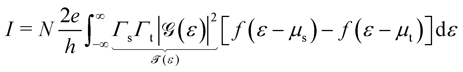
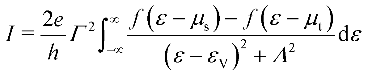
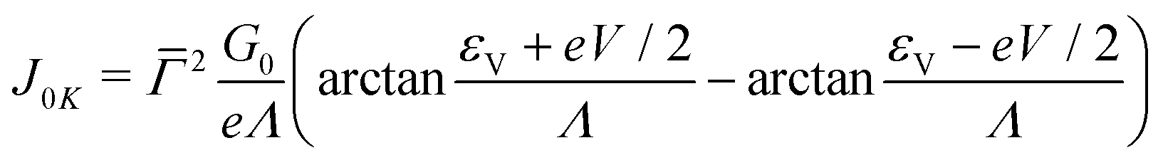
The Keldysh nonequilibrium formalism allows to express the tunneling current through a single molecule mediated by a single level (molecular orbital, MO) of energy εV by36,55| | 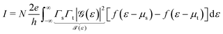 | (1) |
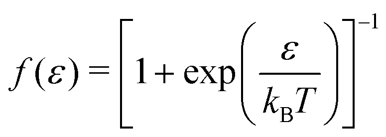
where 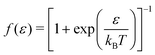 is the Fermi–Dirac distribution, and μs,t = ±eV/2 are the chemical potentials of the electrodes (“substrate s and “tip/top” t).
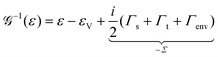
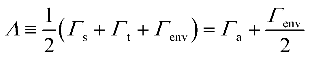
Key quantities in the above equation are the MO-electrode electronic couplings Γs,t, which also enter the retarded Green's function G of the embedded molecule via Dyson's equation
| |  | (2) |
We emphasize that although for the sake of convenience we will simply write
εV almost everywhere, various forward-backward asymmetries can yield a bias dependent MO energy offset,
e.g.and all the formula presented below hold for a general bias dependent quantity
ε0(
V) not even restricted to the (linear in
V) form mentioned above.
Notice that, along with electrodes' contribution Γs,t, we have also included in the Dyson eqn (2) an additional (“extrinsic”) contribution to the self-energy expressed via Γenv. This is requested by the physical reality. Except for genuine single-molecule setups—e.g., mechanically controlled break junctions (MC-BJ)—, the current carrying molecules are placed in an environment. In interaction with the surrounding—whether molecules of a solvent, neighboring molecules from a self-assembled monolayer, possibly also interaction in a cavity—the sharp delta-shape MO of an isolated molecule (gas phase) acquires a finite width quantified by Γenv. The Green function ![[capital G, script]](https://www.rsc.org/images/entities/char_e112.gif) of eqn (2) may refer to a molecule linked to one electrode (Γt ≡ 0)—the case in a ultraviolet photoelectron spectroscopy (UPS) “half-junction” setup—or linked to two electrodes—the case of molecular junctions, whatever the (coherent one-step tunneling or incoherent two-step sequential) transport mechanism; it does not matter, a nonvanishing Γenv can exist in all these cases.
of eqn (2) may refer to a molecule linked to one electrode (Γt ≡ 0)—the case in a ultraviolet photoelectron spectroscopy (UPS) “half-junction” setup—or linked to two electrodes—the case of molecular junctions, whatever the (coherent one-step tunneling or incoherent two-step sequential) transport mechanism; it does not matter, a nonvanishing Γenv can exist in all these cases.
Noteworthily, this reality needs not be accounted for phenomenologically. Whether referring to an UPS setup or to a molecular junction under bias the retarded Green's function (within an equilibrium formalism56 or in a nonequilibrium Keldysh formalism,36,55 respectively) can naturally account for this reality. In the Dyson eqn (2) underlying the present single level model, Γs,t and Γenv are accounted for on the same footing.
The assumption of a self-energy Σ independent of energy (ε)—which underlines the ubiquitous Lorentzian transmission ![[scr T, script letter T]](https://www.rsc.org/images/entities/char_e533.gif) (ε)—is legitimate in the case of metal electrodes possessing flat energy bands and environments without special features around the Fermi energy. In the same vein and for the sake of simplicity, we did not explicitly consider interactions of the envisaged molecule with electrodes and surrounding (see above) yielding a nonvanishing contribution to the real part of the self-energy Σ in eqn (2). All these effects amount to renormalize the value of ε0 entering eqn (3).
(ε)—is legitimate in the case of metal electrodes possessing flat energy bands and environments without special features around the Fermi energy. In the same vein and for the sake of simplicity, we did not explicitly consider interactions of the envisaged molecule with electrodes and surrounding (see above) yielding a nonvanishing contribution to the real part of the self-energy Σ in eqn (2). All these effects amount to renormalize the value of ε0 entering eqn (3).
| |  | (4) |
| | 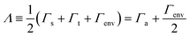 | (6) |
Notice that, after replacing
Γa by
Λ, all formulas presented in our earlier works (
e.g., ref.
43,
52,
53 and
57) in terms of the geometric (“effective”) and arithmetic average (
Γg and
Γa) remain valid although a possible contribution of the surrounding environment to the MO width (
Γenv) has not been explicitly mentioned. To avoid possible confusions (see ref.
58 and
57), we reiterate that the presently defined
Γ's may differ by a factor of two from quantities denoted by the same symbol by other authors.
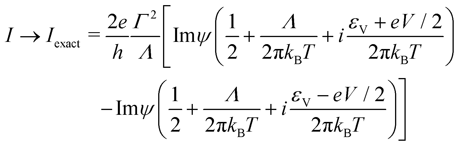
Expressed as product of a Lorentzian and a difference of Fermi function, the integrand entering eqn (4) is similar to that encountered in other phenomena (e.g., superconductivity59 or charge density waves60) for which contour integration is known to yield exact formulas expressed in terms of Euler's digamma function ψ of complex argument z (ψ(z) ≡ dΓ(z)/dz, Γ being here Euler's gamma function). Integration of eqn (4) can be carried out exactly and leads to the following form
| |  | (7) |
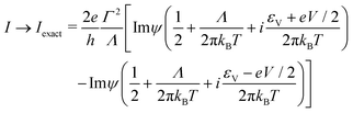
Noteworthily,
eqn (7) is exact at arbitrary temperature
T and bias
V within the single level model with Lorentzian transmission. Limitations of this model have been discussed recently
57,61 and will not be repeated here. The above formula generalizes various particular results deduced for
Γenv ≡ 0,
8,25,40,41,43,55,62–64 to which we will also refer below.
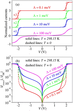
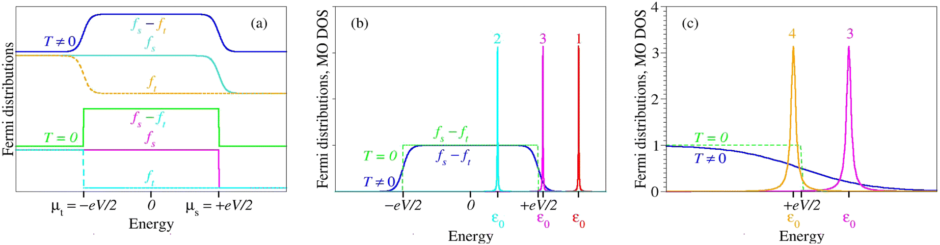
Putting in more physical terms, thermal fluctuations give rise to smeared Fermi distributions fs,t(ε) = f(ε − μs,t) in electrodes that appreciably differ from the zero temperature step (Heaviside) shape within ranges of width on the order of kBT around the electrochemical potentials μs,t = ±eV/2 (Fig. 1a). The temperature has a negligible impact on situations wherein the energy ε0 of dominant transport channel lies far away from resonance (curves 1 and 2 in Fig. 1b). However, the tunneling current can acquire a significant dependence on temperature in cases where a narrow enough transmission curve (i.e., sufficiently small Λ) appreciably overlaps with one of the two energy ranges affected by thermal smearing (curves 3 and 4 in Fig. 1b and c). More precisely, the temperature effect is stronger in situations slightly below resonance (εV ≲ μs, curve 4 in Fig. 1c) than slightly above resonance (εV ≳ μs, curve 3 in Fig. 1b and c). As illustrated in Fig. 1c, in the former case the current I(→Iexact) at temperature T can be substantially larger than the current at T = 0 denoted by I0K below (cf.eqn (8a)), while in the latter case I is at least half the value of I0K.
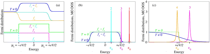 |
| | Fig. 1 (a) A nonvanishing temperature smears out the electrode Fermi distributions. (b) Negligible far away from resonance (curves 1 and 2), the effect of thermal broadening becomes important when the transmission peak comes into resonance with the electrochemical potential of one electrode (curve 3). (c) Thermal effects are more pronounced below resonance (curve 4) than above resonance (curve 3) because the overlap is larger in the former case. | |
3 Analytical expressions in the low and high temperature limits
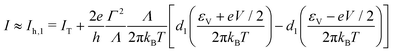
3.1 Current of low temperatures
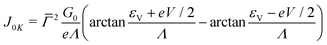
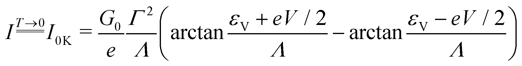
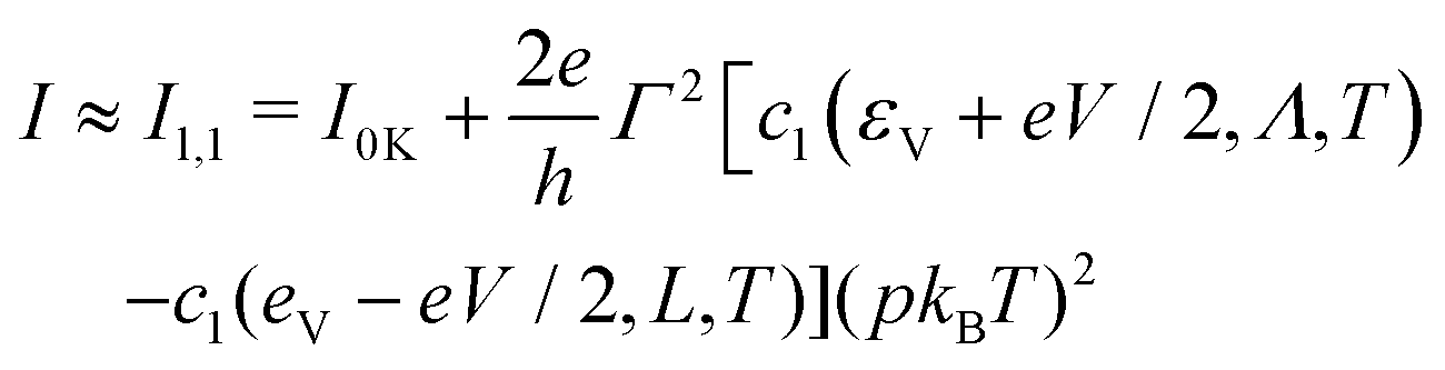
The zero temperature limit (I ≈ I0K) of eqn (7)| | 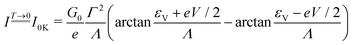 | (8a) |
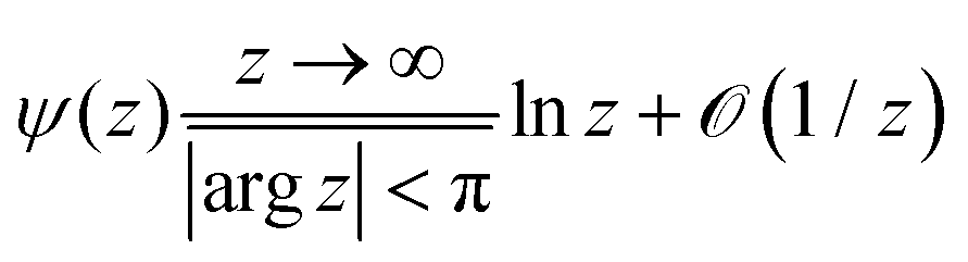
is recovered using the asymptotic expansion (eqn (6.3.18) in ref. 65)
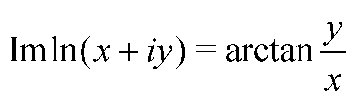
along with the identity
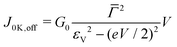
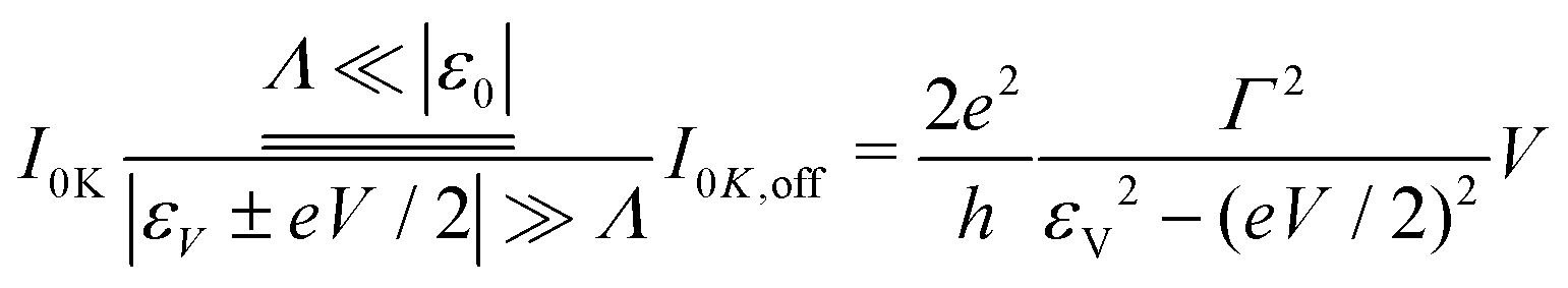
An important case of the low temperature limit is the off-resonant transport, for which eqn (8a) acquires a particularly appealing form43,57| | 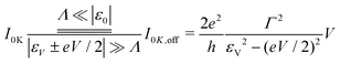 | (8b) |
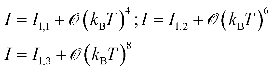
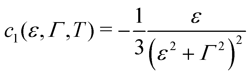
Low temperature (thermal) corrections to current can be deduced by expanding the digamma function in powers T65,66 or via Sommerfeld expansions67,68| |  | (9a) |
| | 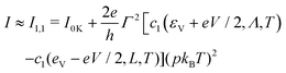 | (9b) |
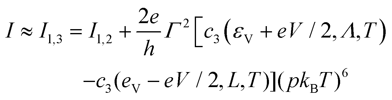
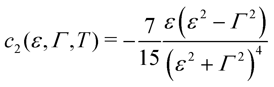
| | 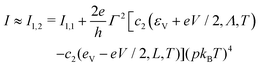 | (9c) |
| | 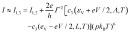 | (9d) |
where| |  | (9e) |
| | 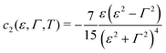 | (9f) |
| |  | (9g) |
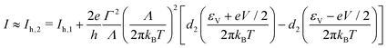
3.2 Current at high temperatures
The identity (cf. eqn (6.3.12) of ref. 65)
yields the formula for current valid in the high temperature limit 
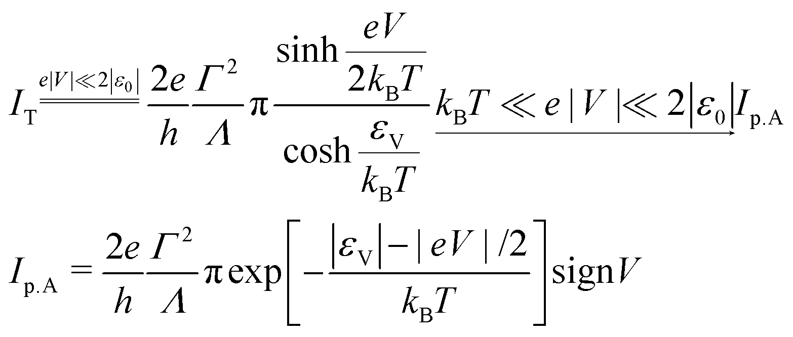
| |  | (10a) |
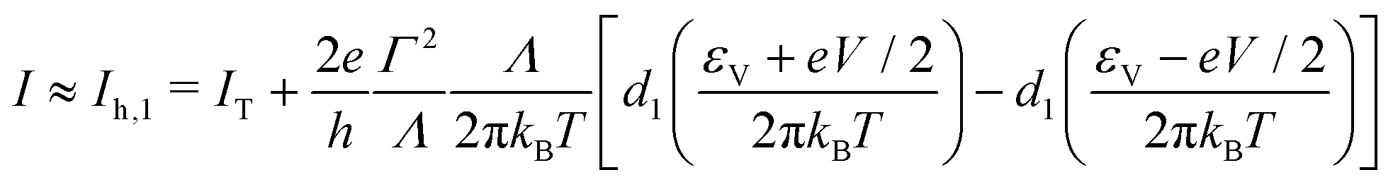
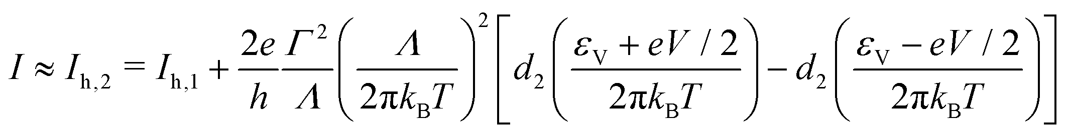
| |  | (10b) |
Above, the subscript p.A stands for “pseudo-Arrhenius” to emphasize that, in the limit specified, the tunneling current exhibits an Arrhenius-type dependence on temperature, which is routinely (or, better, “abusively”, see Introduction) considered characteristic for the hopping mechanism.
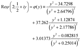
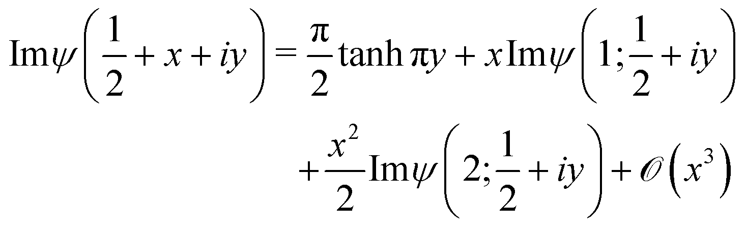
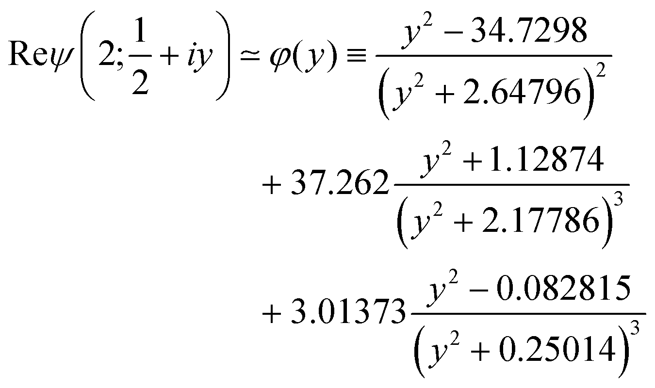
Series expansion in powers of x ≡ Λ/(2πkBT) in terms of polygamma functions ψ(n;z) ≡ dnψ(z)/dzn
| | 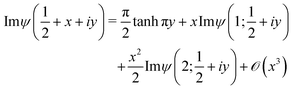 | (10c) |
allows to deduce corrections to
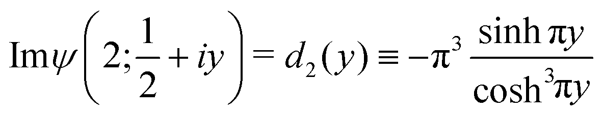
eqn (10a). Unlike the imaginary part of the tetragamma function (
ψ′′(
z) ≡
ψ(2;
z)), which can be expressed analytically in terms of elementary functions for
z = 1/2 +
iy| | 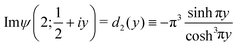 | (10d) |
the imaginary part of the trigamma function (
ψ′(
z) ≡
ψ(1;
z)) entering
eqn (10c) cannot. However, we found that it can be accurately interpolated numerically (see
Fig. 2a)
| | 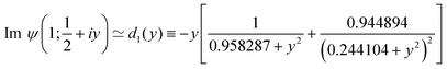 | (10e) |
We thus arrive at the following expressions applicable for MO broadening smaller that the thermal smearing of electrode Fermi functions (quantified by
Λ smaller than
kBT) characterizing transport data that exhibit a pronounced temperature dependence
| |  | (10f) |
| |  | (10g) |
| |  | (10h) |
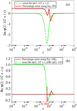 |
| | Fig. 2 The deviations of the numerical interpolation functions (a) d2(y) of eqn (10e) and (b) φ(x) of eqn (11k) from Im![[thin space (1/6-em)]](https://www.rsc.org/images/entities/char_2009.gif) ψ′(1/2 + iy) and Reψ(2; 1/2 + iy), respectively are smaller than half of percent. ψ′(1/2 + iy) and Reψ(2; 1/2 + iy), respectively are smaller than half of percent. | |
Notice that, similar to c1,2,3 (cf.eqn (9e)), the quantities d1,2 are expressed in terms of elementary functions (cf.eqn (10e) and (10d)). This is important for potential applications to processing transport data exhibiting substantial dependence temperature; special functions (digamma ψ in this specific case) of complex argument (cf.eqn (7)) are not implemented in software packages (like ORIGIN or MATLAB) routinely utilized by experimentalists for data fitting.
3.3 Analytical expressions for the zero bias conductance
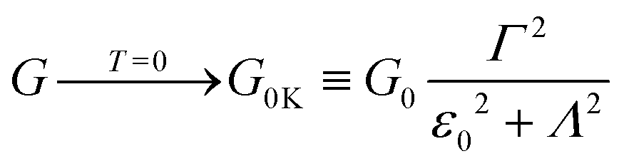
In the zero bias limit (V → 0), eqn (7) recovers the recently deduced formula for the exact ohmic conductance G.52 It is expressed in terms of the trigamma function (ψ′(z) = dψ(z)/dz)| | 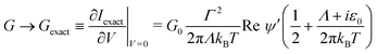 | (11a) |
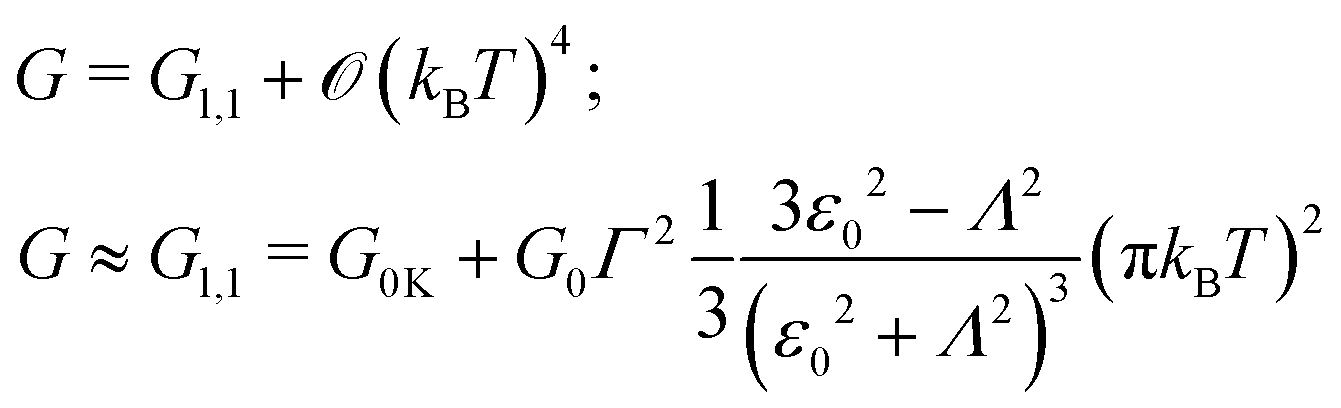
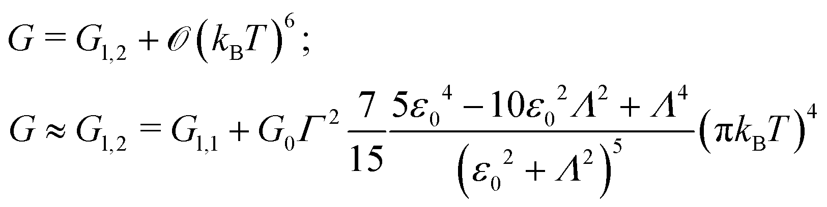
Thermal corrections to the zero temperature conductance G0K| | 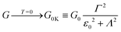 | (11b) |
obtained from the asymptotic expansion of the digamma function read| | G = G0K + ![[scr O, script letter O]](https://www.rsc.org/images/entities/char_e52e.gif) (kBT)2 (kBT)2 | (11c) |
| | 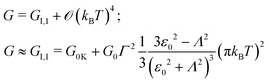 | (11d) |
| | 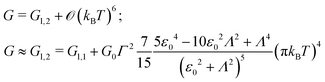 | (11e) |
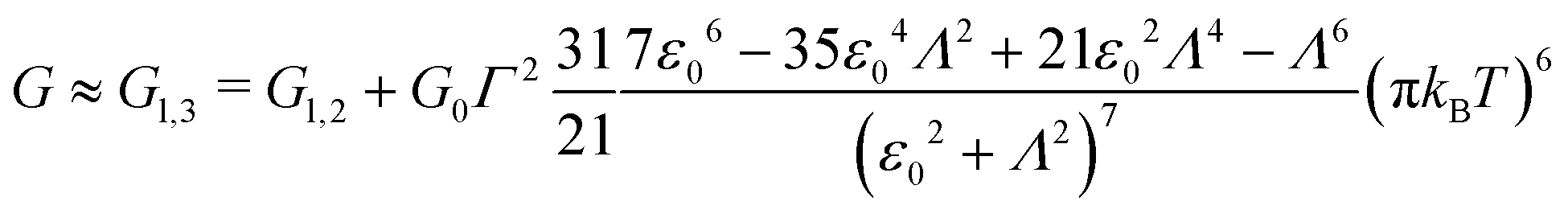
| | | G = Gl,3 + (kBT)8; | (11f) |
| | 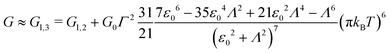 | (11g) |
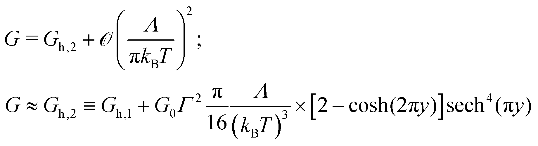
Analytical expressions in the high temperature limit (Λ smaller than πkBT) deduced previously52,53 are included for the reader's convenience (y ≡ ε0/(2πkBT))| | 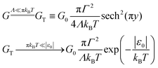 | (11h) |
| | 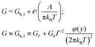 | (11i) |
| |  | (11j) |
| |  | (11k) |
The high accuracy of the numerical interpolation expressed by eqn (11k) is depicted in Fig. 2b.
4 Can the temperature impact on the transport by tunneling be as strong as on the transport by hopping?
To reiterate what we have mentioned in Section 2, all the above analytical formulas deduced for the tunneling current hold for MO energy offsets ε0(V) exhibiting an arbitrary dependence on the applied bias V, including in particular the case of nonvanishing Stark strengths γ ≠ 0. In this section, for simplicity, we confine ourselves to present numerical results for the bias independent case (ε0(V) = ε0, γ = 0). Because the charge conjugation invariance of this model yields equal currents computed for +ε0 and −ε0 and symmetric I–V curves (I(−V) = −I(V)), we can restrict ourselves to positive ε0 and V without loss of generality.
As said, traditionally a strongly temperature dependent transport was considered as a fingerprint for a hopping mechanism, but we showed above that the thermal broadening of electron Fermi distributions in electrodes makes the tunneling current dependent on temperature (see also Fig. 3). Can the tunneling current expressed by the above formulas vary over orders of magnitude if the temperature varies within experimentally relevant ranges, challenging thereby the hopping mechanism or the occurrence of a tunneling-hopping transition?
 |
| | Fig. 3 Currents at T = 298.15 K (solid lines) and T = 0 (dashed lines) normalized at the plateau value Λ/(πΓ2) for various values of Λ in (a) linear and (b) logarithmic y scale. For clarity, in panel a they are shifted vertically as indicated in the legend. | |
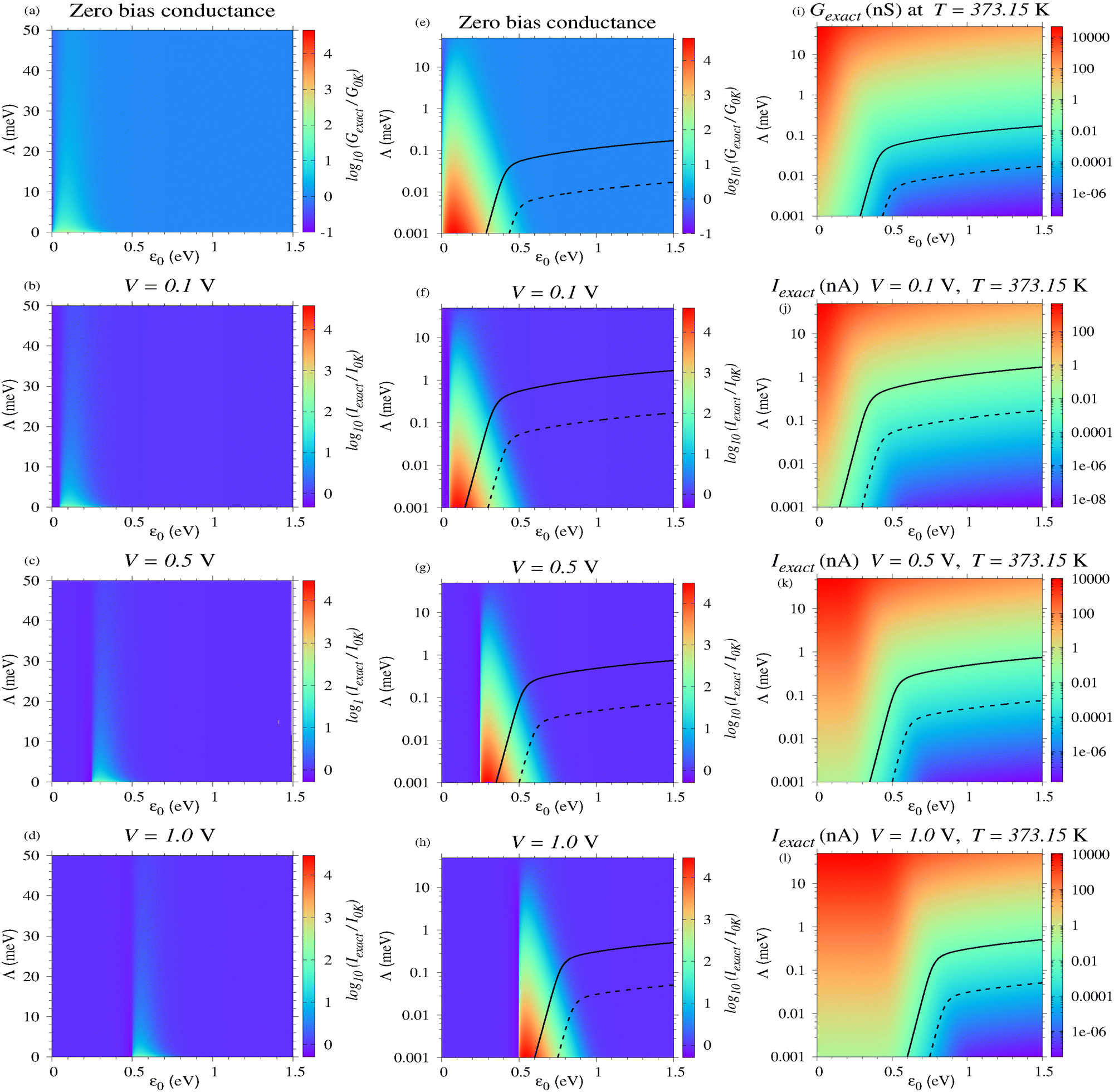
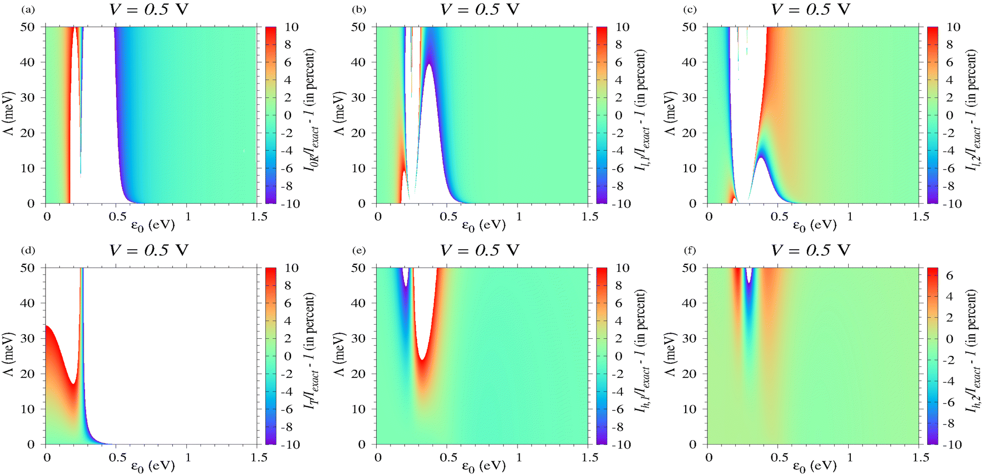
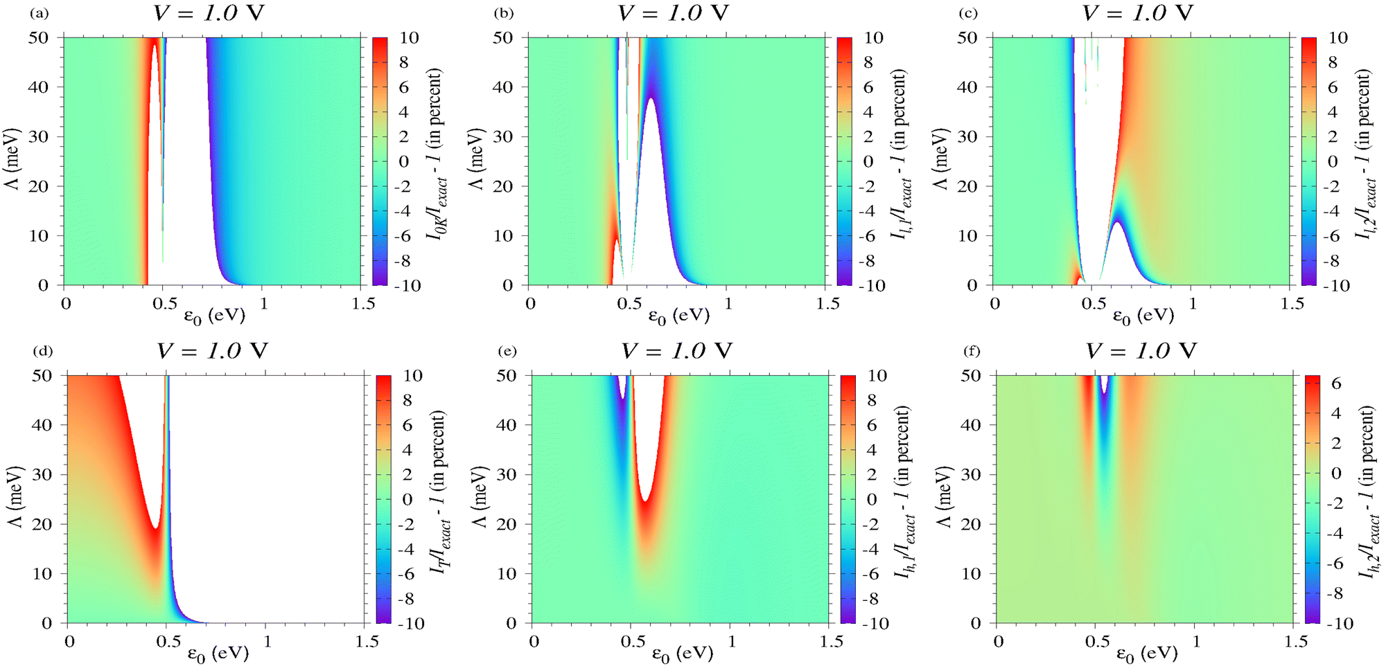
The numerical results collected in Fig. 4 offer the (positive) answer to this question. The first and second columns of Fig. 4 (panels a to d and e to h, respectively) depict the thermal excess quantified by the ratio of the exact conductance Gexact (eqn (11a)) and the exact current Iexact (eqn (7)) computed at T = 373.15 K (kBT = 32.2 meV) and several biases (V = 0.1; 0.5; 1.0 V) and their counterparts G0K and I0K at the same biases but at T = 0 (eqn (11b) and (8a), respectively) for the model parameter ranges 1 meV ≤ ε0 ≤ 1.5 eV and 0.001 meV ≤ Λ ≤ 50 meV. (We chose T = 373.15 K for illustration, as a reasonable value for the highest temperature of any practical interest.) Inspection of these panels indicates a current thermal enhancement up to three to four orders of magnitudes for a sufficiently small Λ and MO level outside the Fermi window but no very far away from resonance (say, e|V|/2 < |ε0| ≲ e|V|/2 + 10kBT).
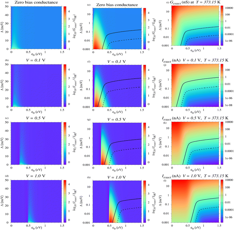 |
| | Fig. 4 (a)–(h) Ratio of the relevant transport properties (conductance Gexact and current Iexact) computed at T = 373.15 K and values of bias V indicated relative to their counterparts at T = 0 K (G0K and I0K, respectively). The model parameter Λ is depicted both in linear and (to better visualize the order of magnitude) logarithmic scale (panels a to d and e to h, respectively). By and large, the main effect of the bias V is a horizontal energy shift eV/2 of the parameter ranges corresponding to substantial thermal enhancement, which becomes more pronounced as the resonance (ε0 = eV/2) is approached from below (ε0 ≳ eV/2). Diagrams for the zero bias conductance in nS (i) and (j)–(l) current in nA at T = 373.15 K. The parameter regions wherein Gexact > 1 pS (panel i) and Iexact > 10 pA (panels j–l), which can be considered reasonable lower bound values for experimental accessibility, lie below the solid and dashed lines. See the main text for details. | |
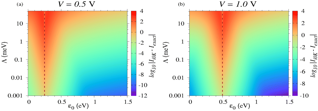
To avoid misunderstandings related to the appearance of Fig. 4, we emphasize that, unlike the current thermal excess Iexact/I0K, which is highly asymmetric around resonance—very large below resonance (Iexact/I0K ≫ 1 for e|V|/2 ≲ |ε0|) but not too small above resonance (1 > Iexact/I0K > 1/2 for e|V|/2 ≳ |ε0|)—the absolute difference |Iexact − I0K| is practically symmetric around resonance (e|V|/2 = |ε0|); compare Fig. 4 with Fig. 5. Along with the strong thermal enhancement, convincing oneself that the conductance/current are reasonable large to be measurable in the pertaining model parameter ranges is an equally important aspect that deserves consideration. Therefore, Fig. 4 also indicates the parameter ranges wherein the values G and I are larger than 1 pS and 0.01 pS, and 10 pA and 0.1 pA, respectively. These values correspond to the regions above the continuous and dashed lines depicted in panels e to l. (We do not show these lines in panels a to d because the linear y-scale would make visibility problematic.) Above, the larger values 1 pS and 10 pA were chosen as realistic lowest values still measurable for single molecule junctions. The values one hundred times lower (0.01 pS and 0.1 pA) can be taken as the counterpart for CP-AFM junctions, which consist of ∼100 molecules per junction.69
 |
| | Fig. 5 Unlike the relative deviations depicted in Fig. 4, the absolute deviations of I0K from Iexact are nearly symmetric around resonance |ε0| = e|V|/2. This is illustrated here for two bias values: (a) V = 0.5 V and (b) V = 1.0 V. | |
To sum up, we conclude that the impact of temperature on the transport via a single step tunneling mechanism can definitely be as strong as that the impact on the two-step hopping mechanism, which was traditionally associated to a pronounced temperature dependence.
5 How accurate are the analytical approximations expressed in terms of elementary functions?
To illustrate the accuracy of the approximate formulas for conductance and current deduced in Section 3.3, we present comparison with the exact eqn (11a) and (7) at T = 373.15 K at several biases: V = 0; 0.1; 0.5; 1.0 V (Fig. 6–9, respectively).
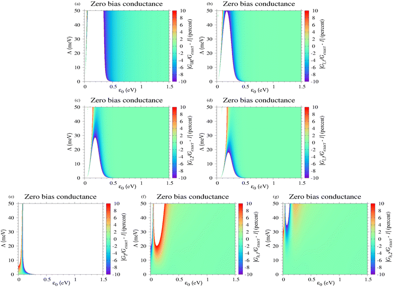 |
| | Fig. 6 Percentage deviations of the zero bias conductance computed by the various methods indicated in each of the panels a to g with respect to the value computed exactly at T = 373.15 K. | |
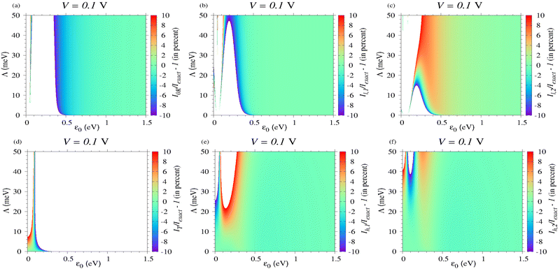 |
| | Fig. 7 Percentage deviations of the current computed at V = 0.1 V and T = 373.15 K by the various methods indicated in each of the panels a to f with respect to the value computed exactly. | |
 |
| | Fig. 8 Percentage deviations of the current computed at V = 0.5 V and T = 373.15 K by the various methods indicated in each of the panels a to f with respect to the value computed exactly. | |
 |
| | Fig. 9 Percentage deviations of the current computed at V = 1.0 V and T = 373.15 K by the various methods indicated in each of the panels a to f with respect to the value computed exactly. | |
Methodologically, performing (Sommerfeld) expansions in powers of T (more precisely, in even powers of T because odd powers do not contribute) is the most straightforward way to account for thermal effects on the tunneling current.67,68 Doing so, eqn (9b)–(9d) and (11d)–(11f) can be recovered after some tedious calculations. Inspection reveals that, including the first order correction (∝T2), Gl1, and Il,1 represent a better description with respect to the zero temperature quantities G0K and I0K; compare Fig. 6b, 7b, 8b and 9b with Fig. 6a, 7a, 8a and 9a, respectively. Still, although the second order correction (∝T4) depicted in Fig. 6c, 7c, 8c and 9c represents a further improvement, expansion in powers of kBT/Λ inherently fails for sufficiently small Λ, when the transport strongly depends on temperature.
Unfortunately, although appealing simple, the expressions for GT and IT deduced in the high temperature limit (eqn (11h) and (10a)) appear to have a very restricted validity; see Fig. 6d, 7d, 8d and 9d. Below resonance, IT is only reasonably in a very narrow parameter range. And yet, the formulas deduced by adding first and second high temperature corrections (Gh,1, Gh,2, eqn (11i) and (11j)) and Ih,1, Ih,2, (eqn (10g) and (10h)) turn out to be very accurate even in the parameter ranges where the thermal impact is very pronounced; see Fig. 6e, f, 7e, f, 8e, f, and 9d, f.
Although the main aim of the present paper is to present general analytical formulas for the current through molecular junctions mediated by a single (dominant) channel rather than discussing applications to real junctions, in the next two sections we will analyze I–V curves measured for junctions fabricated using two extreme platforms: a large area junction with top electrode of eutectic gallium indium alloy (EGaIn)70 (Section 6) and a single-molecule junction54 (Section 7).
6 Analyzing transport data of a specific large area EGaIn-based molecular junction
In the above presentation, emphasis was on the temperature dependence of the tunneling current. However, we also want to draw attention on an effect that did not explicitly entered the foregoing discussion: the possibility that the MO of the active molecule acquires a significant width from the surrounding medium (Γenv ≠ 0). Furthermore, by focusing on a specific large area EGaIn junction below, we also aim at illustrating that/how the single level model can help to determine the fraction f of the current carrying molecules Neff, which represent only tiny amount of the total (nominal) number of molecules Nn in junction (f ≡ Neff/Nn ≪ 1).21,71–74 To better underline the importance of the aforementioned, we have intentionally chosen experimental results reported for a real junction wherein the impact of temperature is negligible (cf.Fig. 10c): a large area EGaIn-based junction fabricated with 1-tetradecanethiol SAMs (C14T) chemisorbed on gold electrode Au–S–(CH2)13–CH3/EGaIn.70 Typically, experiments on large area molecular junctions report values for the current density J = J(V) (in A cm−2) rather than I = I(V) (in A). For this reason, we recast eqn (7), (8a) and (8b) needed below in terms of current densities| | 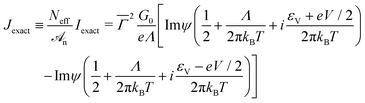 | (12a) |
| |  | (12b) |
| |  | (12c) |
Here| | 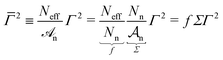 | (13) |
and Σ is the SAM coverage. Recall that εV entering eqn (6) is a shorthand for ε0(V), cf.eqn (3).
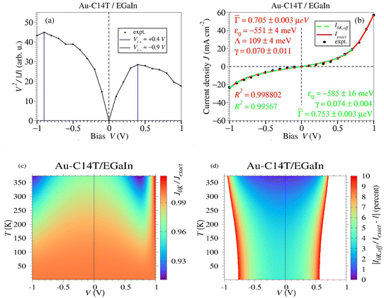 |
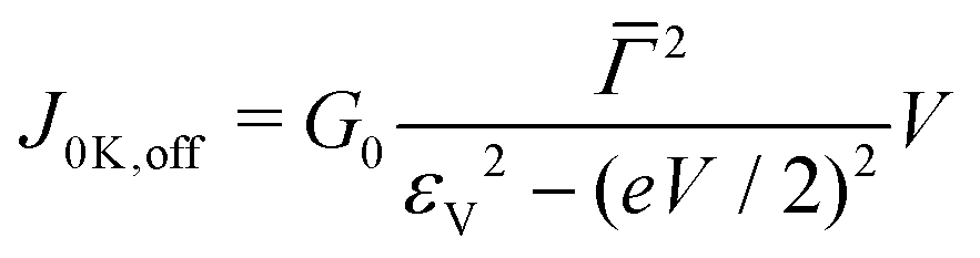
| | Fig. 10 (a) Plots of V2/|I| versus V enabling the determination of the values of the transition voltages Vt± needed to properly define the bias range where eqn (12b) applies. (b) Correctly utilized, eqn (12b) is able to reproduce (green curve) the experimental data (black points) for the large area Au-C14T/EGaIn junction of ref. 70 with an accuracy comparable to that of the exact eqn (12a) (red curve). Diagrams revealing (c) that thermal effects are negligible in the Au-C14T/EgaIn junction envisaged and (d) that, when applied for the bias range for it was devised,43eqn (12b) is able to describe quantitatively I–V data in large area junctions. See the main text for details. | |
Reliable values of the parameters ε0![[capital Gamma, Greek, macron]](https://www.rsc.org/images/entities/i_char_e0ba.gif) , and γ can be obtained by fitting the experimental I–V data with any of eqn (6), the pertaining results are presented in Table 1 and Fig. 10. Noteworthily, as reiterated again and again,47,57,58 to correctly employ our model proposed in ref. 43, eqn (12c) should be applied to bias ranges |V| ≲ 1.2Vt (cf.Fig. 10d). Here, the transition voltage Vt is defined as the bias where V2/|I| is maximum (Fig. 10a). All three fitting curves successfully reproduce the measurements (cf.Fig. 10b). The good agreement between these methods demonstrates that in the large area Au-C14T/EaGaIn considered thermal effects are negligible (j0K ≈ jexact, cf.Fig. 10c), and that the transport in off-resonant situations can be reliably described by j0K,off (≈ jexact, see green curve in Fig. 10b).
, and γ can be obtained by fitting the experimental I–V data with any of eqn (6), the pertaining results are presented in Table 1 and Fig. 10. Noteworthily, as reiterated again and again,47,57,58 to correctly employ our model proposed in ref. 43, eqn (12c) should be applied to bias ranges |V| ≲ 1.2Vt (cf.Fig. 10d). Here, the transition voltage Vt is defined as the bias where V2/|I| is maximum (Fig. 10a). All three fitting curves successfully reproduce the measurements (cf.Fig. 10b). The good agreement between these methods demonstrates that in the large area Au-C14T/EaGaIn considered thermal effects are negligible (j0K ≈ jexact, cf.Fig. 10c), and that the transport in off-resonant situations can be reliably described by j0K,off (≈ jexact, see green curve in Fig. 10b).
Table 1 Model parameter values obtained by fitting the experimental J–V data70 to the formulas for the current indicated in the first column
| Method |
ε
0 (eV) |
Λ (meV) |
(μeV nm−1) |
γ
|
f
|
Γ
env
|
Γ
env/(2Λ) (%) |
R
2
|
|
J
exact
|
−0.551 ± 0.004 |
109 ± 0.004 |
0.705 ± 0.003 |
0.07 ± 0.01 |
4.3 × 10⁻⁴ |
217.3 |
99.7 |
0.998802 |
|
J
0K
|
−0.535 ± 0.004 |
115 ± 0.004 |
0.695 ± 0.002 |
0.07 ± 0.01 |
4.2 × 10⁻⁴ |
229.3 |
99.7 |
0.99884 |
|
J
0K,off
|
−0.585 ± 0.004 |
— |
0.753 ± 0.003 |
0.074 ± 0.004 |
4.9 × 10⁻⁴ |
— |
— |
0.99567 |
6.1 Working equations for large area EGaIn junctions
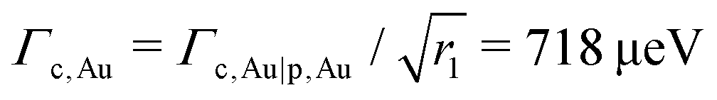
Let us first recast eqn (5), (6) and (13) in a form more specific for junctions whose molecules are chemisorbed on a gold substrate (label c,Au) and physisorbed on EGaIn top electrode (label p,EGaIn) or CP-AFM gold tip (label p,Au)| |  | (14a) |
| |  | (14b) |
(from ref. 53)| | 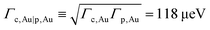 | (14c) |
(via ref. 75)
| |  | (14d) |
Above,
Γc,Au|p,EGaIn and
Γc,Au|p,Au are effective couplings (
cf. Section 2) of junctions chemisorbed on gold substrate and physisorbed on EGaIn and gold top electrodes, respectively.
Γ's with subscripts without vertical bar stand for individual HOMO-electrode couplings (recall that alkanethiols CnT exhibit p-pype HOMO-mediated conduction
75);
e.g,
Γp,X means p(hysical) coupling to electrode X(= Au,EGaIn). Let us now explain how we arrived at the numerical values entering
eqn (14b) and (14c).
The coupling ratios r1,2 of eqn (14b) were estimated recently.53 The value of r1 ≈ 1/37 was deduced by comparing the couplings of alkane thiols and alkane dithiols. The value of r2 ≈ 1/7 relies on the dependence of the coupling on the electrode work function.
To get Γc,Au|p,Au = 118 μeV in eqn (14c), we extrapolated the values of the effective coupling Γ(n)c,Au|p,Au → Γn ∝ exp(−βn/2) for CP-AFM alkanethiols CnT (H–S–(CH2)n−1–CH3) junctions (Au–CnT/Au). That is, we used the values of Γn (for n = 7, 8, 9, 10, 12) from Table 1 of ref. 75. The exponential scaling of Γnversus n follows from the exponential falloff Gn ∝ exp(−βn) of the low bias conductance Gn ∝ Γn2/(εn0)2, given the fact that the HOMO offset ε(n)0 of the CnT series is independent of size (n).75
6.2 Estimating the fraction of current carrying molecules and the extrinsic HOMO relaxation
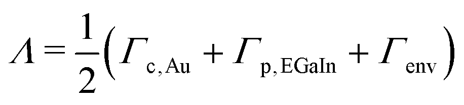
We will now explain how to use the values of and Λ obtained from I–V data fitting and the above working equations to estimate the fraction of the current carrying molecules f and the extrinsic contribution to the (HO)MO broadening Γenv.
6.2.1 Fraction of current carrying molecules f.
From the definition of r1 of eqn (14b), we use eqn (14c) to compute 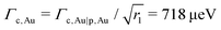 . Using again the definition of r1, we deduce
 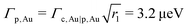 . From the definition of r2 of eqn (14b) we get Γp,EGaIn = r2Γp,Au = 0.456 μeV. From eqn (14a) we can now compute
  . With the value Σ = 3.5 mol nm−2 measured for the molecular coverage of alkanethiol SAMs,76 and the fitting parameter value = 0.705 μeV (Table 1), we can finally estimate viaeqn (14a) the fraction of the current carrying molecules
| fAu-C14T/EGaIn ≈ 4.3 × 10⁻⁴ |
This value is on the same order of magnitudes of other values of f reported for large area EGaIn-based junctions using methos completely different from the present one.20,53,77 Definitely, out of the total/geometric/nominal area at the EGaIn contact ![[scr A, script letter A]](https://www.rsc.org/images/entities/char_e520.gif) n, the area of the physical/electric/effective contact eff = fn is but a tiny fraction (f ≪ 1).
n, the area of the physical/electric/effective contact eff = fn is but a tiny fraction (f ≪ 1).
6.2.2 Extrinsic contribution Γenv to the (HO)MO width.
With the values for Λ (Table 1), Γc,Au, and Γp,EGaIn in hand, we use eqn (14d) and obtain Γenv ≈ 217.3 meV. This is a very important result. It demonstrates that the extrinsic contribution represents (Γenv/2)/Λ ≈ 99.7% of the total HOMO width. Compared to the contribution of the surrounding, the contribution of the electrodes the the HOMO broadening is completely negligible. To obtain the aforementioned values of f and Γenv we used the values of and λ obtained by fitting the experimental I–V data70 to the exact eqn (12a). The values collected in Table 1 reveal that these values do not significantly differ from the estimates for f and Γenv based on eqn (12b).
To end, it is worth emphasizing that the off-resonant single level model (eqn (12c)43) is also useful for large area EGaIn junctions. Eqn (12c) does not only reproduce I–V curves in nonlinear regime (green line in Fig. 10b) but also allows to reasonably estimate the fraction of current carrying molecules. The rather minor difference between the value f = 4.9 × 10⁻⁴ based on eqn (12c) and the “exact” value f = 4.3 × 10⁻⁴ deduced viaeqn (12a) is due to the fact, albeit smaller than |ε0|, Λ is not smaller that |ε0|/10, which is the condition for eqn (12c) to be very accurate.57,58
7 Predicting a bias-tuned Sommerfeld–Arrhenius transition in a real molecular tunnel junction
Let us now switch to a mechanically controlled break junction (MC-BJ) of 4,4′-biscyanotolane (BCT) with gold electrodes.54 Results for this junction are collected in Fig. 11. Fitting the digitized I–V data measured at room temperature (Fig. 1 of ref. 54) to eqn (7) at T = 298.15 K yielded an excellent fitting curves (R2 = 0.994, cf.Fig. 11a).
 |
| | Fig. 11 (a) The experimental I–V curve for a 4,4′-biscyanotolane (BCT) mechanically controlled break junction (MC-BJ) obtained by digitizing Fig. 1 of ref. 54 is excellently fitted by the theoretical current Iexact given by eqn (7) at T = 298.15 K. Curves computed using various approximate formulas for current with the optimized model parameters (see legend) are also presented. (b) Percentage deviations from the exact current of the current computed using the methods indicated in the legend shown in a bias range broader than the the bias range explored in experiment (depicted by vertical dashed lines). The thermal excess current Iexact/I0K depicted (c) as a function of temperature (T) at several bias values (V) and (d) in the (V, T)-plane. Notice the large values of Iexact/I0K in situations slightly below resonance. (e) At biases slightly below resonance (V = 0.95 V, eV ≲ 2|ε0|) Iexact switches from a weakly T-dependent (Sommerfeld) regime to a strongly T-dependent (Arrhenius-like) regime wherein it can be approximate by the expressions deduced for the low and high T limits, respectively. (f) Regions in the (V, T)-plane where eqn (8b) is accurate within the experimental accuracy. | |
Within the bias range sampled in experiment (|V| < 0.7 V),54 thermal effects are non-negligible (thermal excess higher than 10%) only at the ends of the experimental range: |V| > V10% = 0.607 V (eV10% ≈ 2(|ε0| − 3πkBT) ≈ 2(|ε0| − 10kBT)); see Fig. 11b. Except for biases very close to the highest experimental bias (V = 0.7 V), even the zero temperature expressions (I0K and I0K,off) are accurate; see Fig. 11e and f. For such situations, the low temperature expansion (Il,1, Il,2, and Il,3) provides an improved description over the zero temperature description (I0K and I0K,off, see Fig. 11b). More significant is however the high accuracy of the high-temperature approximations: at the small value Λ = 1.71 ± 0.01 meV ≪ kBT = 25.7 meV obtained by data fitting, even the lowest order expansion (Ih,1) excellently reproduces the exact current Iexact; higher order corrections embodied in Ih,2 are superfluous.
Beyond the bias range explored in ref. 54, the thermal current enhancement Iexact/I0K becomes more and more pronounced as the resonance value is approached from below (eV ≲ 2|ε0|) and the temperature is increased. Results up to the highest temperature of potential practical interest (T = 373.15 K) are presented in Fig. 11c–e. They show that for biases sufficiently close to resonance, values up to Iexact/I0K ≈ 20 can be reached. In such situations, a gradual Arrhenius–Sommerfeld transition52 can become observable (Fig. 11d).
In Table 2, we collect the model parameters ε0 (<0, HOMO conduction), Λ (= Γ, single-molecule junction fabricated with a symmetric molecular species) estimated from data fitting to the various formulas for the current. As visible there, applying the zero temperature formulas (I0K and I0K,off) to situations not enough far away from resonance and Λ ≪ kBT yielded an error of 22% in the value estimated for the HOMO offset and 15% for Γ.
Table 2 Model parameter values obtained by fitting the experimental BCT data54 to the various formulas for the current, as indicated in the first column
| Method |
ε
0 (eV) |
Γ = Λ |
γ
|
R
2
|
|
I
exact
|
−0.545 ± 0.002 |
1.71 ± 0.01 |
−0.0021 ± 0.0009 |
0.993551 |
|
I
h,1
|
−0.547 ± 0.002 |
1.73 ± 0.01 |
−0.0021 ± 0.0009 |
0.993513 |
|
I
h,2
|
−0.547 ± 0.002 |
1.72 ± 0.01 |
−0.0021 ± 0.0009 |
0.993513 |
|
I
0K
|
−0.472 ± 0.004 |
1.46 ± 0.02 |
−0.003 ± 0.001 |
0.992632 |
|
I
0K,off
|
−0.472 ± 0.004 |
1.46 ± 0.02 |
−0.003 ± 0.001 |
0.992632 |
|
I
l,1
|
−0.492 ± 0.004 |
1.50 ± 0.02 |
−0.003 ± 0.001 |
0.992729 |
|
I
l,2
|
−0.511 ± 0.003 |
1.55 ± 0.02 |
−0.003 ± 0.001 |
0.992809 |
|
I
l,3
|
−0.526 ± 0.003 |
1.58 ± 0.02 |
−0.003 ± 0.001 |
0.992860 |
8 Remarks on the applicability of presently deduced formulas
Going through the plethora of equations presented above, an experimentalist less interested in how they were mathematically deduced may ask what is the appropriate formula needed and how to proceed in transport data processing for a specific junction, fabricated with a specific molecule, specific electrodes, and a specific platform. This section and the next two sections aim at addressing such legitimate questions. Basically, within the model parameter ranges indicated, the formulas of Sections 2, 3 and 5 are general:
8.1 With regard to electrodes
They apply to all electrodes having flat conduction bands around the Fermi energy EFi.e., having a density of states practically independent of energy ρ(ε) ≈ ρ(EF). This translates into energy independent MO-electrode couplings (Γs,t(ε) ≈ Γs,t(EF) ∝ ρ(EF)τs,t2, see below). While this is not the case of semiconductors or graphene, it is definitely the case of all typical metals (like Ag, Au, Pt).78
8.2 With regard to molecules
The formulas apply to all molecules wherein the charge transport is dominated by a single level (MO), which is in most cases either the HOMO or the LUMO. The applicability of the single level description is often justified intuitively by the sufficiently large energy separation from the adjacent MOs. In fact, MOs' energetic separation may be a sufficient condition but is not a necessary condition. If, in some cases, a few highest occupied (e.g., HOMO and HOMO−1) or a few lowest unoccupied (e.g., LUMO and LUMO+1) have energies close to each other, they typically have different symmetries and/or different spatial (de)localization. The result is that, out of each group (of occupied or unoccupied MOs), only one MO has significantly overlap with the electronic states in metals. Due to different symmetry (and/or (de)localization) it can happen, e.g., that the (more distant from EF) HOMO−1 rather than the (closer to EF) HOMO has a larger hybridization with the single-electron states in the substrate (or tip/top) electrode. A larger hybridization means a transfer integral τs quantifying the charge transfer between HOMO−1 and substrate larger than that of the charge transfer between HOMO and substrate. This translates into MO–substrate (or tip) coupling Γs,t ∝ ρ(EF)τs,t2 dominated by the HOMO-1 and not by the HOMO.
8.3 With regard to the fabrication platform
With appropriate model parameter values (to be adequately estimated from data fitting), these formulas can be applied for molecular junctions fabricated using any platform, let it be MC-BJ, STM-BJ, CP-AFM or (as we have just seen in Section 6) EGaIn. It may be helpful to recall53 here that, like the model proposed in ref. 43, the present single level model does not assume negligible intermolecular interactions. An electron that tunnels across a molecule can interact with the adjacent molecules. Provided that electron exchange (transfer) between adjacent molecules is absent, the single level model “allows” intermolecular interactions to give rise to an extra MO shift (thence possible different values of ε0 for single-molecule, CP-AFM, and EGaIn junctions, a fact which will reflect itself in the best fitting estimates) and an extra level broadening expressed by Γenv.53 This is the rationale of “simply” multiplying the present expressions for current through a single molecule by the number of molecules per junction, as done earlier in case of CP-AFM junctions75,79,80 or in arriving at eqn (12) above.
9 Protocol for studying a specific junction
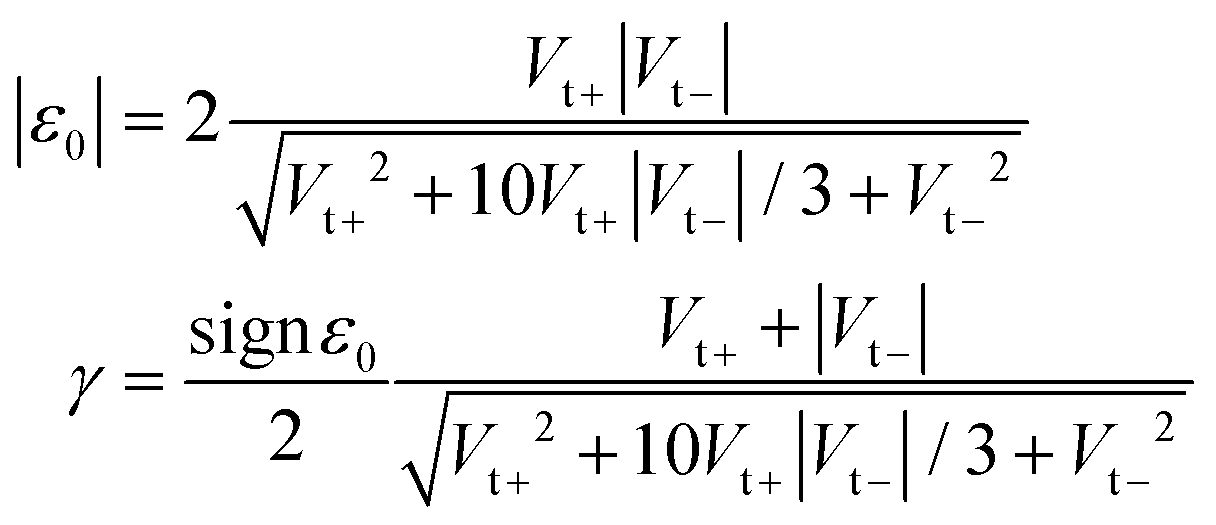
In view of the results presented above, assuming that room temperature I–V measurements for a specific molecular junction are available (which is the common case), we recommend the following steps for data processing: (i) start by plotting the measured data in coordinates (V2/|I|,V) and determine the transition voltages Vt± from the peak location (cf.Fig. 10a). Use our eqn (6) and (7) of ref. 43 (reproduced below for the reader's convenience) to estimate the magnitude of the MO offset |ε0| and γ
The MO offset ε0 is negative for p-type (normally, HOMO) conduction and positive for n-type (normally, LUMO) conduction. Recall that, whatever the formulas for the current utilized, the sign of ε0 cannot be merely determined from I–V curves measured for a given junction (= given molecule, given electrodes). Thermopower experiments to determine the sign of the Seebeck coefficient S or investigating junctions fabricated with a given molecule and electrodes having different work functions Φ.75,79,80 may settle this issue; positive (negative) S means negative (positive) ε0,81 higher (lower) current for larger Φ means negative75,79,80 (positive32) ε0.
Determine next the value of  using the low bias conductance G obtained from the slope of the measured I–V curve at low bias. With the values of ε0, Γ and γ thus obtained compare the measured curve with the simulated curve computed using our eqn (8b) in the bias range −1.2|Vt−| ≲ V ≲ 1.2Vt+. Alternatively, always in the bias range indicated (for which eqn (8b) applies), one can fit the measured data to I0K-off of eqn (8b) wherein ε0, Γ and γ are adjustable parameters. (ii) If attempt (i) fails to produce a good theoretical curve, fit data to I0K of eqn (8a) in the entire bias accessed experimentally with ε0, Γ, γ, and Λ as adjustable parameters. If the corresponding point (ε0K0, Λ0K) falls in the colored regions of Fig. 6a, 7a, 8a or 9a, this is evidence that the best fit values ε0K0, Γ0K, γ0K and Λ0K are reliable and that, at the corresponding bias, eqn (8a) is reliable. In other words, at the envisaged bias, thermal corrections to the current are negligible. Notice that (like eqn (8b) and (8a)) can hold up to a certain bias (e.g., V = 0.5 V) but can become inadequate at higher biases (e.g., V = 1 V) (see the example of Section 7). (iii) The failure of attempt (ii) indicates that (possibly only beyond certain biases) the temperature dependence of the current is significant. Generally speaking, whenever possible (e.g., using MATHEMATICA) fitting data to the exact eqn (7) is then most advisable. Otherwise the various analytical formulas for the current Il,1, Il,2, Il,2 of eqn (9) or Ih,1, Ih,2 of eqn (10) can be easier applied. Because they merely contain elementary functions the approximate formulas for Il,1, Il,2, Il,2, Ih,1, and Ih,2 are implementable in any fitting software package. Loosely speaking, the deeper the point (ε0K0, Λ0K) into the white (non-colored) regions mentioned under (ii) above, the stronger is the impact of T on the current at the corresponding bias. (iiia) For cases wherein the point (ε0K0, Λ0K) lies near the edge between colored and non-colored regions of Fig. 6a, 7a, 8a, or 9a, thermal effects are rather weak, and using the formula of Il,1 of eqn (10g) for data fitting is advisable. If the best fitting point (εl,10, Λl,1) obtained fitting the experimental I–V curve to eqn (10h) is found in the colored regions of Fig. 6b, 7b, 8b, or 9bIl,1 provides an accurate description and the fitting parameters εl,10, Γl,1, γl,1, and Λl,1 are good estimates of the corresponding quantities. Otherwise, performing and inspecting the results of data fitting based on Il,2 of eqn (9c) (and then Il,3 of eqn (9d) if the case) follows in the next step. (iiib) If the point (ε0K0, Λ0K) lies deep inside the white (non-colored) regions of Fig. 6a, 7a, 8a, or 9a, thermal effects are strong, and the formula deduced via high temperature expansions (Ih,1 of eqn (10g)) and Ih,2 of eqn (10h) should be employed for reliably estimate the parameters ε0, Γ, γ, and Λ for the junction under investigation. In cases where (iiib) applies, performing I–V measurements at variable temperature is highly desirable, and the issues related to the Sommerfeld–Arrhenius transition addressed in the next section deserve consideration.
10 Tunneling-throughout Sommerfeld–Arrhenius scenario versus tunneling-hopping transition: a too challenging a dilemma?
For a Sommerfeld–Arrhenius transition to occur in a specific molecular junction, the parameters ε0 and Λ at given bias V should fall in regions in the plane (ε0, Λ) where the current thermal enhancement Iexact/I0K is sufficiently large (say, at least Iexact/I0K ≳ 10), like the red curve in (Fig. 11e). The color coding of Fig. 6a, 7a, 8a, or 9a precisely depicts which combination of values (ε0,Λ,V) is “eligible” for a Sommerfeld–Arrhenius transition (i.e., Iexact/I0K is reasonably large). Experimental curves for current versus inverse temperature having a shape resembling the red curve in Fig. 11e have been measured in the past for several molecular junctions. Examples include junctions fabricated with: conjugated oligo-tetrathiafulvalenepyromelliticdiimideimine (OPTIn; OPTI2 in Fig. 6a in ref. 5), bis-thienylbenzene (BTB; Fig. 3c and 4 in ref. 11), cytochrome C and hemin-doped human serum albuminum (HSA-hemin) (Cyt C and HSA-hemin; Fig. 6a and b in ref. 12), and closed and open diarylethene isomers (Fig. 2c and d in ref. 30). Out of the cases cited, only ref. 11 reported attempts (that failed) of quantitatively fitting the measured curve of I versus 1/T to a theoretical model that could come into question, namely the variable hopping range model82–84 and the classical Poole–Frenkel model for transport between coulombic traps.85,86 Based on the previous knowledge in the field, all the aforementioned data were interpreted as evidence of a tunneling-hopping transition. However, this interpretation needs to be reconsidered, and all the more so since the present theory of the Sommerfeld–Arrhenius scenario provides a unique formula that can be applied for the entire temperature and bias ranges accessed experimentally. A dilemma may arise in cases where the measured current I follows an Arrhenius pattern at high T and eventually switches to T-independent values at low T: is the dependence  at high T due to thermally activated hopping or evidence for the strongly T-dependent tunneling current discussed in this paper? To differentiate between these two possibilities, in previous studies we suggested investigations of junctions having electrodes with significantly different work function32,46 or subject to mechanical stretching.53 The present results indicate two alternatives easier to implement experimentally in order to differentiate between strongly T-dependent tunneling and hopping: (a) To unravel the physics underlying an observed switching from strong T-dependent to T-independent (or weak T-dependent) currents, I–V curves measured at low temperatures can be fitted to eqn (8) assuming T-independent I (or eqn (9) assuming weak T-dependent I). The value |ε0| of the MO offset thus obtained can be compared:
(a1) with the value of the “activation energy” Ea obtained by fitting the high temperature data to the Arrhenius law 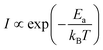 . An Ea significantly different from |ε0| is evidence for hopping-tunneling transition, |ε0| ≈ Ea pleads for a tunneling-throughout Sommerfeld–Arrhenius scenario.
(a2) with the value of the MO offset |ε1/2| obtained via ultraviolet photoelectron spectroscopy (UPS). Obviously, this makes sense in case of p-type conduction, where evidence exists that the “second” (tip) electrode negligibly affect the level alignment (ε1/2 ≈ ε0), which is basically the same for full and “half” (i.e. only SAM adsorbed on substrate without tip/top electrode) junctions.75,79,80 For n-type conduction determining the (LU)MO offset ε1/2via inverse photoelectron spectroscopy (IPS) could come into question.
(b) To start with a specific example, let us consider again the BCT junction of Section 7 and compare the ratio of the currents at room temperature and at liquid nitrogen IRT/ILN|V ≡ I(V,298.15 K)/I(V,77 K) computed using the exact eqn (7) for several biases V: IRT/ILN|V=1V = 11.38; IRT/ILN|V=0.9V = 5.55; IRT/ILN|V=0.8V = 2.20; IRT/ILN|V=0.7V = 1.31; IRT/ILN|V=0.6V = 1.10; IRT/ILN|V=0.5V = 1.05; IRT/ILN|V=0.4V = 1.03; IRT/ILN|V=0.4V = 1.02. These values show an almost exponential decrease in the thermal enhancement IRT/ILN in the narrow bias range 0.7 V ≲ V ≲ 1 V slightly below resonance (eVresonance = 2|ε0| ≃ 1.1 V). By contrast, sufficiently away from resonance (V ≲ 0.6 V) the thermal enhancement is practically negligible (IRT/ILN|V≲0.6V ≈1). This example illustrates that the Sommerfeld–Arrhenius transition is bias sensitive. In a given junction, a Sommerfeld–Arrhenius transition is observable at some biases while at other biases it cannot be observed. Such a bias sensitivity could not be expected if hopping dominated at higher temperature. The thermal activation energy is mainly determined by molecular properties (e.g., reorganization energy) which are little sensitive to external bias.
To sum up, by and large, data measured over a broad range of biases exhibiting a similar pattern (gradual transition between two distinct regimes) plead for a tunneling-hopping transition. Otherwise (i.e., if switching between a weak temperature dependence at low T to a strong T dependence at high T mainly occurs in a narrow range of V, see Fig. 11c) an overall tunneling picture applies; the temperature dependence is merely the result of thermally broadened Fermi distributions.
11 Conclusion
We hope that the various analytical formulas for the tunneling current reported here will assist experimentalists to adequately process transport data measured at nonvanishing (room) temperature and to more properly assign the transport mechanism at work in a specific molecular junction. Letting alone the aspect of elegance, the present analytical formulas have an important practical advantage over the often utilized brute force method of numerically integrating eqn (4) using a uniform energy grid. To resolve both the thermal smearing of the Fermi distributions and the variation of transmission with energy, a sufficiently fine uniform energy grid requires an energy step size δε ≈ min(kBT,Λ)/10. In an energy range Δε ∼ 10 eV this easily translates into a grid with N ∼ 104–106 points, which may make data fitting time consuming in some cases.
To be sure, adaptive numerical quadrature can alternatively be employed, and it is to be preferred to the brute force approach. Still, in spot checks to reproduce the present exact results obtained viaeqn (7), we had to conclude that applying adaptive numerical quadrature to eqn (4) with default settings (precision goal, working precision, etc.) using current distributions of MATHEMATICA (13.2.1) and MATLAB (R2021a) also poses nontrivial numerical problems for small Λ and kBT (kBT, Λ ≲ 1 meV).
Based on the results reported in this paper, for experimentalists unable to use eqn (7) to data fitting—e.g., because neither MATLAB nor ORIGIN can handle digamma function of complex argument—we recommend utilization of eqn (10g) and (9c), which provide a accurate description that complimentary covers most situations of practical interest. Albeit somewhat lengthy, they merely comprise elementary functions and can be used with any routine fitting software.
A cursory glance at an experimental curve looking like that depicted in Fig. 11d can easily be taken as “evidence” of a tunneling-hopping crossover or—in view of the T-dependent slope (“activation energy”)—of a variable variable-range hopping. In reality, we have seen that, it is the tunneling that is at work there both at low and high T. Emphasizing this point, the results reported above aim at aiding the molecular electronics community in not rushing conclude a transition from tunneling to hopping merely based on measured transport properties that switch from nearly temperature independent (Sommerfeld regime) to strongly temperature dependent (Arrhenius-like regime) upon rising the temperature.
The fact that the presently discussed Sommerfeld–Arrhenius can be tuned by bias can be an important theoretical finding in correctly assessing the physics underlying a curve like that of Fig. 11d.
Not to forget, we have also shown that the single level model considered in this paper is useful not only for single-molecule54,87,88 and CP-AFM69,75,79,89 junctions for which it was previously validated. It can also decipher charge transport in large area (n ≈ 500 μm2) junctions with EGaIn top electrode. For example, we have shown that, when adequately applied, even our off-resonant single level model43 can provide a reasonable estimate of the fraction of the current carrying molecules (f = Neff/Nn = eff/n ≈ 4 × 10⁻⁴) in a large area EGaIn junction fabricated with 1-tetradecanethiol.
Conflicts of interest
There are no conflicts to declare.
Acknowledgements
I am pleased to dedicate this paper to Professor Jochen Schirmer on the occasion of his 80th birthday and greatfully acknowledge fruitful interaction extending over many years. Financial support from the German Research Foundation (DFG Grant No. BA 1799/3-2) in the initial stage of this work and computational support by the state of Baden-Württemberg through bwHPC and the German Research Foundation through Grant No. INST 40/575-1 FUGG (bwUniCluster 2, bwForCluster/HELIX, and JUSTUS 2 cluster) are gratefully acknowledged.
References
- M. Poot, E. Osorio, K. O'Neill, J. M. Thijssen, D. Vanmaekelbergh, C. A. van Walree, L. W. Jenneskens and H. S. J. van der Zant, Nano Lett., 2006, 6, 1031–1035 CrossRef CAS.
- X. Li, J. Hihath, F. Chen, T. Masuda, L. Zang and N. Tao, J. Am. Chem. Soc., 2007, 129, 11535–11542 CrossRef CAS PubMed.
- S. H. Choi, B. Kim and C. D. Frisbie, Science, 2008, 320, 1482–1486 CrossRef CAS PubMed.
- H. Song, Y. Kim, Y. H. Jang, H. Jeong, M. A. Reed and T. Lee, Nature, 2009, 462, 1039–1043 CrossRef CAS PubMed.
- S. H. Choi and C. D. Frisbie, J. Am. Chem. Soc., 2010, 132, 16191–16201 CrossRef CAS PubMed.
- T. Hines, I. Diez-Perez, J. Hihath, H. Liu, Z.-S. Wang, J. Zhao, G. Zhou, K. Müllen and N. Tao, J. Am. Chem. Soc., 2010, 132, 11658–11664 CrossRef CAS PubMed.
- I. Diez-Perez, J. Hihath, T. Hines, Z.-S. Wang, G. Zhou, K. Müllen and N. Tao, Nat. Nanotechnol., 2011, 6, 226–231 CrossRef CAS PubMed.
- G. Sedghi, V. M. Garcia-Suarez, L. J. Esdaile, H. L. Anderson, C. J. Lambert, S. Martin, D. Bethell, S. J. Higgins, M. Elliott, N. Bennett, J. E. Macdonald and R. J. Nichols, Nat. Nanotechnol., 2011, 6, 517–523 CrossRef CAS PubMed.
- R. Heimbuch, H. Wu, A. Kumar, B. Poelsema, P. Schön, G. J. Vancso and H. J. W. Zandvliet, Phys. Rev. B: Condens. Matter Mater. Phys., 2012, 86, 075456 CrossRef.
- R. L. McCreery, H. Yan and A. J. Bergren, Phys. Chem. Chem. Phys., 2013, 15, 1065–1081 RSC.
- H. Yan, A. J. Bergren, R. McCreery, M. L. D. Rocca, P. Martin, P. Lafarge and J. C. Lacroix, Proc. Natl. Acad. Sci. U. S. A., 2013, 110, 5326–5330 CrossRef CAS PubMed.
- N. Amdursky, D. Ferber, I. Pecht, M. Sheves and D. Cahen, Phys. Chem. Chem. Phys., 2013, 15, 17142–17149 RSC.
- K. Asadi, A. J. Kronemeijer, T. Cramer, L. Jan Anton Koster, P. W. M. Blom and D. M. de Leeuw, Nat. Commun., 2013, 4, 1710 CrossRef PubMed.
- S. Saha, J. R. Owens, V. Meunier and K. M. Lewis, Appl. Phys. Lett., 2013, 103, 173101 CrossRef.
- Q. Ferreira, A. M. Bragança, L. Alcácer and J. Morgado, J. Phys. Chem. C, 2014, 118, 7229–7234 CrossRef CAS.
- O. E. Castañeda Ocampo, P. Gordiichuk, S. Catarci, D. A. Gautier, A. Herrmann and R. C. Chiechi, J. Am. Chem. Soc., 2015, 137, 8419–8427 CrossRef PubMed.
- L. Xiang, J. L. Palma, C. Bruot, V. Mujica, M. A. Ratner and N. Tao, Nat. Chem., 2015, 7, 221–226 CrossRef CAS PubMed.
- G. Pace, L. Caranzi, S. G. Bucella, G. Dell'Erba, E. Canesi, C. Bertarelli and M. Caironi, Nanoscale, 2014, 7, 2076–2084 RSC.
- M. Gilbert Gatty, A. Kahnt, L. J. Esdaile, M. Hutin, H. L. Anderson and B. Albinsson, J. Phys. Chem. B, 2015, 119, 7598–7611 CrossRef CAS PubMed.
- D. Taherinia, C. E. Smith, S. Ghosh, S. O. Odoh, L. Balhorn, L. Gagliardi, C. J. Cramer and C. D. Frisbie, ACS Nano, 2016, 10, 4372–4383 CrossRef CAS PubMed.
- C. S. S. Sangeeth, A. T. Demissie, L. Yuan, T. Wang, C. D. Frisbie and C. A. Nijhuis, J. Am. Chem. Soc., 2016, 138, 7305–7314 CrossRef CAS PubMed.
- Y. Li, L. Xiang, J. L. Palma, Y. Asai and N. Tao, Nat. Commun., 2016, 7, 11294 CrossRef CAS PubMed.
- L. Xiang, T. Hines, J. L. Palma, X. Lu, V. Mujica, M. A. Ratner, G. Zhou and N. Tao, J. Am. Chem. Soc., 2016, 138, 679–687 CrossRef CAS PubMed.
- R. L. McCreery, Beilstein J. Nanotechnol., 2016, 7, 32–46 CrossRef CAS PubMed.
- A. R. Garrigues, L. Yuan, L. Wang, E. R. Mucciolo, D. Thompon, E. del Barco and C. A. Nijhuis, Sci. Rep., 2016, 6, 26517 CrossRef CAS PubMed.
- A. R. Garrigues, L. Yuan, L. Wang, S. Singh, E. del Barco and C. A. Nijhuis, Dalton Trans., 2016, 45, 17153–17159 RSC.
- K. S. Kumar, R. R. Pasula, S. Lim and C. A. Nijhuis, Adv. Mater., 2016, 28, 1824–1830 CrossRef CAS PubMed.
- C. Jia, A. Migliore, N. Xin, S. Huang, J. Wang, Q. Yang, S. Wang, H. Chen, D. Wang, B. Feng, Z. Liu, G. Zhang, D.-H. Qu, H. Tian, M. A. Ratner, H. Q. Xu, A. Nitzan and X. Guo, Science, 2016, 352, 1443–1445 CrossRef CAS PubMed.
- D. Xiang, X. Wang, C. Jia, T. Lee and X. Guo, Chem. Rev., 2016, 116, 4318–4440 CrossRef CAS PubMed.
- N. Xin, C. Jia, J. Wang, S. Wang, M. Li, Y. Gong, G. Zhang, D. Zhu and X. Guo, J. Phys. Chem. Lett., 2017, 8, 2849–2854 CrossRef CAS PubMed.
- A. Morteza Najarian and R. L. McCreery, ACS Nano, 2017, 11, 3542–3552 CrossRef CAS PubMed.
- C. E. Smith, Z. Xie, I. Bâldea and C. D. Frisbie, Nanoscale, 2018, 10, 964–975 RSC.
- S. Valianti, J.-C. Cuevas and S. S. Skourtis, J. Phys. Chem. C, 2019, 123, 5907–5922 CrossRef CAS.
- N. Xin, C. Hu, H. Al Sabea, M. Zhang, C. Zhou, L. Meng, C. Jia, Y. Gong, Y. Li, G. Ke, X. He, P. Selvanathan, L. Norel, M. A. Ratner, Z. Liu, S. Xiao, S. Rigaut, H. Guo and X. Guo, J. Am. Chem. Soc., 2021, 143, 20811–20817 CrossRef CAS PubMed.
- S. Park, J. W. Jo, J. Jang, T. Ohto, H. Tada and H. J. Yoon, Nano Lett., 2022, 22, 7682–7689 CrossRef CAS PubMed.
- C. Caroli, R. Combescot, P. Nozieres and D. Saint-James, J. Phys. C: Solid State Phys., 1971, 4, 916 CrossRef.
- C. Caroli, R. Combescot, D. Lederer, P. Nozieres and D. Saint-James, J. Phys. C: Solid State Phys., 1971, 4, 2598 CrossRef.
- R. Combescot, J. Phys. C: Solid State Phys., 1971, 4, 2611 CrossRef.
- W. Schmickler, J. Electroanal. Chem., 1986, 204, 31–43 CrossRef CAS.
- I. R. Peterson, D. Vuillaume and R. M. Metzger, J. Phys. Chem. A, 2001, 105, 4702–4707 CrossRef CAS.
- C. A. Stafford, Phys. Rev. Lett., 1996, 77, 2770–2773 CrossRef CAS PubMed.
- M. Büttiker and D. Sánchez, Phys. Rev. Lett., 2003, 90, 119701 CrossRef PubMed.
- I. Bâldea, Phys. Rev. B: Condens. Matter Mater. Phys., 2012, 85, 035442 CrossRef.
- J. G. Simmons, J. Appl. Phys., 1963, 34, 1793–1803 CrossRef.
- I. Bâldea, Phys. Chem. Chem. Phys., 2015, 17, 20217–20230 RSC.
- I. Bâldea, Phys. Chem. Chem. Phys., 2017, 19, 11759–11770 RSC.
- I. Bâldea, Org. Electron., 2017, 49, 19–23 CrossRef.
- Z. Xie, I. Bâldea and C. D. Frisbie, Chem. Sci., 2018, 9, 4456–4467 RSC.
- I. Bâldea, Phys. Rev. B, 2021, 103, 195408 CrossRef.
- Z. Xie, I. Bâldea, Q. Nguyen and C. D. Frisbie, Nanoscale, 2021, 13, 16755–16768 RSC.
- I. Bâldea, Adv. Theory Simul., 2022, 5, 2200077 CrossRef.
- I. Bâldea, Adv. Theory Simul., 2022, 5, 202200158 Search PubMed.
- I. Bâldea, Int. J. Mol. Sci., 2022, 23, 14985 CrossRef PubMed.
- L. A. Zotti, T. Kirchner, J.-C. Cuevas, F. Pauly, T. Huhn, E. Scheer and A. Erbe, Small, 2010, 6, 1529–1535 CrossRef CAS PubMed.
-
H. J. W. Haug and A.-P. Jauho, Quantum Kinetics in Transport and Optics of Semiconductors, Springer Series in Solid-State Sciences, Berlin, Heidelberg, New York, second, substantially revised edn, 2008, vol. 123 Search PubMed.
-
G. D. Mahan, Many-Particle Physics, Plenum Press, New York and London, 2nd edn, 1990 Search PubMed.
- I. Bâldea, Phys. Chem. Chem. Phys., 2023, 25, 19750–19763 RSC.
-
I. Bâldea, Comment on “A single level tunneling model for molecular junctions: evaluating the simulation methods” by Opodi et al., 2023, Phys. Chem. Chem. Phys. 10.1039/D2CP05110A, ChemRxiv, preprint DOI:10.26434/chemrxiv-2023-7fx77.
-
K. Maki, in Superconductivity, ed. R. D. Parks, Dekker, New York, 1969, ch. Gapless Superconductivity, vol. 2, p. 1035 Search PubMed.
- I. Bâldea and M. Bădescu, Phys. Rev. B: Condens. Matter Mater. Phys., 1993, 48, 8619–8628 CrossRef PubMed.
- I. Bâldea, Adv. Theory Simul., 2022, 5, 2100480 CrossRef.
- L. E. Hall, J. R. Reimers, N. S. Hush and K. Silverbrook, J. Chem. Phys., 2000, 112, 1510–1521 CrossRef CAS.
- I. Bâldea and H. Köppel, Phys. Rev. B: Condens. Matter Mater. Phys., 2010, 81, 193401 CrossRef.
- I. G. Medvedev, J. Chem. Phys., 2017, 147(19), 194108 CrossRef PubMed.
-
Handbook of Mathematical Functions with Formulas, Graphs, and Mathematical Tables, ed. M. Abramowitz and I. A. Stegun, National Bureau of Standards Applied Mathematics Series, U.S. Government Printing Office, Washington, D.C., 1964 Search PubMed.
-
E. Jahnke and F. Emde, Tables
of Functions with Formulae and Curves, Dover Publications, 4th edn, 1945 Search PubMed.
-
A. Sommerfeld and H. Bethe, in Handbuch der Physik, ed. H. Geiger and K. Scheel, Julius-Springer-Verlag, Berlin, 1933, vol. 24(2), p. 446 Search PubMed.
-
N. W. Ashcroft and N. D. Mermin, Solid State Physics, Saunders College Publishing, New York, 1976, pp. 20–23, 52 Search PubMed.
- Z. Xie, I. Bâldea, A. T. Demissie, C. E. Smith, Y. Wu, G. Haugstad and C. D. Frisbie, J. Am. Chem. Soc., 2017, 139, 5696–5699 CrossRef CAS PubMed.
- C. M. Bowers, K.-C. Liao, T. Zaba, D. Rappoport, M. Baghbanzadeh, B. Breiten, A. Krzykawska, P. Cyganik and G. M. Whitesides, ACS Nano, 2015, 9, 1471–1477 CrossRef CAS PubMed.
- Y. Selzer, L. Cai, M. A. Cabassi, Y. Yao, J. M. Tour, T. S. Mayer and D. L. Allara, Nano Lett., 2005, 5, 61–65 CrossRef CAS PubMed.
- F. Milani, C. Grave, V. Ferri, P. Samori and M. A. Rampi, ChemPhysChem, 2007, 8, 515–518 CrossRef CAS PubMed.
- F. C. Simeone, H. J. Yoon, M. M. Thuo, J. R. Barber, B. Smith and G. M. Whitesides, J. Am. Chem. Soc., 2013, 135, 18131–18144 CrossRef CAS PubMed.
- S. Mukhopadhyay, S. K. Karuppannan, C. Guo, J. A. Fereiro, A. Bergren, V. Mukundan, X. Qiu, O. E. Castaneda Ocampo, X. Chen, R. C. Chiechi, R. McCreery, I. Pecht, M. Sheves, R. R. Pasula, S. Lim, C. A. Nijhuis, A. Vilan and D. Cahen, iScience, 2020, 23, 101099 CrossRef CAS PubMed.
- Z. Xie, I. Bâldea and C. D. Frisbie, J. Am. Chem. Soc., 2019, 141, 18182–18192 CrossRef CAS PubMed.
- A. T. Demissie, G. Haugstad and C. D. Frisbie, J. Phys. Chem. Lett., 2016, 7, 3477–3481 CrossRef CAS PubMed.
- H. J. Yoon, C. M. Bowers, M. Baghbanzadeh and G. M. Whitesides, J. Am. Chem. Soc., 2014, 136, 16–19 CrossRef CAS PubMed.
-
D. A. Papaconstantopoulos, Handbook of the Band Structure of Elemental Solids, Springer, 2nd edn, 2015 Search PubMed.
- Z. Xie, I. Bâldea, C. Smith, Y. Wu and C. D. Frisbie, ACS Nano, 2015, 9, 8022–8036 CrossRef CAS PubMed.
- Z. Xie, I. Bâldea and C. D. Frisbie, J. Am. Chem. Soc., 2019, 141, 3670–3681 CrossRef CAS PubMed.
- M. Paulsson and S. Datta, Phys. Rev. B: Condens. Matter Mater. Phys., 2003, 67, 241403 CrossRef.
- N. Mott and W. Twose, Adv. Phys., 1961, 10, 107–163 CrossRef CAS.
- R. M. Hill, Philos. Mag., 1971, 24, 1307–1325 CrossRef CAS.
- R. M. Hill, Phys. Status Solidi A, 1976, 34, 601–613 CrossRef CAS.
- H. Poole, London, Edinburgh Dublin Philos. Mag. J. Sci., 1916, 32, 112–129 CrossRef.
- J. Frenkel, Phys. Rev., 1938, 54, 647–648 CrossRef.
- I. Bâldea, J. Am. Chem. Soc., 2012, 134, 7958–7962 CrossRef PubMed.
- K. Luka-Guth, S. Hambsch, A. Bloch, P. Ehrenreich, B. M. Briechle, F. Kilibarda, T. Sendler, D. Sysoiev, T. Huhn, A. Erbe and E. Scheer, Beilstein J. Nanotechnol., 2016, 7, 1055–1067 CrossRef CAS PubMed.
- A. Tan, S. Sadat and P. Reddy, Appl. Phys. Lett., 2010, 96, 013110 CrossRef.
|
| This journal is © the Owner Societies 2024 |
Click here to see how this site uses Cookies. View our privacy policy here. 

 is the Fermi–Dirac distribution, and μs,t = ±eV/2 are the chemical potentials of the electrodes (“substrate s and “tip/top” t).


 . Using again the definition of r1, we deduce
 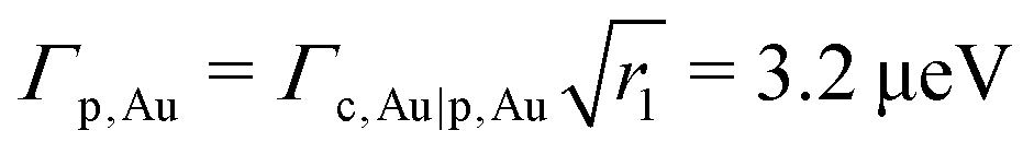 . From the definition of r2 of eqn (14b) we get Γp,EGaIn = r2Γp,Au = 0.456 μeV. From eqn (14a) we can now compute
 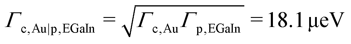 . With the value Σ = 3.5 mol nm−2 measured for the molecular coverage of alkanethiol SAMs,76 and the fitting parameter value
 using the low bias conductance G obtained from the slope of the measured I–V curve at low bias. With the values of ε0, Γ and γ thus obtained compare the measured curve with the simulated curve computed using our eqn (8b) in the bias range −1.2|Vt−| ≲ V ≲ 1.2Vt+. Alternatively, always in the bias range indicated (for which eqn (8b) applies), one can fit the measured data to I0K-off of eqn (8b) wherein ε0, Γ and γ are adjustable parameters. (ii) If attempt (i) fails to produce a good theoretical curve, fit data to I0K of eqn (8a) in the entire bias accessed experimentally with ε0, Γ, γ, and Λ as adjustable parameters. If the corresponding point (ε0K0, Λ0K) falls in the colored regions of Fig. 6a, 7a, 8a or 9a, this is evidence that the best fit values ε0K0, Γ0K, γ0K and Λ0K are reliable and that, at the corresponding bias, eqn (8a) is reliable. In other words, at the envisaged bias, thermal corrections to the current are negligible. Notice that (like eqn (8b) and (8a)) can hold up to a certain bias (e.g., V = 0.5 V) but can become inadequate at higher biases (e.g., V = 1 V) (see the example of Section 7). (iii) The failure of attempt (ii) indicates that (possibly only beyond certain biases) the temperature dependence of the current is significant. Generally speaking, whenever possible (e.g., using MATHEMATICA) fitting data to the exact eqn (7) is then most advisable. Otherwise the various analytical formulas for the current Il,1, Il,2, Il,2 of eqn (9) or Ih,1, Ih,2 of eqn (10) can be easier applied. Because they merely contain elementary functions the approximate formulas for Il,1, Il,2, Il,2, Ih,1, and Ih,2 are implementable in any fitting software package. Loosely speaking, the deeper the point (ε0K0, Λ0K) into the white (non-colored) regions mentioned under (ii) above, the stronger is the impact of T on the current at the corresponding bias. (iiia) For cases wherein the point (ε0K0, Λ0K) lies near the edge between colored and non-colored regions of Fig. 6a, 7a, 8a, or 9a, thermal effects are rather weak, and using the formula of Il,1 of eqn (10g) for data fitting is advisable. If the best fitting point (εl,10, Λl,1) obtained fitting the experimental I–V curve to eqn (10h) is found in the colored regions of Fig. 6b, 7b, 8b, or 9bIl,1 provides an accurate description and the fitting parameters εl,10, Γl,1, γl,1, and Λl,1 are good estimates of the corresponding quantities. Otherwise, performing and inspecting the results of data fitting based on Il,2 of eqn (9c) (and then Il,3 of eqn (9d) if the case) follows in the next step. (iiib) If the point (ε0K0, Λ0K) lies deep inside the white (non-colored) regions of Fig. 6a, 7a, 8a, or 9a, thermal effects are strong, and the formula deduced via high temperature expansions (Ih,1 of eqn (10g)) and Ih,2 of eqn (10h) should be employed for reliably estimate the parameters ε0, Γ, γ, and Λ for the junction under investigation. In cases where (iiib) applies, performing I–V measurements at variable temperature is highly desirable, and the issues related to the Sommerfeld–Arrhenius transition addressed in the next section deserve consideration.
 at high T due to thermally activated hopping or evidence for the strongly T-dependent tunneling current discussed in this paper? To differentiate between these two possibilities, in previous studies we suggested investigations of junctions having electrodes with significantly different work function32,46 or subject to mechanical stretching.53 The present results indicate two alternatives easier to implement experimentally in order to differentiate between strongly T-dependent tunneling and hopping: (a) To unravel the physics underlying an observed switching from strong T-dependent to T-independent (or weak T-dependent) currents, I–V curves measured at low temperatures can be fitted to eqn (8) assuming T-independent I (or eqn (9) assuming weak T-dependent I). The value |ε0| of the MO offset thus obtained can be compared:
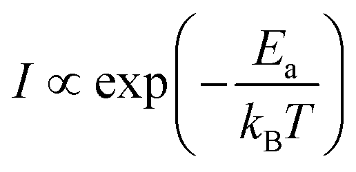 . An Ea significantly different from |ε0| is evidence for hopping-tunneling transition, |ε0| ≈ Ea pleads for a tunneling-throughout Sommerfeld–Arrhenius scenario.