
 Open Access Article
 This Open Access Article is licensed under a Creative Commons Attribution-Non Commercial 3.0 Unported Licence
A density-matrix adaptation of the Hückel method to weak covalent networks
Laura
Van Dorn
 and
Andrei
Sanov
*
and
Andrei
Sanov
*
Department of Chemistry and Biochemistry, The University of Arizona, Tucson, Arizona 85721, USA. E-mail: sanov@arizona.edu
First published on 29th January 2024
Abstract
The coupled-monomers model is built as an adaptation of the Hückel MO theory based on a self-consistent density-matrix formalism. The distinguishing feature of the model is its reliance on variable bond and Coulomb integrals that depend on the elements of the density matrix: the bond orders and partial charges, respectively. Here the model is used to describe electron reactivity in weak covalent networks Xn±, where X is a closed-shell monomer. Viewing the electron as the simplest chemical reagent, the model provides insight into charge sharing and localisation in chains of such identical monomers. Data-driven modelling improves the results by training the model to experimental or ab initio data. Among key outcomes is the prediction that the charge in Xn± clusters tends to localise on a few (2–3) monomers. This is confirmed by the properties of several known cluster families, including Hen+, Arn+, (glyoxal)n−, and (biacetyl)n−. Since this prediction is obtained in a purely coherent covalent regime without any thermal excitation, it implies that charge localisation does not require non-covalent perturbations (such as solvation), decoherence, or free-energy effects. Instead, charge localisation is an intrinsic feature of weak covalent networks arising from their geometry relaxation and is ultimately attributed to the correlation between covalent bond orders and equilibrium bond integrals.
1. Introduction
The electron is the simplest chemical reagent. Chemistry can be initiated in a variety of ways, but ultimately it is electron movements that make or break chemical bonds. Electron reactivity is, therefore, central to understanding the molecular universe.Here we consider the interactions of electrons with ensembles of closed-shell atoms or molecules. These interactions may rely on a variety of covalent or non-covalent1–7 forces, but in this work we examine charge capture by valence orbitals only. The injection of a single electron or electron hole leads to radicalisation of monomers that were non-reactive in the neutral state. The resulting reactivity raises an important issue in both chemistry and physics: that of coherent charge sharing versus localisation.
Charge sharing is responsible for covalent bonding. We set out to investigate how many identical closed-shell monomers can bind a single bonding agent (an electron or hole) in their valence orbitals in a perturbation- and excitation-free regime. We are especially interested in the physical factors that determine if the charge is localised on a few monomers or shared by many moieties,8–10 perhaps resembling (in size only) the diffuse non-valence states of solvated electrons.11–19
We approach charge sharing using an extension of the classic Hückel molecular orbital (MO) theory20–25 combined with the correlation between bond energy and bond order26 that has long been ubiquitous in the literature.27–39 True to its predecessors’ spirit, our straightforward model emphasises physical insight over the precision and complexity of higher-level ab initio theory.40,41 The presented model is intended to be highly trainable, to borrow a term from machine learning,42 meaning its performance can be significantly improved using either experimental or ab initio data. The objective of the training process is not just to match known data but to provide a translation of results into their physical meaning in terms of common chemical concepts. The aspirational value of this approach is similar to that of the original Hückel theory, which remains relevant today, in the age of computers and high-accuracy ab initio calculations.
We first turn to the classic dimer anion of CO2,43 the core of some (CO2)n− clusters.44–48 In this dimer, the excess electron resides in an inter-monomer orbital (IMO), which is a bonding superposition of the lowest vacant orbitals of two CO2 moieties, each distorted by the partial negative charge into a bent geometry.43 An unpaired electron populating the IMO creates an inter-monomer (IM) bond with a nominal order of 1/2 joining the two CO2 moieties in a weakly bonded −1/2(O2C)–(CO2)−1/2 structure.
Similar anionic dimers can form from other closed-shell species. For example, the recent photoelectron spectra of the biacetyl (ba) cluster anions suggested the existence of covalent bonding between the two ba moieties in the ba2− dimer anion,49 similar to the bonding motif in (CO2)2−. This conclusion was supported by theory calculations indicating that the IM bonding in ba2− is the result of an electron entering an IMO comprised of the low-lying π LUMOs of the monomers. A similar structure was also predicted for the dimer anion of glyoxal (gl).9
Dimer examples also exist for positive ions, starting with the rare-gas dimer cations He2+, Ne2+, and Ar2+, and others.50–56 As predicted by basic MO theory, the bonding in these species is due to an electron removed from the respective anti-bonding IMOs defined as superpositions of s (for He) or p (for others) ![[m with combining low line]](https://www.rsc.org/images/entities/char_006d_0332.gif) onoer
onoer ![[o with combining low line]](https://www.rsc.org/images/entities/char_006f_0332.gif) rbitals (MMO). An anti-bonding electron orbital becomes bonding if populated by holes, and vice versa. Therefore, the bond formation in these dimers can be described as removal of an order-of-1/2 anti-bond, creating an equivalent half-bond.
rbitals (MMO). An anti-bonding electron orbital becomes bonding if populated by holes, and vice versa. Therefore, the bond formation in these dimers can be described as removal of an order-of-1/2 anti-bond, creating an equivalent half-bond.
Also of note are the dimer cations of benzene,57 uracil,58 adenine, and thymine59 studied by Krylov, Bradforth, and co-authors. In these systems, an IM bond is similarly created by removing an electron from an anti-bonding cluster orbital described as a superposition of benzene HOMOs (MMOs, using the above abbreviation). The authors fittingly referred to these cluster orbitals as dimer molecular orbitals,57 and it is only because our discussion extends beyond dimers that we use the more general term defined above, the inter-monomer orbital (IMO).
All the examples so far have basic bonding features in common. Each possesses an order-of-1/2 covalent bond between the monomers due to a single bonding agent (an electron for anions or a hole for cations) populating a cluster IMO described as a superposition of appropriate MMOs. There is, however, an important distinction between the LUMO of CO2 and all other MMOs mentioned. CO2 stands out because the bending upon addition of negative charge6,60–64 gives its MMO a predominantly monodirectional C sp2 character. It works well for a head-to-head overlap in the (CO2)2− structure43 but is not conducive to effective electron sharing among more than two monomers.8
In contrast, the bidirectional (π, p) or spherical (s) nature of all other MMO examples is amendable to stacking into longer chain structures, and trimer ions do exist among the already mentioned Hen+, Nen+, Arn+, gln−, and ban− cluster families.9,50,51,55,56,65–69 All have been subjects of high-level studies, and in all cases the most stable trimer structures correspond to covalently bonded X3± chains, where X is a closed-shell neutral monomer. For example, the He3+ and Ar3+ IMOs (specifically, the Hartree–Fock β-spin LUMOs computed in QChem70 for CCSD/aug-cc-pVTZ optimised structures) are plotted in Fig. 1(a) and (b), respectively. Comparing them to their constituent 1s or 3p MMOs (same figure, left), makes it clear that these trimer orbitals can indeed be described in terms of stacked MMOs. Similar side views of the gl−vs. gl3− and ba−vs. ba3− structures along with the respective MMOs and IMOs (the Kohn–Sham α-HOMOs)8,9,49 are shown in Fig. 1(c) and (d). Interestingly, no evidence of covalent trimer cations has been reported for benzene or other similar organics.57–59 Although π stacked trimer structures can be easily envisaged for these monomers, their stability is another matter.
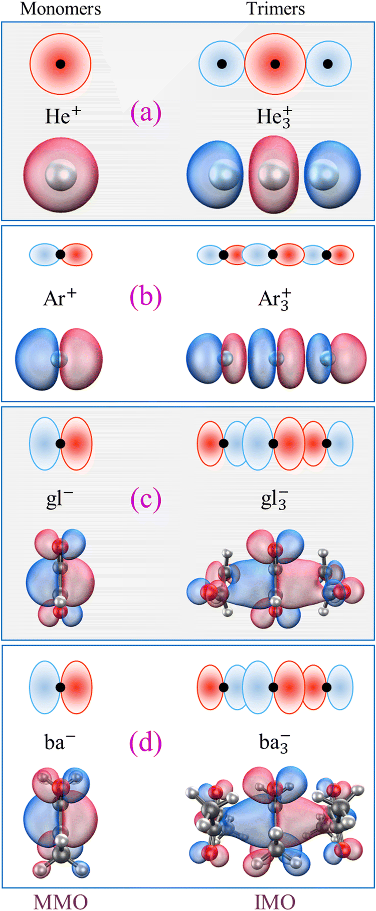 | ||
| Fig. 1 Left: The monomer orbitals (MMOs) of X = (a) He, (b) Ar, (c) glyoxal (gl), and (d) biacetyl (ba). Right: The inter-monomer orbitals (IMOs) of the respective X3± trimer ions. The orbitals shown in the bottom half of each panel are from ab initio or density-functional calculations referenced in the text. The top sketches are schematic depictions of these orbitals, emphasising the essential s, p, or π (p-like) characters and parity along the interaction axis. | ||
All trimer structures in Fig. 1 have similar overall properties. The monomers in each case are arranged in a linear (not triangular) (X–X–X)± geometry. For He3+, the linear structure is predicted by a simple Hückel calculation, while for the others it is dictated by the MMO shapes. In the Lewis structures of these trimers, each IM bond has a nominal order of 1/4 (one bonding electron or hole shared between two bonds). That said, the nominal bond orders should not be confused with the Hückel (or Coulson) mobile bond orders,25,71 and it is the latter that this work relies upon.
The question arises: is it possible for an electron or hole to be shared by the valence orbitals of a larger number of monomers? It seems that MMO stackability should enable the formation of electronically coherent Xn± chains held together by one delocalised bonding agent. Coherence implies a fixed phase relationship between the MMOs, which is a prerequisite for the IMO definition and covalent bonding. Without outside perturbations (such as solvation, vibronic couplings, or thermal effects), long Xn± chains would present fantastic case studies of electronic coherence and quantum wires.72 Alas, while all MMOs in Fig. 1 are infinitely stackable along the interaction axis, covalently bonded Xn± ions larger than trimers, with few exceptions,51 are not observed in these cluster families. Hen+ and Arn+ with n > 3 predominantly contain trimer–ion cores. For X = gl and ba, stable tetramer chain structures can be created by computational methods, but only under a symmetry constraint.9 If unconstrained, the charge in X4± tends to localise on a trimer core, with an additional mostly neutral monomer solvating the core ion. In sum, the dominant structures of Xn±, n ≥ 3 clusters, where X is a closed-shell monomer with a stackable MMO, are described as Xk±·Xn−k, where k ≤ 3.
Since the empirical trimer limit appears to be applicable to both negative and positive ions and to monomers with varying properties, its existence suggests a commonality of electron/hole reactivity that transcends the intrinsic chemistry of the monomers. It must reflect the general features of inter-monomer networking. Hence one of the questions we aim to answer: what is special about trimers?
We use this question as a test case for the coupled-monomers model described in this work. The results show that under a wide range of realistic assumptions, Xn± chains are unstable beyond the trimer. And for a rather simple reason, which has nothing to do with decoherence, solvation, or entropic contributions to free energy. To be sure, the competition between covalent bonding and solvation often favours certain ion core structures and is responsible for core-switching in several known cluster families.44,45,73–90 But it does not control the above trimer limit. To prove this, we will demonstrate this limit in a perfectly coherent, excitation-less regime excluding any non-covalent forces. Its true origin, rooted in the energetics of weak covalent interactions, will become apparent as an analysis outcome.
To examine the limits of charge sharing in weak covalent interactions, let us first consider what we call the Hückel reference. Its definition is given in Section 2, but briefly it refers to a chain of identical closed-shell monomers X interacting with a single bonding agent under the approximations of the original Hückel MO theory.
The key feature of the Hückel reference is the unobstructed charge delocalization over the entire Xn± chain. This is illustrated in Fig. 2 on the example of an n = 9 chain defined in (a). The filled blue symbols in (b) represent the amplitudes |ci| of the monomers’ contributions to the Xn± ground state obtained by diagonalising the Hückel Hamiltonian matrix with constant bond integrals Hi,i+1 = β for all nearest neighbours and zeros for others. The discrete Hückel solution overlaps with the continuous wave function of the particle-in-a-box ground state, shown by the dashed curve in the same figure.
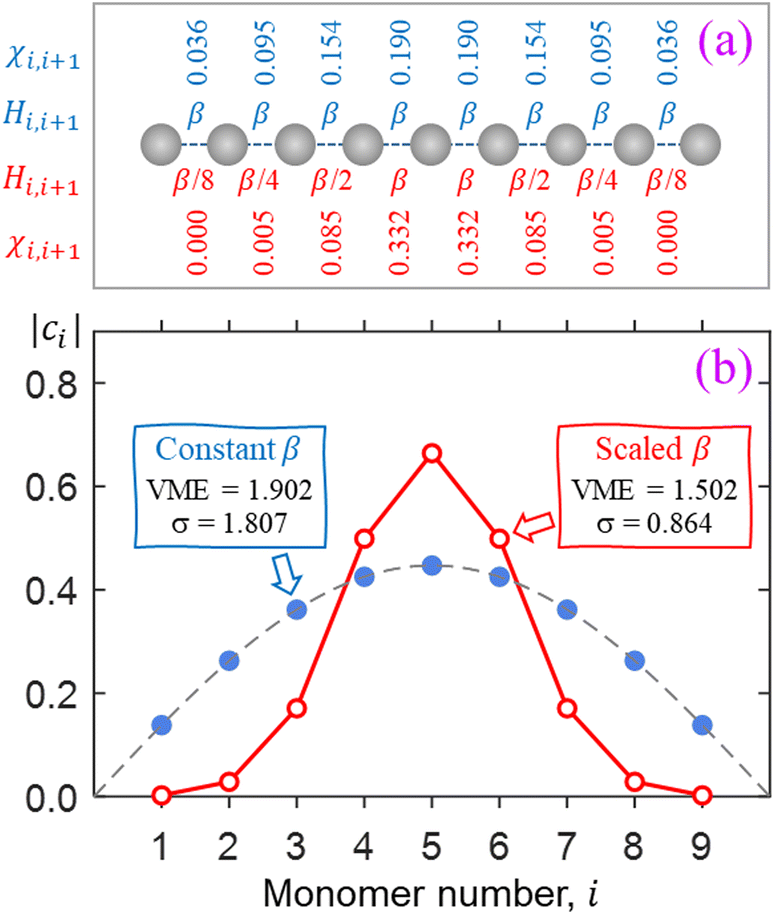 | ||
| Fig. 2 (a) Two model Xn±, n = 9, chains. Shown at the top in blue are the constant bond integrals Hi,i±1 = β and the resulting ground-state absolute bond orders (χi,i±1) of the Hückel reference. Below, in red, are the scaled bond integrals and bond orders of the second, non-Hückel model. (b) Blue and red symbols: the lowest-energy IMO amplitudes obtained by diagonalising the Hückel and scaled (non-Hückel) Hamiltonian matrices for the respective chains defined in (a). Dashed curve: the continuous ground-state wave function of the particle in a box representing the chain. | ||
The above IMO amplitudes result in absolute Hückel bond orders25,71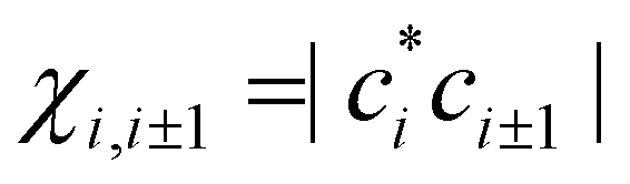 which decrease toward the ends of the chain. They are indicated at the top of Fig. 2(a) in blue font. In a real molecular chain, the variable bond orders will result in variable bond lengths: the weaker the bond, the longer it is. The lengthening of the bonds toward the ends of the chain is not considered in the Hückel model, but in the real world it will cause decreasing magnitudes of the corresponding bond integrals.
For a simple illustration, consider now a similar X9± chain but with the bond integrals progressively scaled by 1/2 for each bond toward either end of the chain. That is, instead of all Hi,i±1 = β, we will now assume scaled Hi,i±1 values of β/8, β/4, β/2, β, β, β/2, β/4, β/8, as shown below the model chain in Fig. 2(a) using red font. The IMO amplitudes corresponding to the lowest eigenvalue of the resulting H matrix are plotted using red open circles in Fig. 2(b). This solution represents a significant narrowing of the charge distribution compared to the Hückel reference. Specifically, 94% of the charge is now localised on the three middle monomers, compared to Hückel reference's 56%.
The scaling of the bond integrals in the above example was chosen arbitrarily. In the rest of this work, we hypothesise a quantitative relationship between bond integrals and the corresponding bond orders. We then calibrate this hypothesis using data for real chemical systems. It should be noted that our main qualitative conclusion is already apparent in Fig. 2, where charge localisation to a small subset of monomers is traced to the cluster's geometric response to bond-order variation.
Table 1 summarises the data for four Xn± families that we will use to guide the model training: X = He,50,55,66,67 Ar,50,56,68 gl,9 and ba.9 Included are the vertical monomerization energies (VME) of the dimer and trimer ions. Under the Hückel approximations, the trimer VME must be  times larger than the corresponding dimer bond energy.8 Yet in most cases, X = ba notwithstanding (vide infra), the dimer-to-trimer VME increase is smaller than the Hückel prediction. Consistent with Fig. 2, this is because the sharing of a single bonding agent between two trimer bonds results in a weakening and thus lengthening of these bonds, which in turn dampens the bond integrals.
| X = | He | Ar | gl | Hückel | ba |
|---|---|---|---|---|---|
| VME(2)/eV | 2.448 | 1.366 | 1.088 | 1.020 | |
| VME(2)/d.u. | 1 | 1 | 1 | 1 | 1 |
| VME(3)/eV | 2.598 | 1.567 | 1.324 | 1.583 | |
| VME(3)/d.u. | 1.061 | 1.147 | 1.217 | 1.414 | 1.552 |
As we seek a description of IM couplings in Xn± chains, the desired theory must include the geometry and (consequently) bond-integral relaxation in response to variable bond orders. This requirement makes the original Hückel MO theory not suitable for the task but does not imply that a rigorous application of the full MO theory is the only answer. The IM bonds resulting from a single bonding agent all have bond orders of ≤1/2, leading to relatively large equilibrium bond lengths. In this regime, significant simplifications of the MO theory are possible, giving rise to the model formalism described in the next section.
2. The coupled-monomers model
The presented model is a version of the general MO theory adapted to the requirements of weakly-bonded networks. Although many of the assumptions are the same as in the Hückel theory, our model features additional adaptivity with regard to the bond and Coulomb integrals. The flexible treatment of these parameters allows the model to be trained to describe the properties of specific systems. In this section, we spell out both the parallels and distinctions between the coupled-monomers model and the original Hückel MO theory.2.1. Model assumptions and formalism
Approximation 1: separation of IM interactions from intra-monomer bonding. We adopt a hierarchical approach that treats the IM interactions as perturbations of the monomers. Under this approximation, the intermonomer orbitals are described as linear combinations of unmodified monomer orbitals, one MMO per monomer. The MMOs used are the lowest-energy orbitals with a vacancy for an electron or hole, as appropriate.8,9Formally, in a system of n identical closed-shell monomers X, let ψi be the normalised MMO of X(i), i = 1,…, n. The set of n MMOs {ψi} serves as a minimal basis for describing the IM interactions in Xn upon the addition of an electron or hole.
Approximation 2: the model Hamiltonian. An electron/hole added to the IMO system spanned by the {ψi} basis is described by an effective Hamiltonian Ĥ, which incorporates the effects of all other electrons and the nuclei in an averaged way.25 Like in the Hückel method, we will avoid expressing the Hamiltonian in an explicit operator form and are not concerned with its details. The IMOs  and their energies Ek, k = 1,…,n are obtained from the secular equation for the H matrix representing Ĥ in the {ψi} basis. As in the LCAO-MO theory,25 the solutions generally depend on the H matrix elements, Hi,j = 〈ψi|Ĥ|ψj〉, and the overlap integrals Si,j = 〈ψi|ψj〉.
Approximation 3: basis set orthogonality. Like the Hückel method,20–25 we will treat the MMO basis as orthonormal by setting Si,j = δi,j (Kronecker's delta).
The relative weakness of the covalent couplings considered here results in large equilibrium bond lengths, making this assumption more robust than in a typical Hückel case. The secular equation then simplifies to an eigenvalue problem for H (only). It yields n eigenvalues Ek and the corresponding eigenvectors |ϕk〉 that contain the  coefficients (k = 1, …, n). Focusing on the most stable state, we select the lowest-energy IMO, ϕ = ϕ1, and hereafter drop index k = 1 for brevity. The energy of
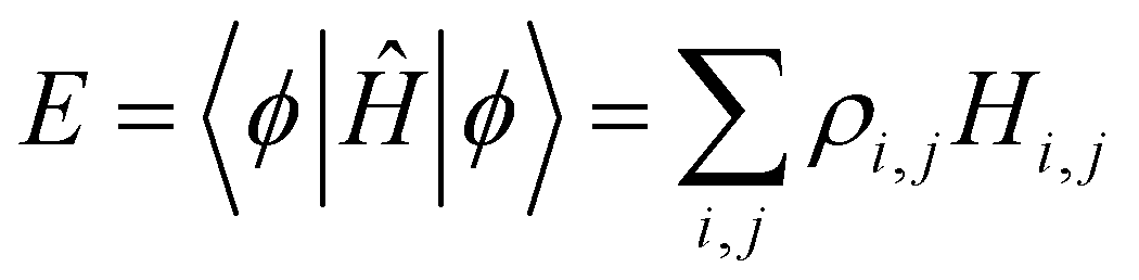
  is its eigenvalue E. Alternatively, it can be calculated from the density matrix ρ = |ϕ〉〈ϕ| as follows:
 | (1) |
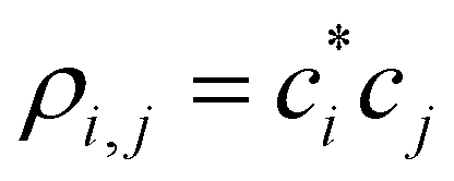 are the density matrix elements. Each diagonal element ρi,i is the electron (hole) density on X(i), i.e., the absolute partial charge of the monomer: ρi,i = qi. The off-diagonal elements ρi,j, i ≠ j are the Hückel (Coulson) bond orders.25
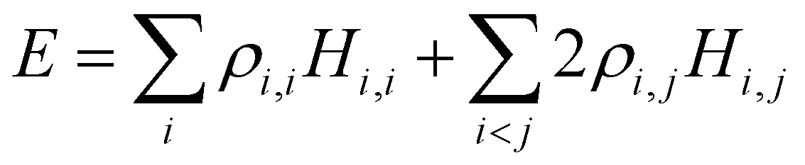
Separating the individual monomer contributions from pairwise interactions and counting the IM bonds rather than distinct i,j and j,i exchange pairs, it is convenient to rewrite eqn (1) as:
 | (2) |
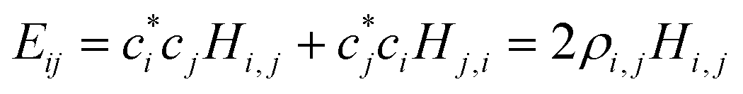 , i < j (for real Hi,j). It can be said that each Hi,j, i < j coupling constant is activated by the addition of an electron (hole), with a twice-the-bond-order (2ρi,j) weight.
Approximation 4.0: constant Coulomb integrals. Following Hückel,20–25 here we treat all Coulomb integrals Hi,i as constants, which are the same for all identical monomers: Hi,i = α. A constant α does not affect the bond energies (see below) and can be set arbitrarily to zero.
The effect of IM interactions in Xn± is conveniently expressed in terms of vertical monomerization energy (VME), which is defined as the energy change in the Xn± → X± + (n − 1)X process, excluding any internal monomer relaxation (hence ‘vertical’).8,9 Bonding and anti-bonding interactions contribute to VME with positive and negative signs, respectively, and it is positive overall for a bound system.
The VME of Xn± is obtained by subtracting the IMO energy from that of the charge localised on an isolated monomer, i.e., the Coulomb integral:
| VME = α − E | (3) |
 , since
 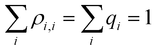 . Substituting the simplified eqn (2) into eqn (3), we get:8
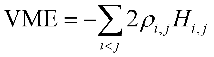 | (4) |
The Hückel-like assumption of α = const is oversimplistic in many chemical scenarios, and in a follow-up paper we will replace the α constant with a variable α function, α(q), where q is the absolute charge of the monomer, qi = ρi,i. That is, Hi,i = α(qi). We will refer to the assumption of an α-function instead of an α-constant as approximation 4.1. One of its immediate consequences is that it invalidates eqn (4).
The Hückel reference
The Hückel model for any Xn± structure is obtained by setting all Coulomb integrals to a constant α and all bond integrals to a constant β for connected monomers and to zero for all remote pairs.25 In this work, we refer to any Xn± structure described in these terms as the Hückel reference.A discussion of the Hückel reference for anionic arrays in one to three dimensions was presented elsewhere.8 Importantly, the Hückel structures exhibit a particle-in-a-box-type charge delocalisation.8,9,25 Stabilisation due to one electron (hole) entering the lowest-energy IMO is given by VME(2) = |β| for the dimer and  for the trimer. For n > 3, VME(n) continues to increase but saturates at VME(n) → 2|β| for n → ∞.8 This limit is also due to the particle-in-a-box behaviour. As the chain (box) length increases, the ground-state eigenvalue E decreases but remains bounded from below by the bottom of the box. Per eqn (3), this restriction puts an upper bound on VME(n).
The assumption of constant bond integrals works well in the Hückel theory's original domain where π electrons are added to a framework of σ bonds in conjugated hydrocarbons. Although the σ bonds are not part of Hückel's original formalism, they dictate a robust structure within which the π bond integrals are defined. The constant β assumption is also acceptable for systems with other types of equivalent bonds (e.g., the triangular structure of H3+). However, it becomes problematic if the entirety of the bonding being considered is due to the added electron (hole) and the bonds in questions are fundamentally not equivalent.8,9
To this point, the IM bonds in clusters like Hen+ and ban− are not added to any pre-existing IM bonding framework (excepting the weak van der Waals forces); they alone define the IM bonding structures. In this scenario, the bond lengths and hence the bond integrals vary significantly from one bond to another, and any model keeping them constant will miss essential chemistry. We are, therefore, compelled to treat Hi,j, i ≠ j as explicit functions of IM geometry.
Approximation 5: the bonding function. The bond integral Hi,j = 〈ψi|Ĥ|ψj〉, i ≠ j explicitly depends on the distance between the monomers, Ri,j. Focusing on the nearest-neighbour interactions only, we express the bond integrals Hi,i±1 in Xn± chains using an explicit function of bond length,
| Hi,i±1 = H(Ri,i±1) | (5) |
Eqn (5) applies to any bond length, but we are interested in relaxed ground-state structures. Labelling the equilibrium Ri,i±1 as ri,i±1 and the corresponding matrix elements Hi,i±1 as hi,i±1, the bond integrals in a relaxed structure are defined, per eqn (5), as hi,i±1 = H(ri,i±1).
The relaxed bond lengths, in turn, depend on the bond orders. Hence, we postulate ri,i±1 = r(χi,i±1), where χi,i±1 is the order of the bond between adjacent monomers i and i ± 1 and r(χ) is a function. To make this function independent of the basis set parity, its argument χ = χi,i±1 is defined as the absolute, not Hückel, bond order. “Absolute” as used here does not mean that χ is always positive, but that it is positive for bonding interactions and negative for anti-bonding, independent of the basis set. Depending on the basis MMOs’ relative phases and the nature of the bonding particles (electrons or holes), χi,i±1 may differ in sign from the Hückel bond orders 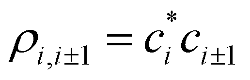 (more on this in a future paper). Specifically, for bonding interactions, χi,i±1 = |ρi,i±1| > 0 and r(χi,i±1) is finite, with r(χ) → ∞ for χ → 0. For antibonding, χi,i±1 = −|ρi,i±1| < 0 and r(χ) is infinite for χ ≤ 0.
It follows that the equilibrium values of bond integrals vary with absolute bond orders because hi,i±1 = H(ri,i±1) = H[r(χi,i±1)], or, equivalently,
| hi,i±1 = β(χi,i±1) | (6) |
Following the convention of the original Hückel method, we will assume that the {ψi} MMO basis set is defined in such a way that all nearest-neighbour bond integrals hi,i±1 are negative, corresponding to a bonding overlap of each pair of adjacent basis functions. In such a basis, per eqn (6), β(χ) is a negative-valued function like Hückel's original β constant.
2.2. Self-consistent solutions
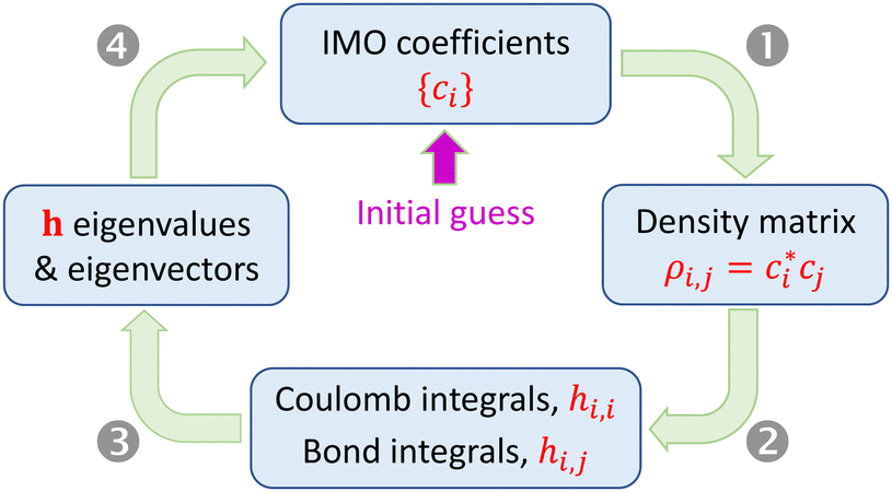
Under the approximations in Section 2.1, the Hamiltonian matrix elements hi,j for a relaxed Xn± chain can be determined from the density matrix elements ρi,j. For that, we need the bonding function β(χ) and the Coulomb-integral constant α (or, more generally, the α-function). Diagonalizing matrix h yields the IMOs and their eigenvalues. However, the dependence of hi,j on sets up a circular problem: since ci are the eigenvector coefficients, the problem's statement (hi,j) depends on its own solution ({ci}). This difficulty is resolved by an iterative search for a self-consistent solution using the algorithm shown in Fig. 3.
 | ||
| Fig. 3 Search for self-consistent solutions. Details in the text. | ||
A calculation is initiated with an arbitrary guess of the initial state in the |ϕ〉 vector space, defined by a set of the initial IMO coefficients, {ci}. Each iteration includes the following steps:
(1) From the current {ci}, compute the density matrix elements,  . The diagonal elements ρi,i are the MMO (ψi) populations, while all others are the i,j bond orders.
(2) (a) Set all Coulomb integrals to the same constant (e.g., zero), per approximation 4.0. Alternatively, variable Coulomb integrals can be calculated as hi,i = α(ρi,i) (approximation 4.1). (b) Evaluate the nearest-neighbour bond integrals from the bond orders using eqn (6) with an assumed or otherwise known bonding function (approximation 5). In the Xn± ground state, all nearest-neighbour interactions are bonding, so the absolute bond orders are obtained from the density matrix as χi,i±1 = |ρi,i±1|. (c) Set all remote integrals Hi,j, |i − j| > 1, to zero.
(3) Find the eigenvalues and eigenvectors of matrix h from the previous step.
(4) Calculate VME from the lowest h eigenvalue per eqn (3). If α = const, eqn (4) gives the same result. Check for convergence and proceed to the next iteration (Step 1) or exit the loop.
The convergence check included two criteria, both of which had to be satisfied to complete the calculation. First, the change in the energy eigenvalue relative to the previous iteration must be <10−6 dimer units (Section 2.3). Second, the norm of the corresponding change of the eigenvector must be <10−7. Depending on the initial guess, most calculations involved <100 iterations. Some were <10, but a few required >1000 iterations to converge. The computing times are generally minimal. The longest calculation attempted involved 104 monomers (108 matrix elements), requiring 42 iterations and less than 2 min of wall time to converge on a modest 2.5 GHz processor with 32 GB of RAM.
2.3. The dimer units
In an Xn± system bonded by one electron (hole), the equilibrium bond integrals hi,i±1 and hence β(χ) have the largest magnitude for χ = 0.5, which is the maximum absolute bond order attributable to one electron or hole. This limit is achieved when the electron (hole) is localized on a single bond, i.e., in an X2± dimer.Therefore, we will refer to χ = 0.5 as the dimer limit and define the corresponding bond energy, VME(2) = |β(0.5)|, as the dimer unit (d.u.) of energy. It follows that β(0.5) = −1 d.u. by definition. For example, given that the monomerization energy of He2+ is VME(2) = 2.448 eV, while that of He3+ is VME(3) = 2.598 eV (Table 1),50,55,66,67 it follows that the dimer unit of energy for the Hen+ cluster family is 1 d.u. = 2.448 eV and the total stabilisation energy of the trimer is 1.061 d.u.
So defined, the dimer units are explicitly system (X) dependent, and that is the point. This definition is meant to take the focus off the differences between monomers and instead facilitate the comparison of the n dependent trends in various Xn± families. The key benefit of this approach is that it allows the presentation of results in a universal, X-independent language.
2.4. The empirical bonding function
Before exploring the properties of the bonding function, we consider its universal properties.The χ = 0 boundary corresponds to the non-bonding limit. As χ → 0, we expect the equilibrium bond length to tend to infinity and the bond integral to vanish. An important deviation from this expectation due to non-covalent interactions will be discussed in the future. Here, in the purely covalent limit, the boundary condition for β(χ) in the non-bonding limit is β(0) = 0, as indicated by the red dots in each of the schematic graphs in Fig. 4.
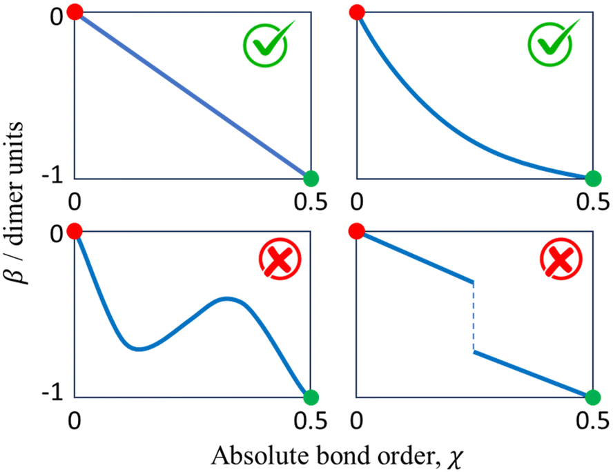 | ||
| Fig. 4 The universal constraints on the bonding function β(χ), χ ∈ [0, 0.5], include two boundary conditions, β(0) = 0 (red circles) and β(0.5) = −1 d.u. (green circles), in addition to the requirements for it to be continuous, monotonic, and well-behaved. | ||
At the other extreme, χ = 1/2, it follows from the definition of the dimer unit that β(0.5) = −1 d.u. (Section 2.3). This limit is indicated by the green dots in each panel in Fig. 4.
In addition to the above boundary conditions, we require the bonding function to be single-valued, monotonic, and well-behaved for χ ∈ [0, 0.5]. Altogether, we expect β(χ) to connect the red (0,0) and green (0.5,−1) points in the (χ, β) plane in a smooth, monotonic fashion. As indicated in Fig. 4, this can be accomplished in a linear or non-linear manner (two sample graphs at the top), but any non-monotonic or discontinuous functions (bottom graphs) must be excluded from consideration. These general features of β(χ), illustrated schematically in Fig. 4, are dictated by universal, monomer-independent constraints.
| β(χ) = −[1 − (1 − 2χ)b2]1/b1 | (7) |
First, given any combination of finite b1, b2 > 0 values, eqn (7) satisfies the β(0) = 0 and β(0.5) = −1 d.u. boundary conditions. The b1 and b2 parameters control how the two limits are connected, but β(χ) is always monotonic, single-valued, and well-behaved. As a limiting case of b1, b2 → ∞, eqn (7) yields the Hückel reference: β = −1 d.u. for any χ > 0.
Nine examples of specific functions defined by eqn (7) are shown in Fig. 5, A–I. Each function shown corresponds to one of the red points in the (b1, b2) parameter space shown in the same figure, top left. Beyond these nine examples, every point in the (b1, b2) space maps onto a unique bonding function. As cases A–I illustrate, b1 controls the β(χ) behaviour near the non-bonding limit (χ = 0), while b2 affects the dimer limit (χ = 0.5). Case E, in particular, with (b1, b2) = (1, 1), corresponds to the linear function β = −2χ shown in panel E on the right.
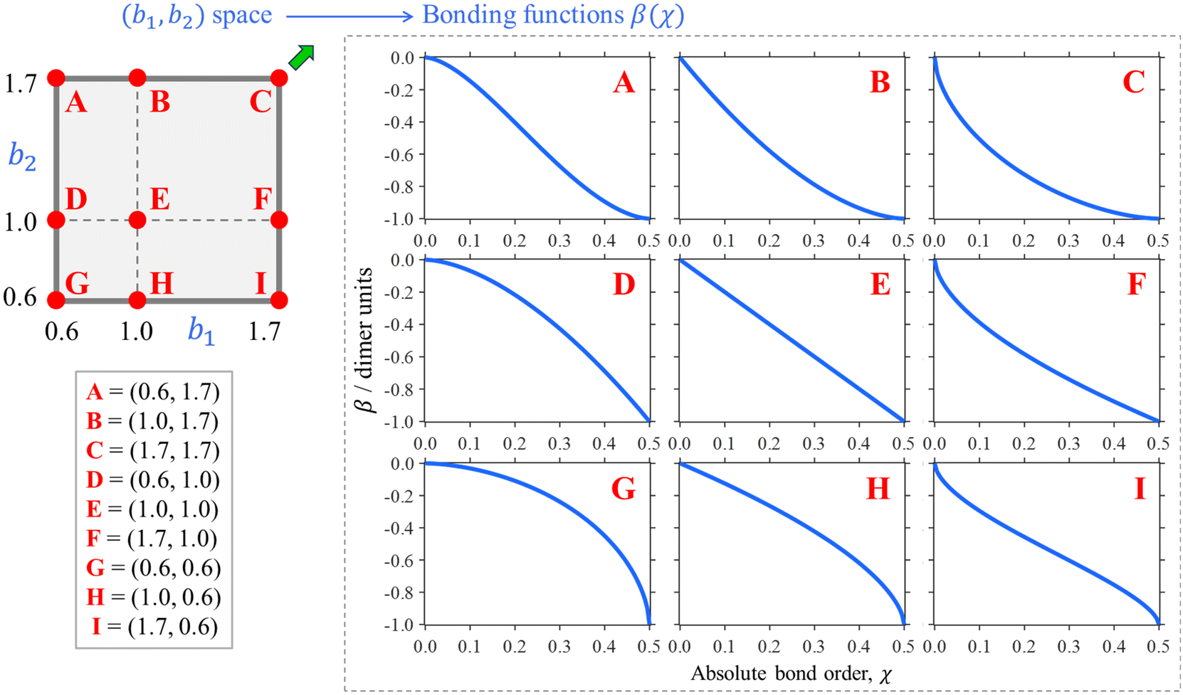 | ||
| Fig. 5 Top left: The (b1, b2) parameter space (“the bonding space”), with boundaries b1, b2 ∈ [0.6, 1.7]. Using eqn (7), each point in this space defines a unique bonding function β(χ). Red circles A–I indicate nine chosen bonding cases, with the corresponding (b1, b2) coordinates indicated below. The corresponding β(χ) are plotted on the right. For reference, of points A–I, C is closest to the Hückel limit (b1, b2 → ∞). The direction towards this limit in the (b1, b2) space is indicated by the green arrow next to point C. | ||
We hypothesise that any given Xn± family can be described by a bonding function represented by a point in the (b1, b2) space. While we do not know a priori what specific (b1, b2) values describe each system, we expect that most common chemical scenario fall well within the b1, b2 ∈ [0.6, 1.7] range shown in Fig. 5. The following analysis will confirm this hypothesis.
We will now examine the mapping of the bonding space to specific core ion structures and compare the results to the known properties of real cluster systems.
3. Initial results
In this section, we test the model using various assumed β(χ) functions. The initial analysis applies to an unspecified Xn± system. Behind such a sweeping approach is the expectation that Xn± clusters have common features attributable to the physics of IM networking rather than the specific chemistry of the monomers. This expectation is rooted partially in the knowledge that in most known cases the excess charge is shared by, at most, three monomers. We show that even the least sophisticated implementation of the model explains this behaviour in a purely coherent regime, without invoking non-covalent interactions or thermal excitations. Section 4 will tune these findings to real chemical systems.3.1. Model convergence
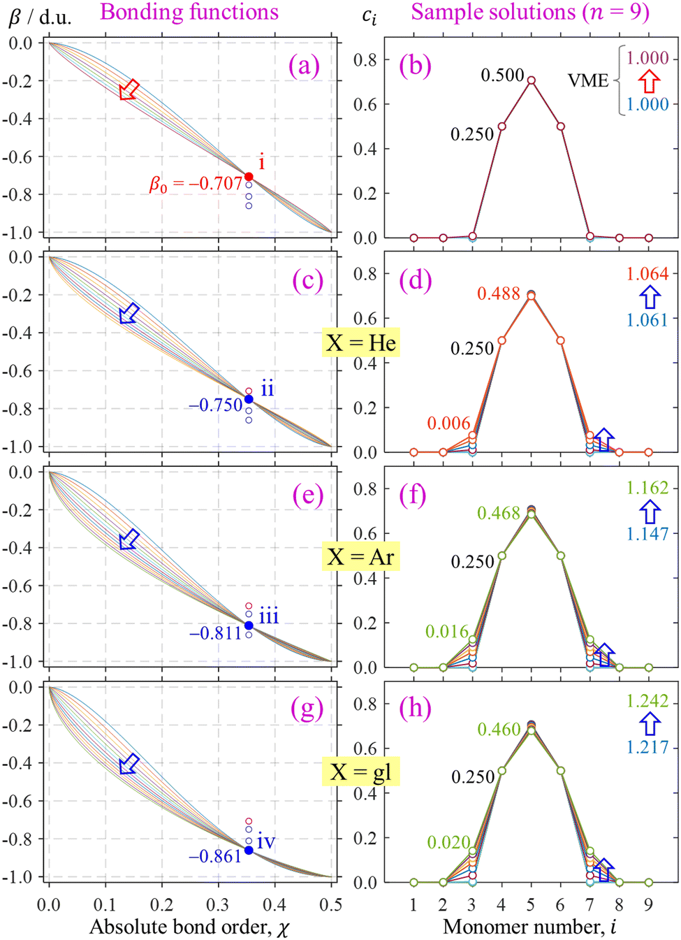
The progress of a typical calculation toward a self-consistent solution is illustrated in Fig. 6 on the example of a nine-membered chain, X9±. There is nothing special about n = 9; this number of monomers is chosen arbitrarily as large enough to illustrate the networking behaviour yet small enough to show details. Similar results can be obtained for shorter or longer chains, and some examples will be given along the way. The Coulomb integrals are set to zero here (in Fig. 6) and throughout (approximation 4.0), while the bond integrals are defined by the bonding function in eqn (7) with b1 = 1.0 and b2 = 1.7. These values correspond to point B in Fig. 5, also shown in the top left of Fig. 6.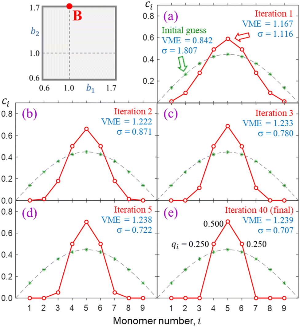 | ||
| Fig. 6 Progress of a typical calculation toward a self-consistent solution on the example of X9±. The calculation was carried out for bonding case B, defined in the top left. The green asterisks in (a)–(e) represent the initial guess, which coincides with the ground state of the particle in a box (dashed grey curves). The red symbols are the IMO coefficients after (a) 1, (b) 2, (c) 3, (d) 5, and (e) 40 iterations. Also shown are the VMEs and charge-sharing sigmas after each iteration. The non-zero partial charges of the monomers are given for the final solution in (e). | ||
The green asterisks in each panel represent the initial {ci} guess used in this calculation. To emphasize the divergence of the model from the Hückel reference, the guess was chosen to coincide with the Hückel solution. That is, it corresponds to the ground state of the particle in a box discretised to nine monomers. For reference, the continuous form of this wave function (half a period of a sin wave) is shown as a dashed grey curve in each panel of Fig. 6. A similar format indicating the initial guess and the Hückel reference is also used in many subsequent figures. The red symbols in Fig. 6 indicate the IMO coefficients after (a) 1, (b) 2, (c) 3, (d) 5, and (e) 40 iterations. This particular calculation required 40 iterations to converge, so the red symbols in (e) represent the final self-consistent solution.
The monomerization energies determined at each iteration viaeqn (3) or, equivalently, eqn (4) are indicated in the figure. The converged solution corresponds to a VME = 1.239 d.u., which is smaller than 1.902 d.u. for the X9± Hückel reference with a constant β = −1 d.u. This distinction is key: our model accounts for geometry relaxation in response to varying bond orders. That results in varying β. Since the equilibrium |β| values are on average smaller than in Hückel's limit, the result is reduced stability.
Most significantly, Fig. 6 shows that the IMO, which is initially delocalised over the entire chain in a particle-in-a-box-like fashion, collapses to just three neighbouring monomers with a 0.25|0.50|0.25 charge distribution. In contrast to the Hückel reference, charge localisation has a stabilising effect in this case because it allows the largest-magnitude bond integrals to receive the most charge. Per eqn (4), this benefits IM bonding. Review the VME progress from the delocalised initial guess to the more localised final solution in Fig. 6 for more detail.
Charge localisation on three monomers can be conveniently expressed in terms of absolute trimer charge  , where qi = |ci|2 and the sum
  is taken over three adjoining monomers with the largest combined charge. For the final solution in Fig. 6(e), Q3 = 1. It implies that the cluster consists of a covalently bonded trimer–ion core, with the other six monomers in a neutral state, not bonded to the core or to each other: X3±·X6. We will refer to trimer ions with Q3 = 1 as “pure” trimers or trimers of 100% purity. We shall see that pure trimers are a common phenomenon in the coupled-monomers model, not limited to X9± or the exact numerical assumptions used to generate Fig. 6.
Charge sharing can be quantified for any system (not limited to trimers) using the standard deviation (σ) of the charge distribution. The distribution is defined by Pi = |ci|2 = ρi,i, and the standard deviation of i is calculated as  . We will refer to it as charge-sharing σ. Its values after each iteration are included in Fig. 6. For comparison, the X9± Hückel reference and the initial guess in Fig. 6 are described by σ = 1.807, while for the final solution in Fig. 6(d)
 .
.
3.2. Local solutions
Final solutions generally depend on the initial guess and this is particularly important for longer chains. For illustration, Fig. 7 presents three distinct solutions (a)-(c) for X25± using the bonding function defined by point F in the (b1, b2) space. The solutions obtained from distinct sets of initial {ci} coefficients differ in their placement along the chain, but their key properties are identical, including the VMEs and charge distributions within the core ion. In each case, 96.8% of the charge is localised on three core monomers (Q3 = 0.968), and only the specific monomer trio capturing the charge differs. The reduced trimer purity sets case F in Fig. 7 apart from case B in Fig. 6(e) (Q3 = 1). The reduction is due to a faster increase in |β| near χ = 0 evident in Fig. 5, F vs. B. The faster increase in F is in turn due to a larger b1.The degenerate solutions in Fig. 7 are local in the n-dimensional vector space |ϕ〉 and localised to a small number of monomers. Since monomers with zero ci coefficients do not contribute to covalent bonding, we can add or remove any such inactive monomers without affecting the core-anion properties. This means changing the dimensionality of the |ϕ〉 vector space outside the active subspace describing the core. Physically, it implies adding or removing spectator monomers that do not interact with the bulk of the cluster. For example, the core properties of the solutions in Fig. 7 (VME, σ, and Q3) would not be affected if the chain were expanded or shrunk to any n ≥ 5.
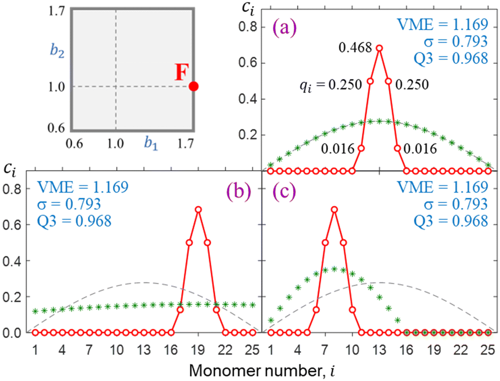 | ||
| Fig. 7 (a)–(c) Distinct but degenerate X25± solutions for bonding case F. In each case, the initial {ci} guess is indicated by green asterisks. | ||
3.3. Ground-state structures
The above realisation can be used to facilitate a global search for lowest-energy self-consistent solutions. To ensure that a given solution describes a relaxed ground-state structure we must generally perform an exhaustive search in the |ϕ〉 vector space. That requires calculations starting from a multitude of initial states to sample various regions of the n-dimensional space. This is impractical for more than a few monomers. Instead, we take advantage of the fact that as long as edge effects are avoided, the converged solutions always contain symmetric core ions: a monomer, dimer, trimer, etc. Meanwhile, any number of spectator monomers with ci = 0 can be added or removed at will for computational convenience without affecting the core solution.Hence, for every point sampled in the (b1, b2) space we carried out two calculations: one for an even and one for an odd number of monomers. For computational expediency, while still avoiding the edge effects, we chose n = 8 and 9. In each case, the Hückel reference was used as the initial guess. All resulting {ci} solutions were symmetric with respect to the middle of the chain (i = 5 for n = 9 and halfway between i = 4 and 5 for n = 8), constraining the ionic core to an odd or even number of monomers, respectively. We then compared the odd- and even-n solutions and designated the core ion within the more stable one as the equilibrium core structure for that bonding function.
This approach is illustrated in Fig. 8 for bonding cases H, E, B, and C (all defined in Fig. 5). In case H, the even-numbered core structure in Fig. 8 (a pure dimer with a VME = 1 d.u.) is more stable than an odd-numbered one (a pure trimer, VME = 0.728 d.u.). Thus, we expect any system with a bonding function represented by point H (or its vicinity) in the (b1, b2) space to have a dimer-ion core.
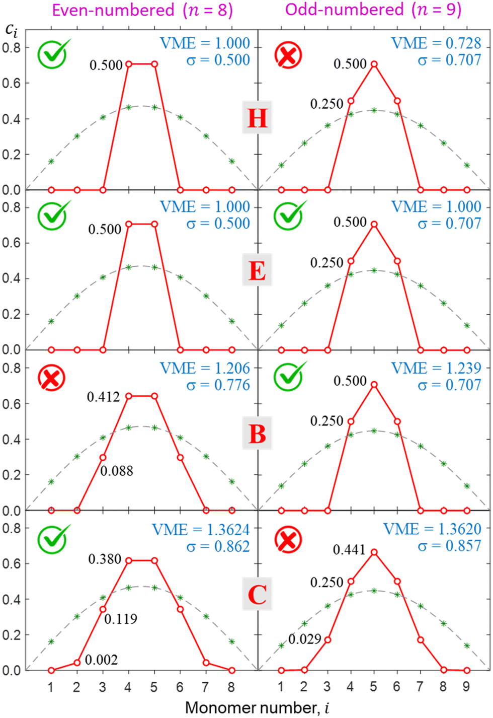 | ||
| Fig. 8 Top to bottom: the final solutions for bonding cases H, E, B, and C from Fig. 5. Left and right columns correspond to the even- (n = 8) and odd- (n = 9) numbered Xn± chains. Each calculation used the respective Hückel reference as the initial guess and was thus constrained to even- or odd-numbered core type. Check and cross marks indicate the more and less stable structures, respectively, for each bonding case. In case E, the even- and odd-numbered structures are degenerate (both have checkmarks). | ||
Case E represent a transition between the dimer and trimer phases. With (b1, b2) = (1, 1), the bonding function in eqn (7) simplifies to β = −2χ. The pure-trimer solution  includes two IM bonds with
  and
and  d.u. each. Each bond's energy is then, per eqn (4), −2βχ = 1/2 d.u., for a combined VME = 1 d.u. exactly, which is degenerate with the dimer structure.
In case B, trimer-based structures are most favourable. The even-numbered solution on the left in Fig. 8 in this case is no longer a pure dimer; it resembles a tetramer instead. Each of the two middle monomers within the tetramer core has an absolute charge of q2,3 = 0.412 with q1,4 = 0.088 localised on the terminal species. However, this tetramer-based structure is less stable than its trimer-based counterpart on the right.
The situation is reversed in case C, where the even-numbered core ion is more stable than its odd-numbered counterpart. We should recall that of all bonding cases A–I defined in Fig. 5, case C is closest to the Hückel limit of β = −1 = const. It is not surprising, therefore, that the solutions obtained in this case have the widest charge distributions compared to any other case examined thus far (note the σ values in Fig. 8). The most stable core structure in case C is essentially a tetramer with a 0.119|0.380|0.380|0.119 charge distribution, but the solution also reveals a minor (0.2%) charge spillover to each of the monomers immediately adjacent to the tetramer core. An even greater spillage from the core is present in the nearly degenerate but slightly less stable odd-numbered solution for case C, where each of the two monomers adjacent to the trimer core (Q3 = 0.94) captures nearly 3% of the charge. If we were to continue the journey along the GC diagonal in the bonding space (Fig. 5) beyond case C, the solutions would get progressively broader, approaching the Hückel case (dashed grey curves in Fig. 6–8) in the limit of b1, b2 → ∞.
3.4. Dimers, trimers, and beyond
Fig. 9 presents a coarse overview of the bonding space from Fig. 5, illustrating the effect of varying the bonding function on the core-ion properties. Each panel A–I in Fig. 9 corresponds to the respective bonding case in Fig. 5. Unlike Fig. 8, all solutions in Fig. 9 were obtained for an odd-membered chain X9±. However, the initial guess was varied in each case to obtain both odd and even-numbered core structures and only the lowest-energy solutions are presented in the figure. In case E, the dimer and trimer-based solutions are exactly degenerate, with VME = 1 d.u. each, and only the trimer-based is shown.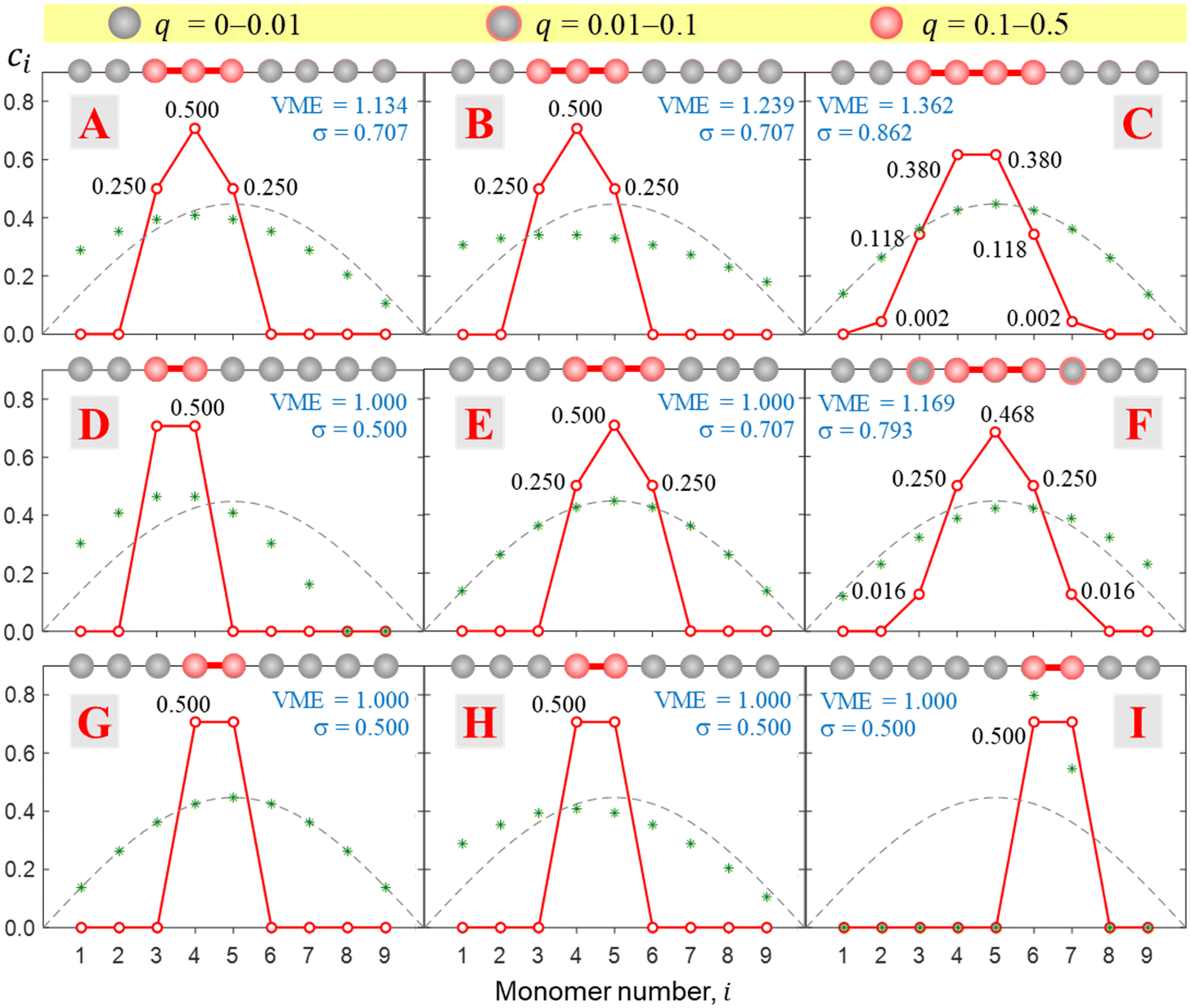 | ||
| Fig. 9 Most stable final solutions identified for bonding cases A–I. All solutions were obtained for an odd-membered chain X9± but the initial guess was varied to identify both odd and even-numbered core structures, and only the most stable solutions are presented in figure. In case E, the dimer and trimer-based solutions are exactly degenerate, with VME = 1 d.u. each, but only the trimer-based is shown. | ||
While Fig. 9 displays sample solutions on a 3 × 3 grid in the (b1, b2) bonding space, a more refined picture is presented in Fig. 10. Here, following the methodology from Section 3.3, we analysed the X8± and X9± solutions on a 201 × 201-point (b1, b2) grid. The resulting values of VME(b1,b2) and σ(b1,b2) for the more stable structures are presented in (a) and (b), respectively, as two-dimensional contour plots. In (c), the σ(b1,b2) data from (b) are plotted again as a 3-D surface. Since inactive monomers can be added or removed at will (Section 3.3), these results are valid for any-size Xn± chains, as long as edge effects are avoided.
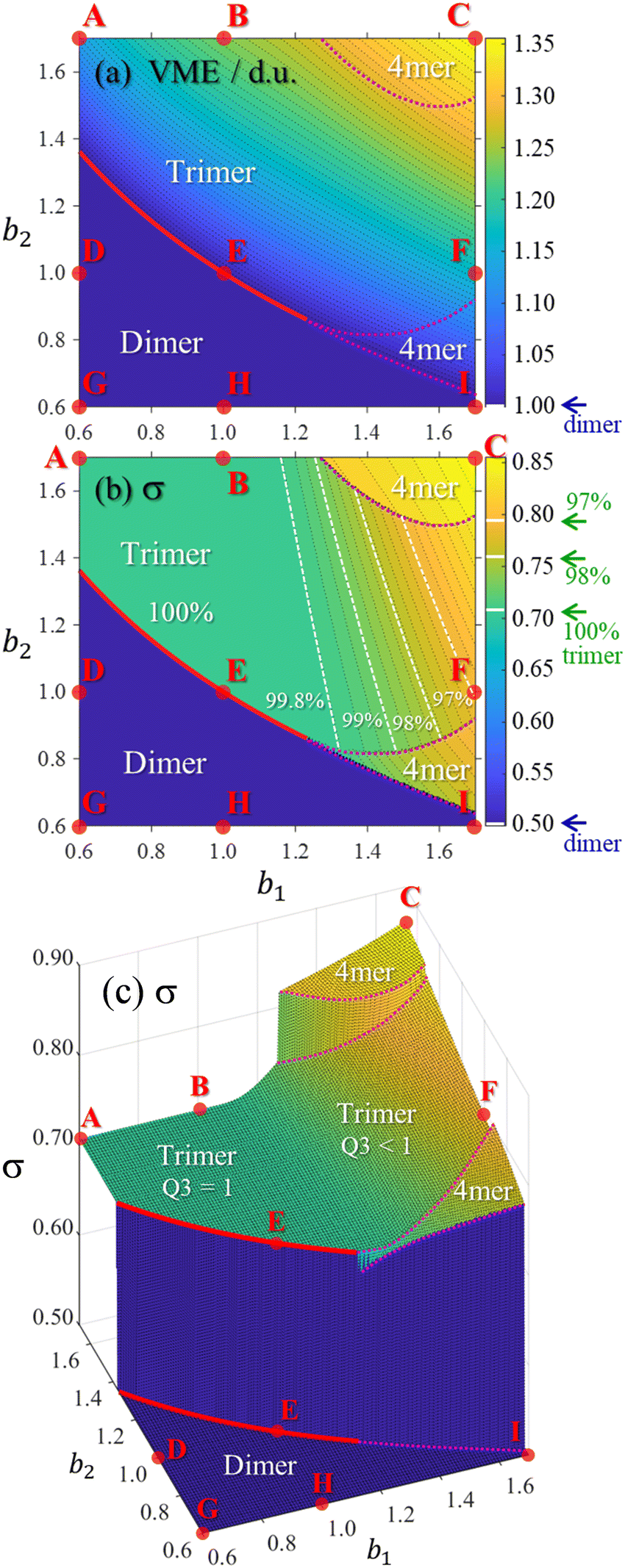 | ||
| Fig. 10 The (a) VME and (b) and (c) charge-sharing σ plots calculated on a 201 × 201-point grid in the bonding space (b1, b2) ∈ [0.6, 1.7]. The same σ(b1, b2) dataset is shown in (b) and (c) using two different formats. All data represent the most stable core structures identified for each bonding case and the resulting dimer, trimer, and tetramer (“4mer”) regions are labelled in each plot. Points A–I indicate the bonding cases defined in Fig. 5. The red solid curves indicate the boundary between the dimer and trimer regions. The top and bottom red curves in (c) are the same boundary, plotted twice, at the dimer and trimer σ levels. The dotted magenta curves represent similar dimer–tetramer and trimer–tetramer boundaries. The white dashed lines in (b) correspond to (left to right) 99.8%, 99%, 98%, and 97% trimer purity. | ||
Fig. 10 shows that increasing b1 and b2 generally increases the cluster stability (larger VME) and leads to more delocalised charge distributions (larger σ). Both trends are intuitive because as b1, b2 → ∞ the model approaches the particle-in-a-box-like Hückel limit. While the energetic trend in (a) is described by a smooth and continuous VME(b1,b2) dependence, the σ(b1,b2) data show sharp discontinuous transitions reflecting changes in the ionic core structure.
Considering the charge distributions in detail, σ = 0.5 corresponds to a pure dimer-ion cluster core with partial charges qi = 0.5|0.5. A pure trimer (Q3 = 1, qi = 0.25|0.50|0.25) has a 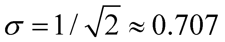 . Several correlations between Q3 and σ are indicated in Fig. 10(b) next to the σ colour bar. Using the discontinuities in σ and analysing the {ci} solutions, the (b1,b2) space can be divided into the dimer, trimer, and tetramer (4mer) regions shown in Fig. 10(a)–(c). The trimer region can be additionally subdivided into the pure (Q3 = 1 exactly) and impure (Q3 < 1) areas, labelled in (c). Their strict boundary corresponds to the BE line, but even to the right of it the initial increase in σ and the corresponding decrease in Q3 are very slow at first. Fig. 10(b) shows white dashed lines corresponding to Q3 = 0.998, 0.99, 0.98, and 0.97, indicated as percentages to the left of the lines.
While the variation of trimer purity is gradual and not associated with discontinuities in the charge distribution, the dimer–trimer, trimer–tetramer, and dimer–tetramer transitions are defined by sharp boundaries with abrupt discontinuities in charge sharing. The most drastic change, from σ = 0.5 to 0.707, occurs at the dimer–trimer interface, i.e., the solid red curve in Fig. 10. This curve terminates at a point where the dimer–trimer boundary bifurcates into the dimer–tetramer and trimer–tetramer borders.
Overall, the trimer region encompasses a significant area of the (b1,b2) space. Importantly, in the future we plan to show that the bonding properties of many known Xn± families fall close to the BH line within this space (Fig. 5 and 10). The preference for either dimer or trimer core ions is largely determined by whether the bonding function for a specific system corresponds to a point below or above point E on this line, as is clear from Fig. 10(b) and (c). For example, the existence of the X = He, Ar, gl, and ba trimer ions9,50,55,56,66–68 suggests that their bonding properties fall above point E in the (b1, b2) space, corresponding to b2 > 1.
4. Data-driven modelling
In this section, we use available data for several Xn± systems to determine which of the bonding functions defined in Section 3 are closest to chemical reality.4.1. General model training
Section 2.4 defined two universal constraints on the bonding function: the boundary conditions at the non-bonding and dimer limits, β(0) = 0 and β(0.5) = −1. These boundary conditions are independent of the nature of the monomers and therefore help little in identifying the unique bonding properties of specific systems. This is illustrated in Fig. 11, where a myriad of allowed bonding functions, 144 in total, are plotted in part (b).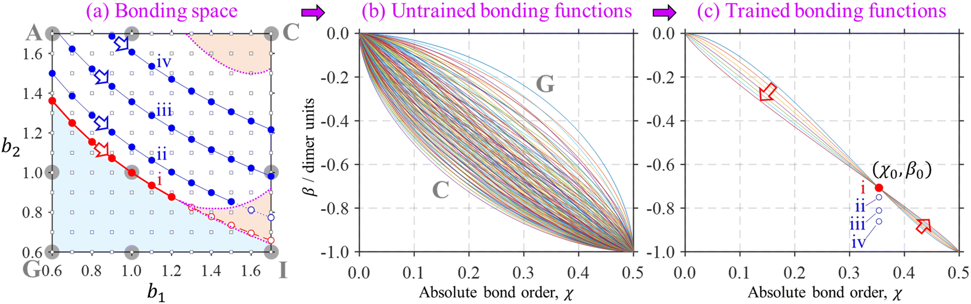 | ||
Fig. 11 An illustration of the bonding function training process. (a) A snapshot of the bonding space including original 3 × 3 reference points A–I from Fig. 5, shown here by large grey circles. The dimer region of the bonding space is shaded in blue, tetramer-orange, the trimer region is unshaded. The corresponding region boundaries are indicated similarly to Fig. 10. These details are overlaid with a finer 12 × 12 grid of the (b1, b2) parameter values, shown by small black squares. (b) 144 (= 12 × 12) bonding functions defined by eqn (7) for the 12 × 12 grid shown in (a). (c) Seven (instead of 144) distinct β(χ) functions defined on a similar (b1, b2) grid but subject to the dimer/trimer degeneracy constraint, 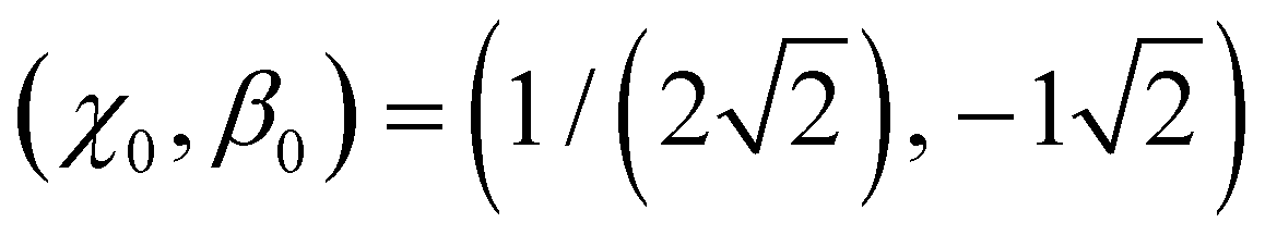 , which is marked ‘i’. Each of the bonding functions corresponds to one of the solid red symbols along the dimer–trimer boundary (curve ‘i’) in (a). Training points ii–iv, with β0 = −0.750, −0.811, and −0.861 d.u., (X = He, Ar, gl) similarly correspond to respective curves in (a). See the text for further details. , which is marked ‘i’. Each of the bonding functions corresponds to one of the solid red symbols along the dimer–trimer boundary (curve ‘i’) in (a). Training points ii–iv, with β0 = −0.750, −0.811, and −0.861 d.u., (X = He, Ar, gl) similarly correspond to respective curves in (a). See the text for further details. | ||
This part of the figure is messy by design and not intended to be analysed in detail. Although all functions shown satisfy the boundary conditions, altogether they represent an overwhelming range of possible bonding scenarios, most of which are of little use for real chemistry. This changes with the introduction of just one additional constraint. In general terms, we define it as β(χ0) = β0, requiring the bond integrals to have a specific value β0 ∈ (−1, 0) for a chosen bond order χ0 ∈ (0, 0.5). We will refer to (χ0, β0) as the training point and will shortly show how it relates to specific chemical properties.
Requiring the bonding function to pass through a specific training point drastically restricts the space of acceptable β(χ), as evident in Fig. 11(c). In detail, the bonding functions in Fig. 11(b) are all defined by eqn (7) on a 12 × 12 grid in the (b1, b2) parameter space. The grid is indicated by small black squares in Fig. 11(a). It represents an expansion of the original 3 × 3 grid A–I from Fig. 5, reproduced in Fig. 11(a) for reference (large grey circles). Among the myriad of curves in Fig. 11(b), the lowest and the topmost represent cases C and G, respectively.
Now we consider an arbitrary (χ0, β0) constraint. Rearranging eqn (7),
| b2 = log(1−2χ0)[1 − (−β0)b1] | (8) |
4.2. The dimer–trimer boundary
The dimer–trimer boundary is defined by an X2± and X3± degeneracy. Since the dimer bond energy is 1 d.u. by definition, the degeneracy requires each bond in the trimer to be exactly 1/2 d.u. On the other hand, the energy of a bond is given, per eqn (4), by −2χβ. From the normalised IMO coefficients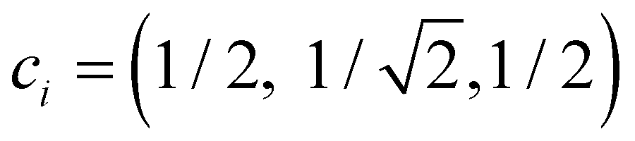 , the order of each bond in linear X3± is
  . It follows that the dimer–trimer degeneracy is defined by
  and the dimer–trimer transition in the bonding space occurs when
 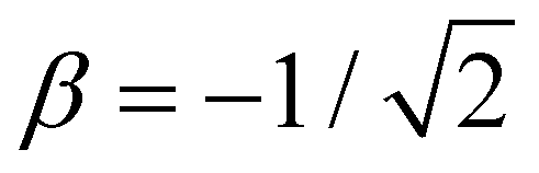 d.u. for
 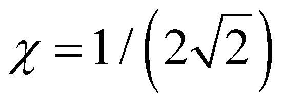 .
.
With  as the training point, eqn (8) yields an analytic relationship between b1 and b2, which defines the dimer–trimer boundary in the bonding space. It is shown by red solid curves in Fig. 10(a)–(c) and 11(a), marked ‘i’ in 11(a). The b2 = b2(b1) boundary curve can be calculated for the entire range of b1, but for b1 ≳ 1.2 it bifurcates into dimer–tetramer and trimer–tetramer transitions, shown as dotted magenta curves in each Fig. 10(a)–(c) and 11(a). The dimer–trimer interface then loses significance, passing through a tetramer region where both dimers and trimers are metastable structures. The continuation of the dimer–trimer curve in the tetramer region is nonetheless shown in Fig. 11(a) (red dashed curve with red open symbols). For clarity, the tetramer regions are shaded in orange, the dimer region is in light blue, while the trimer region is unshaded.
Each point on curve ‘i’ in Fig. 11(a) defines a unique function β(χ) passing through the above training point and satisfying the dimer–trimer degeneracy. The training point itself is represented by a red symbol in Fig. 11(c). The trained β(χ) curves in the same figure [only seven total, compared to 144 untrained curves in (b)], represent the filled red (b1, b2) symbols on the dimer–trimer boundary in (a). The red block arrows in Fig. 11(a) and (c) indicate the direction of β(χ) variation along this boundary. Moving to the right along curve ‘i’ in (a) causes the β(χ) curves in (c) to change in the downward direction to the left of the training point and in the upward direction to the right of (χ0, β0).
The trained bonding curves from Fig. 11(a) are reproduced in Fig. 12(a) next to a sample of odd-numbered (X9±) IMO solutions in Fig. 12(b). There are 7 overlapping solutions shown, one for each of the solid-red (b1, b2) points along curve ‘i’ in Fig. 11(a). They are indistinguishable from each other, each possessing a pure-trimer core (Q3 = 1), with a VME = 1.000 d.u. (degenerate with dimer-core structures).
 | ||
| Fig. 12 Left column: Trained bonding curves satisfying the indicated (χ0, β0) constraints i–iv. Curves in (a) for training point ‘i’ are reproduced from Fig. 11(c). Training points ii–iv correspond to Xn±, X = He, Ar, and gl, respectively. Right column: Samples of IMO solutions obtained with the respective bonding functions shown on the left. | ||
4.3. Model training for specific systems
Many specific cluster families exhibit a propensity for trimer–ion cores. For trimer-based structures, not all parts of the bonding function are equally important to the model performance, since only a small part of β(χ) in the vicinity of plays a defining role in the final solutions.
This may seem like an invitation to replace β(χ), χ ∈ [0, 0.5], with a single value, β0 = β(χ0), but that would be a mistake. A model limited to a single bond order is not able to access other Xn± configurations, including the dimer- or tetramer-based structures. The trimer core then ceases being a prediction and becomes the only achievable outcome. To claim that a particular configuration is preferable to others, the model must sample a broad range of configuration space, which requires χ to vary. It is nonetheless possible to emphasise the region around χ = χ0 while treating other parts of β(χ) in a less precise fashion.
This is done by training the model to reproduce the known monomerization energies of X3±, VME(3), using a single (χ0, β0) training point for each cluster type. The important role of the trimer ions suggests that VME(3) is both a convenient and critical measure for calibrating and assessing the model performance. The mathematical essence of the training process is a reduction of the space of all bonding functions defined by eqn (7) to a subspace that accurately describes the bonding in a specific Xn± system. This objective is achieved using the (χ0, β0) training data and eqn (7) in a manner similar to the analysis of the dimer–trimer boundary in Section 4.2.
Per eqn (4), for linear X3±, VME(3) = −2 × 2χ0β0, where 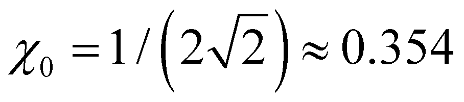 is the trimer bond order from Section 4.2. This yields β0 = −VME(3)/(4χ0) for the trimer bond integral. The known VME(3) values in Table 1 therefore allow us to determine the (χ0, β0) training points for each of the specific systems considered. They correspond to β0 = −0.750, −0.811, and −0.861 d.u. for X = He, Ar, and gl. In the same way, β0 = −1 d.u. for the Hückel reference and β0 = −1.10 d.u. for X = ba (vide infra).
The training points for X = He, Ar, and gl are indicated by symbols ‘ii’, ‘iii’, and ‘iv’ in Fig. 11(c), under the training point for the dimer–trimer boundary marked ‘i’. Section 4.2 discussed that training point ‘i’ reduced the (b1, b2) bonding space to a one-dimensional subspace ‘i’ shown by a red curve in Fig. 11(a). Similarly, training points ‘ii’, ‘iii’, and ‘iv’ in Fig. 11(c) reduce the permissible bonding space to the respectively marked blue curves in Fig. 11(a). Similar to ‘i’ (Section 4.2), the rightmost (dotted) part of curve ‘ii’ is excluded from consideration, because trimer-based training should not be used in the tetramer region.
Training points ii–iv are reproduced in Fig. 12(c), (e) and (g), respectively, which also show the bonding functions defined by each of the filled symbols on the respective curves in Fig. 11(a). Like the analysis of curve ‘i’ bonding functions in Section 4.2, the block arrows in Fig. 12(c), (e) and (d) indicate the direction of β(χ) variation along the respective curves in Fig. 11(a). The corresponding solutions (specifically, for X9±) are shown in Fig. 12 on the right, one solution for each trained bonding function.
All solutions for X = He, Ar, and gl in Fig. 12 are consistent with the predictions of high-level ab initio and density-functional theory.9,50,55,56,66–68 Importantly, they have very similar properties. These similarities are present both among solutions for each specific system and across the systems discussed. There are certainly differences in the VMEs imposed by the training points. The slight increase in VME across the solutions for the same system (e.g., from 1.061 d.u. to 1.064 d.u. for X = He) is due to the minor charge spillage off the trimer core. Accordingly, there are slight variations in trimer–core purity (Q3) among solutions for the same system. Like VME, timer purity is dependent on specific bonding functions. It decreases somewhat with increasing b1, as seen in Fig. 10(b) and (c). Naturally, off-the-trimer charge spillage and VME variation are only possible in chains with n > 3. In an isolated trimer, Q3 would always be strictly 1 with a 0.25|0.50|0.25 charge distribution, and VME(3) would be constant for any bonding function satisfying a specific training point.
These small differences aside, the various solutions for all systems considered correspond to, essentially, trimer-based clusters, with Q3 ranging from 100% to 98.8% for X = He, 100% to 96.8% for X = Ar, and 100% to 96.0% for X = gl. To make more definitive predictions about core purity, a more in-depth analysis of the bonding properties in the small χ region is required, leading to additional training constraints.
4.4. Limitations and future directions
Two of the model limitations go beyond the approximate nature of the described formalism. The first has to do with the ban− clusters, the second with charge distributions among core monomers.The VME of the trimer anion of biacetyl exceeds that of the dimer by 55.2%,9 corresponding to a VME(3) = 1.552 d.u. (Table 1). From the coupled-monomers perspective, this is an abnormally large value unlike the other examples discussed, because it exceeds the corresponding property of the Hückel reference,  8,25 As determined in Section 4.3, a VME(3) of 1.552 d.u. requires the trimer bond integral to equal −1.10 d.u., with the magnitude exceeding that of the equilibrium bond integral in the dimer (−1 d.u. exactly). This contradicts one of our assumptions requiring the β(χ) bonding function to be monotonic between the β(0) = 0 and β(0.5) = −1 limits (Fig. 4).
This result becomes less puzzling if instead of interpreting it as VME(3) for X = ba being too large, we reframe it as VME(2) being too small. The reduced bond strength in relaxed ba2− can be attributed in part to a steric obstruction of the methyl groups preventing the two ba moieties from coming close enough to realise the full bonding power of the shared electron. In the trimer, the IM distance is larger, and the methyl steric effects are less significant. This alone cannot explain the abnormal stability of ba3−: at most, it would cause VME(3) for X = ba to approach the Hückel limit of 1.414 d.u., not 1.552 d.u. However, there are additional factors that have not been considered by the present formulation of the model. One of them, the variable Coulomb integrals (approximation 4.1 in Section 2.1), we plan to address in the future.
Another limitation is also related to variable Coulomb integrals, among other factors. It concerns the charge distributions among core monomers. High-level ab initio data show that the charge distribution in He3+ is somewhat broader than 0.25|0.50|0.25, while the opposite is true for Ar3+.56,68 Our present model treats both X = He and X = Ar exactly the same, aside from the different energetics which do not affect the charge distributions. Therefore, in its present form, the model is incapable of predicting the different behaviours of the He- and Ar-based clusters regarding the core charges.
We will conclude by pointing out two factors that affect the partial charges within the cluster core (and its stability): the remote interactions between non-adjacent monomers and the variable Coulomb integrals. Our future work will incorporate both into the coupled-monomers formalism to demonstrate that it is the Coulomb integrals, not the remote forces, that control the divergent charge distributions in various cluster families.
Furthermore, in the present work we have made no significant distinction between anion and cations, or between electrons and holes. This is an important omission because electrons do behave differently from holes with respect to some aspects of chemical bonding. It will be shown that the very qualitative character of remote IM interactions depends not only on the type of the bonding agent (electrons or holes) but also the symmetry of the MMOs defining the IMO system. In some qualitative respects, the gln− and ban− cluster anions are more like Hen+ cluster cations than Hen+ are like Arn+.
Finally, in this work we considered the behaviour of only one electron (hole). Since radical species tend to react further, the one-electron picture will break down in some applications. It is therefore a strength of the coupled-monomers model (like the original Hückel theory) that it is not inherently limited to one-particle systems. Here, we started from the extreme of a single bonding agent responsible for the entire covalent network, but the fundamental model can be developed further.
5. Summary
We have described a density-matrix adaptation of the Hückel MO theory to weak covalent networks and used the resulting model to examine the interactions of electrons (holes) with ensembles of identical closed-shell monomers.Like the Hückel method, the coupled-monomers model provides chemically accurate qualitative and semi-quantitative answers that emphasise physical insight over the precision and complexity of higher-level ab initio theory. The main distinguishing feature of the model is the use of variable bond and (in future work) Coulomb integrals defined by the density matrix. The performance of the model can be significantly improved by training it to experimental or ab initio data.
Quantitative details notwithstanding, the model makes a bold prediction: within a wide parameter range, Xn± clusters tend to have core ions comprised of two or three monomers. The validity of this prediction is confirmed by many known cluster families. The preponderance of dimer and trimer ions is due to the more effective conversion of the bonding power of one electron (hole) into bond energy. This occurs via the formation of one or two equivalent bonds with large bond orders and, therefore, large-magnitude bond integrals.
Various alternative competing mechanisms that favour either charge sharing or charge localisation help set this prediction in context. While covalent bonding is the main driving force for coherent charge sharing, several well-known factors may instead favour more localised charge distributions and, therefore, smaller cluster cores. They include: (i) the non-covalent interactions favouring smaller ions; (ii) the entropic contribution to free energy favouring less-ordered solvated structures; and (iii) the loss of electronic coherence due to vibronic and other couplings.
The coupled-monomers model is formulated here in a strictly coherent and covalent regime, without any non-covalent forces or thermal excitations. And yet, even in the absence of factors (i)–(iii), it still predicts rather localised charge distributions. It follows that although charge localisation may benefit from these complex mechanisms, it does not have to rely on any of them. It is an intrinsic feature of a coherent, purely covalent weakly bonded network, arising from geometry relaxation and correlation between bond orders and the relaxed bond integrals.
Conflicts of interest
There are no conflicts to declare.Acknowledgements
This work is supported by the U.S. National Science Foundation (grant CHE-2153986).Notes and references
- C. A. Kraus, J. Am. Chem. Soc., 1908, 30, 1323 CrossRef CAS.
- K. D. Jordan and F. Wang, Annu. Rev. Phys. Chem., 2003, 54, 367 CrossRef CAS PubMed.
- N. I. Hammer, R. J. Hinde, R. N. Compton, K. Diri, K. D. Jordan, D. Radisic, S. T. Stokes and K. H. Bowen, J. Chem. Phys., 2004, 120, 685 CrossRef CAS PubMed.
- H.-J. Schneider, Angew. Chem., Int. Ed., 2009, 48, 3924 CrossRef CAS PubMed.
- A. J. Stone, The Theory of Intermolecular Forces, Oxford University Press, Oxford, 2013 Search PubMed.
- V. K. Voora, A. Kairalapova, T. Sommerfeld and K. D. Jordan, J. Chem. Phys., 2017, 147, 214114 CrossRef PubMed.
- C. Mackie, A. Zech and M. Head-Gordon, J. Phys. Chem. A, 2021, 125, 7750 CrossRef CAS PubMed.
- A. Sanov, Int. Rev. Phys. Chem., 2021, 40, 495 Search PubMed.
- Y. Dauletyarov and A. Sanov, Phys. Chem. Chem. Phys., 2021, 23, 11596 RSC.
- C. C. Jarrold, ACS Phys. Chem. Au, 2023, 3, 17 CrossRef CAS PubMed.
- U. Schindewolf, Angew. Chem., Int. Ed. Engl., 1978, 17, 887 CrossRef.
- F. Arnold, Nature, 1981, 294, 732 CrossRef CAS.
- G. H. Lee, S. T. Arnold, J. G. Eaton, H. W. Sarkas, K. H. Bowen, C. Ludewigt and H. Haberland, Z. Phys. D: At., Mol. Clusters, 1991, 20, 9 CrossRef CAS.
- C. Desfrancois, H. Abdoulcarime, N. Khelifa and J. P. Schermann, J. Chim. Phys. Phys.-Chim. Biol., 1995, 92, 409 CrossRef CAS.
- P. Ayotte, G. H. Weddle, C. G. Bailey, M. A. Johnson, F. Vila and K. D. Jordan, J. Chem. Phys., 1999, 110, 6268 CrossRef CAS.
- M. Gutowski, C. S. Hall, L. Adamowicz, J. H. Hendricks, H. L. de Clercq, S. A. Lyapustina, J. M. Nilles, S. J. Xu and K. H. Bowen, Phys. Rev. Lett., 2002, 88, 143001 CrossRef CAS PubMed.
- T. Sommerfeld and K. D. Jordan, J. Am. Chem. Soc., 2006, 128, 5828 CrossRef CAS PubMed.
- K. R. Siefermann and B. Abel, Angew. Chem., Int. Ed., 2011, 50, 5264 CrossRef CAS PubMed.
- R. M. Young and D. M. Neumark, Chem. Rev., 2012, 112, 5553 CrossRef CAS PubMed.
- E. Hückel, Z. Phys., 1931, 70, 204 CrossRef.
- E. Hückel, Z. Phys., 1931, 72, 310 CrossRef.
- E. Hückel, Z. Phys., 1932, 76, 628 CrossRef.
- E. Hückel, Z. Phys., 1933, 83, 632 CrossRef.
- N. C. Baird and M. A. Whitehead, Can. J. Chem., 1966, 44, 1933 CrossRef CAS.
- I. N. Levine, Quantum Chemistry, Prentice-Hall, Upper Saddle River, NJ, 2000 Search PubMed.
- L. Pauling, J. Am. Chem. Soc., 1947, 69, 542 CrossRef CAS.
- P. T. Lang, Found. Chem., 2023 DOI:10.1007/s10698-023-09486-7.
- B. Zulueta, S. V. Tulyani, P. R. Westmoreland, M. J. Frisch, E. J. Petersson, G. A. Petersson and J. A. Keith, J. Chem. Theory Comput., 2022, 18, 4774 CrossRef CAS PubMed.
- C. D. Clark, Nature, 1939, 143, 800 CrossRef CAS.
- J. L. Kavanau, J. Chem. Phys., 1947, 15, 77 CrossRef CAS.
- R. D. Brown, Aust. J. Sci. Res., Ser. A, 1949, 2, 564 Search PubMed.
- G. Nebbia, J. Chem. Phys., 1950, 18, 1116 CrossRef CAS.
- L. S. Bartell, J. Phys. Chem., 1963, 67, 1865 CrossRef CAS.
- W. H. Weinberg, J. Vac. Sci. Technol., 1973, 10, 89 CrossRef CAS.
- B. A. Hess and L. J. Schaad, Z. Phys. Chem. (Leipzig), 1979, 260, 183 CrossRef.
- V. Velenik, T. Zivkovic and N. Trinajstic, Rev. Roum. Chim., 1984, 29, 737 CAS.
- P. Politzer and S. Ranganathan, Chem. Phys. Lett., 1986, 124, 527 CrossRef CAS.
- I. Mayer, M. Knapp-Mohammady and S. Suhai, Chem. Phys. Lett., 2004, 389, 34 CrossRef CAS.
- C. Oberdorfer and W. Windl, Acta Mater., 2019, 179, 406 CrossRef CAS.
- J. V. Ortiz, Adv. Quantum Chem., 1999, 35, 33 CrossRef CAS.
- A. I. Krylov, J. Chem. Phys., 2020, 153, 080901 CrossRef CAS PubMed.
- D. Licari, S. Rampino and V. Barone, Lect. Notes Comput. Sci., 2019, 11624, 388 Search PubMed.
- S. H. Fleischman and K. D. Jordan, J. Phys. Chem., 1987, 91, 1300 CrossRef CAS.
- M. J. DeLuca, B. Niu and M. A. Johnson, J. Chem. Phys., 1988, 88, 5857 CrossRef CAS.
- T. Tsukuda, M. A. Johnson and T. Nagata, Chem. Phys. Lett., 1997, 268, 429 CrossRef CAS.
- M. Saeki, T. Tsukuda and T. Nagata, Chem. Phys. Lett., 2001, 348, 461 CrossRef CAS.
- M. Saeki, T. Tsukuda and T. Nagata, Chem. Phys. Lett., 2001, 340, 376 CrossRef CAS.
- R. Mabbs, E. Surber, L. Velarde and A. Sanov, J. Chem. Phys., 2004, 120, 5148 CrossRef CAS PubMed.
- Y. Dauletyarov, A. A. Wallace, C. C. Blackstone and A. Sanov, J. Phys. Chem. A, 2019, 123, 4158 CrossRef CAS PubMed.
- F. X. Gadea and I. Paidarová, Chem. Phys., 1996, 209, 281 CrossRef CAS.
- F. Y. Naumkin and D. J. Wales, Mol. Phys., 1998, 93, 633 CAS.
- W. R. Wadt, J. Chem. Phys., 1980, 73, 3915 CrossRef CAS.
- T. M. Miller, J. H. Ling, R. P. Saxon and J. T. Moseley, Phys. Rev. A: At., Mol., Opt. Phys., 1976, 13, 2171 CrossRef CAS.
- L. C. Lee, G. P. Smith, T. M. Miller and P. C. Cosby, Phys. Rev. A: At., Mol., Opt. Phys., 1978, 17, 2005 CrossRef CAS.
- M. Rosi and C. W. Bauschlicher, Chem. Phys. Lett., 1989, 159, 479 CrossRef CAS.
- N. L. Doltsinis and P. J. Knowles, Mol. Phys., 1998, 94, 981 CrossRef CAS.
- P. A. Pieniazek, A. I. Krylov and S. E. Bradforth, J. Chem. Phys., 2007, 127, 044317 CrossRef PubMed.
- A. A. Golubeva and A. I. Krylov, Phys. Chem. Chem. Phys., 2009, 11, 1303 RSC.
- K. B. Bravaya, O. Kostko, M. Ahmed and A. I. Krylov, Phys. Chem. Chem. Phys., 2010, 12, 2292 RSC.
- T. Sommerfeld, J. Phys. B, 2003, 36, L127 CrossRef CAS.
- T. Sommerfeld and T. Posset, J. Chem. Phys., 2003, 119, 7714 CrossRef CAS.
- T. Sommerfeld, H. D. Meyer and L. S. Cederbaum, Phys. Chem. Chem. Phys., 2004, 6, 42 RSC.
- T. G. Habteyes, J. Phys. Chem. C, 2020, 124, 26554 CrossRef CAS.
- E. Hossain, D. W. Rothgeb and C. C. Jarrold, J. Chem. Phys., 2010, 133, 024305 CrossRef PubMed.
- F. Y. Naumkin, P. J. Knowles and J. N. Murrell, Chem. Phys., 1995, 193, 27 CrossRef CAS.
- P. J. Knowles and J. N. Murrell, Mol. Phys., 1996, 87, 827 CrossRef CAS.
- B. Liu, Phys. Rev. Lett., 1971, 27, 1251 CrossRef CAS.
- N. L. Doltsinis, P. J. Knowles and F. Y. Naumkin, Mol. Phys., 1999, 96, 749 CAS.
- F. X. Gadea and M. Amarouche, Chem. Phys., 1990, 140, 385 CrossRef CAS.
- Y. H. Shao, et al. , Mol. Phys., 2015, 113, 184 CrossRef CAS.
- C. A. Coulson, H. C. Longuet-Higgins and R. P. Bell, Proc. R. Soc. London, Ser. A, 1947, 191, 39 CAS.
- P. Harrison and A. Valavanis, Quantum Wells, Wires and Dots: Theoretical and Computational Physics of Semiconductor Nanostructures, John Wiley & Sons, West Sussex, United Kingdom; Hoboken, NJ, 2016 Search PubMed.
- E. R. Grumbling, K. Pichugin, L. Velarde and A. Sanov, J. Phys. Chem. A, 2010, 114, 1367 CrossRef CAS PubMed.
- T. Kondow and K. Mitsuke, J. Chem. Phys., 1985, 83, 2612 CrossRef CAS.
- A. Sanov, S. Nandi, K. D. Jordan and W. C. Lineberger, J. Chem. Phys., 1998, 109, 1264 CrossRef CAS.
- T. Habteyes, L. Velarde and A. Sanov, J. Chem. Phys., 2009, 130, 124301 CrossRef PubMed.
- Y. Kobayashi, Y. Inokuchi and T. Ebata, J. Chem. Phys., 2008, 128, 164319 CrossRef PubMed.
- T. Habteyes, L. Velarde and A. Sanov, J. Phys. Chem. A, 2008, 112, 10134 CrossRef CAS PubMed.
- T. Habteyes and A. Sanov, J. Chem. Phys., 2008, 129, 244309 CrossRef PubMed.
- L. A. Yu, A. H. Zeng, Q. A. Xu and M. F. Zhou, J. Phys. Chem. A, 2004, 108, 8264 CrossRef CAS.
- R. Mabbs, E. Surber and A. Sanov, Chem. Phys. Lett., 2003, 381, 479 CrossRef CAS.
- S. Koizumi, H. Yasumatsu, S. Otani and T. Kondow, J. Phys. Chem. A, 2002, 106, 267 CrossRef CAS.
- S. W. Zhang, C. G. Zhang, Y. T. Yu, B. Z. Mao and F. C. He, Chem. Phys. Lett., 1999, 304, 265 CrossRef CAS.
- A. Sanov, W. C. Lineberger and K. D. Jordan, J. Phys. Chem. A, 1998, 102, 2509 CrossRef.
- T. Maeyama, T. Oikawa, T. Tsumura and N. Mikami, J. Chem. Phys., 1998, 108, 1368 CrossRef CAS.
- T. Tsukuda, T. Hirose and T. Nagata, Chem. Phys. Lett., 1997, 279, 179 CrossRef CAS.
- K. Hiraoka, S. Fujimaki, G. Aruga and S. Yamabe, J. Phys. Chem., 1994, 98, 1802 CrossRef CAS.
- R. J. Li and R. E. Continetti, J. Phys. Chem. A, 2002, 106, 1183 CrossRef CAS.
- K. Pichugin, E. Grumbling, L. Velarde and A. Sanov, J. Chem. Phys., 2008, 129, 044311 CrossRef PubMed.
- L. Velarde, T. Habteyes, E. R. Grumbling, K. Pichugin and A. Sanov, J. Chem. Phys., 2007, 127, 084302 CrossRef PubMed.
| This journal is © the Owner Societies 2024 |