Active learning for regression of structure–property mapping: the importance of sampling and representation

Abstract

Data-driven approaches now allow for systematic mappings from materials microstructures to materials properties. In particular, diverse data-driven approaches are available to establish mappings using varied microstructure representations, each posing different demands on the resources required to calibrate machine learning models. In this work, using active learning regression and iteratively increasing the data pool, three questions are explored: (a) what is the minimal subset of data required to train a predictive structure–property model with sufficient accuracy? (b) Is this minimal subset highly dependent on the sampling strategy managing the datapool? And (c) what is the cost associated with the model calibration? Using case studies with different types of microstructure (composite vs. spinodal), dimensionality (two- and three-dimensional), and properties (elastic and electronic), we explore these questions using two separate microstructure representations: graph-based descriptors derived from a graph representation of the microstructure and two-point correlation functions. This work demonstrates that as few as 5% of evaluations are required to calibrate robust data-driven structure–property maps when selections are made from a library of diverse microstructures. The findings show that both representations (graph-based descriptors and two-point correlation functions) can be effective with only a small quantity of property evaluations when combined with different active learning strategies. However, the dimensionality of the latent space differs substantially depending on the microstructure representation and active learning strategy.

---

The holy grail of materials science is to find the function that explains the relationship between structure and property (SP). In conventional materials science, the experimental or computational cost of designing materials with both the desired internal structure and required properties is typically high, requiring a great deal of human expertise, experimental resources and/or computational resources. This typically leads to low throughput capabilities and, often, insufficient data to calibrate useful data-driven models for the SP relationships. However, a cultural shift in materials data management is resulting in access to more carefully curated data stored in open databases that follow FAIR (Findable-Accessible-Interoperable-Reusable) principles.¹ This shift is providing a wider source of data for artificial intelligence (AI) applications in materials science and re-purposing of data to calibrate SP models so that the underlying AI models can be applied across a wider range of applications. This paper aims to define and develop a workflow for calibrating SP maps in the case when a large dataset of microstructures is available, but the cost associated with evaluating the properties associated with each microstructure is expensive. The workflow involves using active learning (AL) alongside a machine learning (ML) model to optimize the experimental design associated with calibrating the SP map. AL is the subset of ML in which a learning algorithm suggests the next set of experiments to evaluate. In this work, the goal is to identify the smallest subset of microstructures required to calibrate the data-driven SP map. At each AL iteration, one (or a small fixed batch of) microstructure is annotated with its property and then added to the data pool, which is then used to re-calibrate the SP model. This process continues until the required accuracy of the model is achieved (or the budget is used). A sampling algorithm chooses the next microstructure selection for evaluation at each iteration. In this work, three types of sampling strategies are used: uncertainty sampling, core-set sampling, and random sampling. Each strategy relies on information from different sources: the re-calibrated model in the case of uncertainty sampling, the input space configuration in the case of core-set sampling, and complete independence from information in the case of random sampling. The ability to choose the source of information is important as it impacts the data demand and type of ML model required for the SP map.

The previous paragraph discussed the importance of sampling strategy in AL, but an equally important consideration is the choice of how the microstructure is represented in the ML model. One particular choice of representation is simply the raw image data (e.g., bit formatted arrays), but this generally exists in a very high dimensional space and is not easily digested by standard ML models. The form of the microstructure representations influences the ML model capability to predict microstructure-sensitive properties. The choice of representation must consider the overall dimensionality reduction of the data, the ability of the representation to capture the critical aspects of the microstructures as well as the computational cost associated with these transformations.

In prior work,² the authors demonstrated methods to step through several representation layers of microstructure data, each having a gradual decrease in data dimensionality, but also preserving the essential character of the microstructures for the ML model. In particular, graph-based descriptors derived from a graph representation of the microstructure and two-point correlation functions were compared. The work demonstrated that expert knowledge when selecting important features has a significant influence on the ML model outcome. The study in this paper asks a related but, as yet, unanswered question, which is, “Given a microstructure dataset, what is the minimal subset of the data needed to calibrate the data-driven model?”. To address this question, an AL workflow is defined and deployed. As in the prior work, two types of microstructure representations are utilized: graph-based descriptors and two-point correlation functions. The study in this paper demonstrates that robust data-driven SP relationships can be calibrated with as little as 5% of the entire training data set when using diverse sets (e.g., a 10-fold size difference between the finest and coarsest microstructure matrix for the elastic 2D data) of previously evaluated microstructures and associated properties.

1 Method

This section provides an overview of the methods used in this work. The description is kept generic as it broadly applies to any microstructure–property (SP) mapping. The methods are then applied to the SP mapping in two case studies: elastic properties of two-phase composite microstructures and photovoltaic properties of two-phase organic-blend microstructures. The details of the case studies are provided in the results section. In both cases, the microstructure is a two-phase microstructure, represented as a binary image and stored as a binary matrix. However, this workflow applies to any general microstructure exhibiting variations in phases, composition, and orientation.

1.1 Problem statement

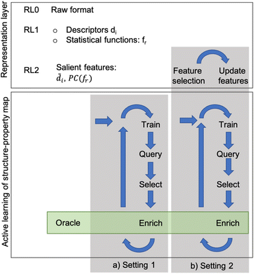
Given a set of microstructures, the aim of the AL workflows is to identify a subset of microstructures that can be used to train a SP model that is accurate over the full dataset. Very generally, we consider the SP relationship to be a regression model between some microstructure features and a desired property of interest. Fig. 1 depicts the AL workflow with two different settings for the active learning pipeline (with and without automated feature selection). AL accompanied by a regression analysis is a semi-supervised learning method that labels data incrementally during the training phase. The AL algorithms select the next sample based on the likely improvement in the model, label that sample using high-fidelity simulations (usually called the oracle), and then update the data pools. The choice of microstructure representation and consequent reduction in dimensionality is critical in influencing the AL performance.

Fig. 1 Workflow: given the dataset of L microstructures and two representations (vector of descriptors and two-point correlations), find the salient features of the target properties and the associated SP relationship using active learning.

In this work, three levels of microstructure representation are employed (see Fig. 1) as outlined in our prior work.² The first transformation (RL0 → RL1) converts microstructures in the raw format (RL0) into an alternative representation (RL1), represented by either graph-based descriptors or statistical functions (two-point correlation functions). The transformation from RL0 to RL1 ensures that the inherently high dimensionality of RL0 is reduced whilst preserving data invariance. Further dimensionality reduction is still beneficial and this work uses feature engineering to achieve this (as shown in Fig. 1). Ideally, the dimensionality reduction is executed at a single instance at an early stage of the workflow (setting 1 in Fig. 1). However, in some instances, the feature engineering may require continuous updates with a set frequency (setting 2 in Fig. 1). Thus, in this paper, AL workflows use two different configurations: setting 1 with feature engineering only at the initial stage and setting 2 with continuous cycles of feature engineering during the workflow. In setting 1, the assumption of prior knowledge of the salient features informs the subselection of descriptors, or for the two-point correlation functions, a Principal Components Analysis (PCA) further reduces the dimensionality of the data. In setting 2, no prior knowledge is assumed, and feature selection occurs on the input space with a specified frequency. Setting 1 is used for both microstructure representations (descriptors and statistical functions), while setting 2 is applied only to the descriptor-based representation. Nevertheless, in both configurations, during each iteration, the surrogate model is retrained, the pool of candidates is queried, the sample is selected for the oracle to evaluate, and then the training data pool is updated for the next AL iteration.

Below, we describe four critical elements of the workflow: the microstructure representation that defines the input to the model, the oracle that labels the microstructure with the true label, the surrogate model of the microstructure-property map and the sampling strategies.

1.2 Microstructure representations

Formally, the input raw data (i.e., image data) consists of L microstructures as , where microstructure X_i is represented by a (n_x × n_y) bitmap (or n_x × n_y × n_z bitmap for 3D microstructures) with bitmap pixel X_i(x, y) ∈ {0, 1} (X_i(x, y, z) ∈ {0, 1} for 3D) at position (x, y) (or (x, y, z) for 3D). The raw data is transformed into two mathematical representations: graph-based descriptors and a two-point correlation function. The set of descriptors is typically application specific³ but are physically meaningful, explainable, and interpretable. Examples include volume fractions, interfacial area per unit volume, connected components density, average domain sizes, tortuosity of the paths, and percent contact area with boundaries. Formally, each descriptor is denoted as d_i and constitutes the vector of descriptors of a microstructure:where n_d is the total number of descriptors. The dimensionality of this descriptor vector is usually much smaller than the dimensionality of the input microstructure and can be further reduced to the vector of salient descriptors D̃ = {d₁, d₂, …, d_ñd} of length ñ_d (<n_d). The salient descriptors are determined through the method of feature selection. We refer to our prior work⁴ for a detailed description of these descriptors and ESI† for the list of descriptors (Table 1 in ESI†). The descriptors are computed for each microstructure, and descriptors subset is used as the feature vector, γ, in the surrogate model (see Subsection 1.4).

Table 1 Comparison between two case studies in terms of number of microstructures, dimensionality of the representation layers

	OPV 2D with known features	OPV 2D with unknown features	Elastic 2D	Elastic 3D
# Microstructures	1708	1708	2000	8900
# Microstructures used in AL	500	500	800	1600
Dimensionality RL0	401 × 101	401 × 101	51 × 51	51 × 51 × 51
Dimensionality RL1	21	21	51 × 51	51 × 51 × 51
Dimensionality RL2	5	8–9	15	15

---

For the second representation, we use two-point spatial auto-correlations (also known as two-point statistics). For the two-phase material system under consideration, only one auto-correlation of the electron-accepting phase is needed.^5,6 Consider a microstructure, X_i. Let m_s denote this microstructure as an array, where s indexes each pixel, and the values of m_s reflect the volume fraction of one phase in the pixel s. In the microstructures considered in this work, each pixel is fully occupied by one of the two phases present in the microstructure. Hence, m_s takes values of zero or one. The auto-correlation of interest is defined as:

where f_r denotes the auto-correlation array indexed by a set of discrete vectors r. The total number of valid placements of the discrete vector r used in evaluating the spatial statistics is denoted as S_r,^7,8 and F_i corresponds to auto-correlation array of microstructure X_i in . The size of the auto-correlation array of microstructure is of the same size as the input microstructure and can be further reduced through dimensionality reduction techniques. In this work, similar to our prior work,² the principal component analysis is used to determine the R principal component (PC) bases that become the feature vector, γ, used in the surrogate model in Subsection 1.4.

1.3 Oracle of microstructure sensitive properties

In this work, the property of the microstructure P is computed using physics-based models – usually called the oracle – that we consider as the ground truth. Typically, the cost of property evaluation is high, which warrants the need for AL workflows.

1.4 Surrogate model of microstructure–property relationship

The central element of the data-driven approach is the model used to represent the SP map. In this work, we use Gaussian process regression (GP)⁹ due to the inherent uncertainty measures associated with the model predictions used in the sampling (see the next subsection). The regression model M(γ) is specified by its mean function m(γ) and covariance function (or kernel) k(γ, γ′), of the GP, where γ and γ′ are the vectors of salient features of the input microstructure. Based on the representation layer RL1 used, the data points γ and γ* correspond to the vectors of salient descriptors or the vectors of R principal components for statistical function representation – as explained in the previous subsection. The regression model is not only used to predict the properties but also to estimate the uncertainty of property prediction on the query point γ*:and the variance of the predicted value:where K_*N denotes the vector of covariances (kernel values) between the query point γ_* and all N training points, P_N is the vector of all properties in the training set of size N, K_NN is the matrix of covariances (kernel values) evaluated on all pairs of training points. σ² is the Gaussian noise, and I is the identity matrix. In this work, Matern kernel and zero mean function have been used to calculate the covariance function of the model.

1.5 Pool-based sampling strategies

Given the microstructure representation, the surrogate model, and the general workflow of active learning, we close this section by describing pool-based sampling strategies. Pool-based sampling is the scenario where a pool of unlabeled data points exists, and at each iteration, additional data points are selected from that pool and labeled. Among the pool-based sampling strategies, we investigate (A) uncertainty-based sampling and (B) coreset sampling and compare them with random sampling that serves as a baseline. The strategies differ in terms of the criterion used to choose the most beneficial unlabeled point.

(A) Uncertainty-based sampling is one of the most commonly used strategies in active learning settings. The data point exhibiting the highest variance when evaluated by the surrogate model is chosen to be labeled by the oracle and then added to the training data pool:

where γ_* is the selected point, and V_T is the vector of variances for all unlabeled T points, where the variance is computed using eqn (4). As a reminder, query points correspond to all T = L − N unlabeled microstructures. Each unlabeled data point is evaluated using the most recent version of the structure–property Gaussian process model to compute the variance of the predicted property.

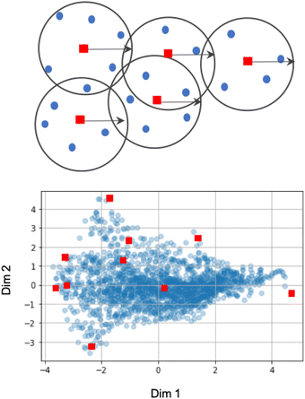
(B) Sampling based on the coreset selection problem is closely related to choosing the optimal subset of points. Intuitively, the coreset is a succinct, small summary of large data sets, so solutions found using the small summary are competitive with solutions found in the full data pool. It has been shown that a sparse greedy approximation algorithm can be used to approximate the corset problem selection,¹⁰ which is an NP-hard problem.¹⁰ demonstrated the utility of the greedy algorithms by minimizing the coreset radius, defined as the maximum distance of any unlabelled point from its nearest labeled point. Such an example coreset is depicted in Fig. 2. The top panel shows the sketch of the coreset concept, highlighting the radius for each coreset element (red points) approximating the surrounding points (blue points). Determining the coreset is an optimization problem that is also problem-dependent since the selection of the summary points needs to be evaluated in the context of the entire data pool. For that reason, approximation approaches based on distances and greedy sampling have been proposed.¹⁰ In essence, the aim is to identify the points that are the farthest away from all previously selected samples. As a consequence, the diversity of sampled points increases. The bottom panel of Fig. 2 demonstrates the low-dimension space for our input space of the first case study. Each blue point in the panel corresponds to one microstructure, where coordinates correspond to the first two PCs learned from the descriptor-based representation. The red points indicate the first points selected by the coreset sampling method. Note the balanced selection of the point in the low-dimensional embedding space, with points being selected uniformly across the entire microstructural two-dimensional subspace.

Fig. 2 Schematic of coreset concept where each red square represents the neighboring blue points within the circle of radius shown (top panel) and the visualization of example coreset points of microstructure dataset used in this work (bottom panel). In both panels, the coreset points are marked red and represent the neighboring points. In the bottom panel, each point denotes one microstructure, where coordinates correspond to the first two PCs of descriptor representation.

In this work, we investigate three greedy approximations of the coreset selection for sampling strategies: greedy sampling on the inputs (GSx), greedy sampling on the output (GSy), and improved greedy sampling (iGS) that uses both input and output.^11,12 The major difference between them is the distance calculation between points that involves computing the distance only in the input space, only in the outputs space, and both spaces. Below, we provide more details:

• GSx only considers the input space of data and chooses the points by computing the Euclidean distance between the labeled data points and unlabeled data points. The microstructures with the largest distance from the current labeled data points will be selected as the next point that needs to be labeled:

where Δ^γ_ij is the matrix of distances between labeled data points and unlabeled data points, γ_i and γ_j are the labeled data points and unlabeled data points, respectively. As an outcome, γ_* is selected for labeling. Intuitively, this is the point that is the farthest away from N already labeled points, where N = T₀ + T. The size of the matrix Δ_ij is N × (L − N). Similar to the previous sampling strategy, γ corresponds to the vector of salient descriptors or the vector of R PCs of the statistical function.

• GSy uses a similar criterion, but it computes the distance between the output of the regression model. Because for the unlabeled data points true value of the property is not available, the most current regression model is used to estimate the properties. Formally, the microstructure for labeling γ_* is determined using analogous criterion:

where Δ^P_ij is the matrix with distances between properties of labeled data points and unlabeled data points, P_i and . Specifically, P_i are true values for labeled data points, and are the predicted properties on unlabeled data points.

• iGS integrated GSx and GSy with the following criterion:

where the element-wise product of two distance matrices from the previous samplings is used to choose the next microstructure for labeling, γ_*.

Finally, we contrast the above strategies with random sampling, where the points are added to the training set randomly. Random sampling does not belong to the active learning type of algorithm, but we include it as a baseline for this work.

1.6 Active learning for regression

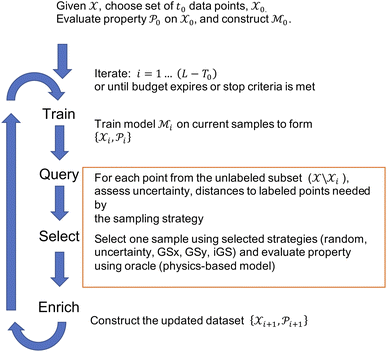
Given the initial raw data set (microstructures) and property of the microstructures, the initial regression model is calibrated using randomly selected T₀ data points. In each iteration of active learning, one microstructure is evaluated for the target properties by the oracle and then added to the data pool used to update the SP model – as outlined in Fig. 3. At a given iteration i, T = i + T₀ labeled points are used for model recalibration. The process continues until the budget expires or other end criteria are reached (e.g., set tolerance on uncertainty, the model accuracy, etc.).

Fig. 3 The workflow of active learning method: and is the dataset with microstructures and the initial data set of raw microstructures, respectively. The property of interest is evaluated at the initial pool of microstructures . The initial dataset refers to the raw microstructures, but in practice, the model uses either the vector of descriptors or a finite number of PCs transformed from the statistical function representation. The regression model is calibrated at any iteration i.

1.7 Active feature selection

Active feature selection means the salient features are updated as a part of an active learning campaign. In such a scenario, the labeled data pool is iteratively increased following steps from Fig. 3, and the salient features are updated. With the specified frequency, ΔT, the feature selection method is performed on the labeled pool to update the salient features. Consequently, the regression model is updated at each iteration of the active learning campaign as more points are added. But input feature space (salient features) can change as well, depending on the outcome of feature selection.

2 Results

In this work, we consider two case studies with different properties. The first case study considers the short circuit current of solar cell devices with a moderate dataset size of two-dimensional microstructures. The second case study considers the effective stiffness parameter of composite microstructures. In the second case study, two and three-dimensional microstructures are analyzed. In both cases, one microstructure and its property constitute one data point for building and validating the desired surrogate model.

2.1 Organic solar cells device property and spinodal decomposition dataset

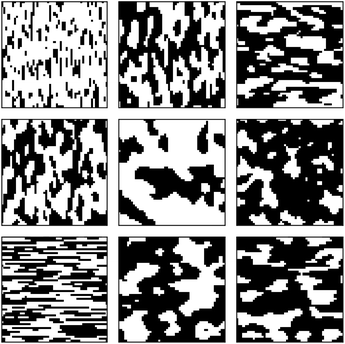
The first case study considers constructing SP maps for organic photovoltaics (OPV) applications. This dataset consists of 1708 OPV microstructures generated using a Cahn–Hilliard equation solver.¹³ The microstructure is a two-dimensional, two-phase microstructure of size 401 × 101 pixels and it constitutes the active layer of OPV. Fig. 4 depicts example microstructures used in this work. Microstructure consists of two phases, one as an efficient electron donor and the other as an efficient electron acceptor material. The active layer being modeled is sandwiched between two electrodes: an anode and a cathode. Each microstructure in this dataset is annotated by one property, the short circuit current – J_sc. The J_sc is derived using a physics-based computational model that is computationally demanding. The model solves the excitonic drift-diffusion equations. The model focuses on the charge transport through the microstructure (based on a well-studied material system, P3HT:PCBM blend‡ mixture). It solves the spatial distribution of excitons, electrons, holes, and the electric potential across the active layer of the OPV device. This microstructural dataset is of moderate size, but predicting properties required substantial resources.¹⁴ Additional details on data generation and the computational models are presented in our prior work.^13,15 The short circuit current is considered the ground truth values for J_sc, and its values for individual microstructures are used to calibrate data-driven SP models examined in this paper.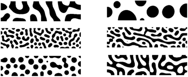

Fig. 4 Example microstructures generated for the OPV active learning workflow. Each microstructure is of size 401 × 101 pixels.

2.2 Elastic properties and composite data

The second case study considers the elastic property of composite microstructures for 2D and 3D data sets. Both data sets use similar methods for generating the microstructures^16–19 as well as computing the effective property.^20,21 In the 3D case, 8900 microstructures are generated with grid sizes of 51 × 51 × 51. In the 2D case, 2000 data samples are generated with grid sizes of 51 × 51. Fig. 5 depicts the examples of microstructures from the 2D dataset. The dataset contains both isotropic and anisotropic microstructures. The figure shows examples of lamellar-like microstructures as well as more equiaxed grains. The discrepancy in dataset size is related to the much larger dimensionality of the microstructure in 3D, which demands larger datasets for model calibration.

Fig. 5 Example microstructures generated for the 2D elastic property active learning workflow. Each microstructure is of size 51 × 51 pixels. In this work, lamellar-like microstructures are aligned in either vertical or horizontal directions.

The material system used in this study is a high-contrast elastic composite microstructure, which leads to a longer range and more complex non-linear interactions at the micro-scale. The micro-scale constituents (only two phases in this work) are assumed to exhibit an isotropic elastic response. A contrast of 50 is chosen by setting the Young moduli of each phase to E₁ = 120 GPa and E₂ = 2.4 Gpa, respectively. However, Poisson ratios are kept the same for both phases, i.e., ν₁ = ν₂ = 0.3. The targeted property of interest is selected as the effective stiffness parameter, C^eff₁₁.

2.3 Technical details

In this work, two relatively inexpensive approaches are used to featurize the microstructures. Firstly, the GraSPI software⁴ is used to compute descriptors for the OPV data. GraSPI computes the graph representation of the microstructure and then generates twenty-one descriptors for each sample.²² In the case of the OPV data set (constructed using the GraSPI approach), the run times are approximately two seconds to reduce a microstructure of size 400 × 100 to 21 descriptors. The short circuit current of organic solar cells is the property of interest and it is computed using drift-diffusion model. The analysis is performed only for two-dimensional microstructures due to the prohibitively high computational cost of three-dimensional analysis. The simulation for each 2D microstructure takes around 20–40 minutes on four CPUs and 8 GB of memory. In contrast, a 3D analysis of the first case study for a single microstructure takes 12 h on 36 CPUs.

Secondly, the PyMKS (Materials Knowledge System in Python) software is used to compute the two-point correlations function and subsequent dimensionality reduction on the elastic data sets.²³ Only the first 15 PC scores are used to calculate the subsequent GP model. For the 2D case, the generate_multiphase function from the PyMKS package²³ implements the synthetic generation. The process involves a random field with a Gaussian blurring filter that generates specified microstructure sizes with a normal distribution. The 2D synthetic microstructure has a 10-fold size difference between the coarsest and finest microstructure matrix. The 3D synthetic generation method is analogous to the Gaussian filter method available in the PyMKS package. However, a prior dataset is used from previous work²⁴ due to the high computational cost of regenerating the associated property predictions.

In the case of the elastic data sets, the calculation takes 5 seconds using 10 cores to compute both the two point correlations and PCA analysis for 2000 samples of size 51 × 51. For the 3D data (8900 samples of size 51 × 51 × 51), the same calculation takes 269 s using 10 cores. The effective stiffness (a single value for each microstructure) is calculated using the Sfepy finite element tool.²⁵ The solve_fe function (which uses Sfepy internally) from PyMKS is used to generate the data.²³ Details of the simulations can be seen in prior work.^26,27 The simulation for each 3D sample takes around 15 min with 4 CPUs and 32 GB of memory. This computational cost is reasonable. The Jupyter Notebooks and code implementation for generating the microstructure data and calculating the active learning curves are available.²⁸

2.4 Active learning settings and data split

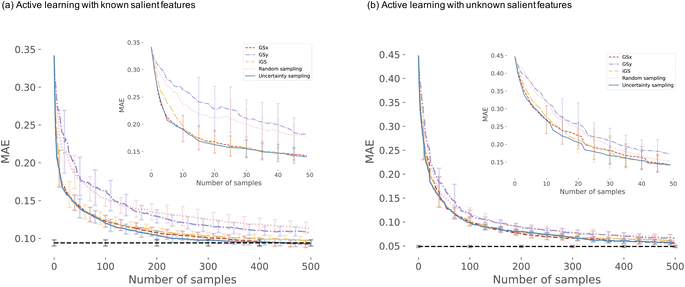
During the generation of the active learning (AL) curves, data is standardized, and an 80/20 train/test split is used. The train/test split is reordered for each repetition of the AL curves. Initially, T₀ = 10 samples are randomly assigned to the initial pool of samples, and then the training set is iteratively increased. The final number of pool samples is 500 for the OPV data set. It is 800 and 1600 for the 2D and 3D elastic data sets, respectively. The performance reported for each AL curve is the mean value at each iteration using 20 repetitions for all data sets. The same initial pool of data and train/test split is used across each of the AL techniques for any given repetition. This guarantees that the mean averaged curves (shown in the figures) have the same starting location and are trained with the same starting conditions.

2.5 Active learning curves for the OPV 2D dataset

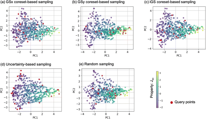
We start the results with the learning curves for various sampling strategies. The learning curve depicts the evolution of the model performance as the size of the training size increases. Fig. 6 shows two panels of model performance for the five sampling strategies for the first dataset and OPV device performance. The mean absolute error (MAE) is depicted for all sampling strategies. For each dataset, the data is standardized. Fig. 6(a) shows curves for active learning with known salient features (setting 1). Fig. 6(b) depicts the learning curves for active feature selection with salient features learned during the active learning campaign (setting 2).

Fig. 6 Active learning curves for the OPV dataset for (a) setting 1 active learning with known features: note that the uncertainty-based sampling requires the least number of data points to construct the model with optimal accuracy; (b) setting 2 active learning coupled with the feature selection. The top plot in both panels depicts the average performance of 5 sampling strategies for the first 50 iterations of the active learning campaign. The results are obtained from 20 repetitions of the workflow. In both panels, the black dashed line denotes the optimal model derived from 20 repetitions of 80/20% split of all the data. The error bars represent a single standard deviation.

In setting 1, we choose 5 features: d₃, d₁₁, d₂₀, d₂₁, d₂ as the salient features (see Table 1 in ESI† for the complete list). After 50 iterations, three sampling strategies (iGS, GSx, and uncertainty sampling) converge to the models of comparable accuracy with MAE = 0.14. Moreover, at this point, the uncertainty of the MAE is small (±0.011). The other two sampling strategies converge much slower (random and GSy) than the top strategies. The variance for GSy and random sampling is also higher than the remaining three strategies. Moreover, after 50 iterations, GSy showed performance and a rate of convergence comparable to that of random sampling. We attribute this high uncertainty of GSy sampling to the limited scope of information used for model calibration with data points taken from the narrow range PC2 of the input space. Results presented in Fig. 7(b) illustrate this observation. Red points highlight the microstructures projected to the two PC subspaces that have been selected after 20 iterations of the active learning strategy. For GSy, the points are selected from the wide range of PC1 subspaces but are centered around central values of PC2 subspaces. Such distribution of the microstructural points is aligned with the strategy used, as GSy strategy chooses the points that are the farthest away from already selected points in the property space. The color of the point codes the value of the property, with the red points spanning the wide range of the property values. In contrast, for the iGS sampling strategy (Fig. 7(c)), the red points are distributed fairly uniformly across the two PC subspaces and the property space. Moving to uncertainty sampling (Fig. 7(d)), points are selected from the outskirts of the input space. This is because uncertainty sampling chooses the next points based on the uncertainty of the model prediction. In the early stages of the GP model calibration, the points on the boundaries of the input space typically are assigned with relatively high uncertainty. Consequently, with the GP's default settings, in the early stages of exploration, these points are more likely to be selected for labeling. In our comparative analysis, the tendency to select points for exploration at the boundaries affects the performance of this sampling strategy. The same observation can be made for distance-based sampling (GSx, GSy, iGS) because, in the initial iterations, distance-based samplings (like coreset) tend to choose the points with the longest distance from those already selected. Closing with the random sampling, points are selected randomly in the input space without any clear pattern – as visualized with red points in Fig. 7(e). The latent space distribution for setting 2 mimics the results presented in Fig. 7 and, hence, these results are included in the ESI.†

Fig. 7 Visualization of query point selection using different sampling strategies: (a) GSx, (b) GSy, (c) iGS, (d) uncertainty sampling, and (e) random sampling with known salient features. Each panel highlights 20 points selected using a given strategy (marked red), and also includes remaining points that are color-coded using the property of interest-J_sc. Note that each point corresponds to one microstructure projected into the first two principal components of descriptor-based representation.

To provide a more quantitative analysis of the sampling strategy, three metrics are selected (definitions are included in the ESI†):

(i) Wasserstein distance between two data distributions: the dataset at a given iteration and the complete dataset. This metric provides insight into the representativeness of the current subset of data. With the increased number of samples, the distance should decrease. The short distance between data distribution is expected is data pool is representative of entire dataset.

(ii) The entropy of the variable (microstructure dataset) is a measure of the variable's uncertainty or information content. When the entropy of the variable is low, samples in the subset are relatively similar; when the entropy of the variable is high, the samples in a given dataset are diverse.

(iii) Mean uncertainty is defined as the mean, standard deviation of property prediction over all unselected data at each iteration. A GP regression model is used to compute the standard deviation of predicted property for each unselected sample and then averaged. Intuitively, when uncertainty is high, the model offers an exploratory opportunity.

Fig. 8 visualizes a comparison of five sampling strategies used in this work on the descriptor-based microstructure representation. We start the analysis with the Wasserstein distance between the current distribution of microstructure and the complete microstructural dataset. The distance is computed for the input space only – the low dimensional 3 PC subspace of the descriptor-based microstructural representation. The shortest distance we observe for the random sampling and the longest for the uncertainty-based and GSx samplings. This agrees with the intuition. Random sampling chooses the points that are representative of the entire population; hence, the distance is short. For the uncertainty sampling and GSx sampling, the most uncertain points and the most unrepresentative points in the input space are chosen; hence, the distance is long. However, iGS is the only sampling strategy to yield intermediate Wasserstein distances.

Fig. 8 The three metrics used to assess the active learning algorithms and random method when salient features are known – setting 1. Each curve represents the mean of 20 repetitions for 500 iterations. The error bar represents a single standard deviation. In the panel (a), Wasserstein distance is calculated for 5 different sampling techniques. In the panel (b), the entropy for the salient feature vectors is calculated. The entropy for the whole data set is shown as the dashed line. In the right (c), the uncertainty of property prediction is calculated. The error bars represent a single standard deviation.

Moving now to the entropy of the microstructure distribution, we see a different grouping of the sampling strategies. Uncertainty-based and GSx sampling strategies exhibit the largest entropy, with the maximum value at around 100 samples. GSy and random sampling show the lowest entropy that very quickly converge to the value of the entire dataset. Finally, iGS shows an intermediate trend – which is a similar ranking to the Wasserstein distance analysis. We attribute the highest entropy values of the GSx and uncertainty-based samplings to the inherent feature of selecting points from the underexplored regions of the input space – as demonstrated in Fig. 7. Sampling iGS also chooses the underexplored regions of the spaces and balances information about input and output space.

We close with the analysis of the last metric – the mean uncertainty of the property prediction – see Fig. 8(c). Uncertainty-based and GSx sampling show the lowest value of the uncertainty of the property prediction, while GSy and random show the highest values of this metric. Sampling iGS exhibits the intermediate trend – as is consistent across all three metrics. The low uncertainty value in uncertainty-based sampling agrees with the intuition, as this sampling aims to choose points that balance exploration and exploitation and minimize the uncertainty of the prediction. The reason to calculate this metric is to assess how other metrics compare with each other. The analysis of the trends for three metrics indicates that iGS offers a good balance between representative, diversity, and uncertainty of the data points selected for the labeling. In three panels of Fig. 8, iGS places in the middle.

Next, we analyze the results for setting 2 (Fig. 6(b)), where the feature selection is applied for every 10 iterations. The feature selection technique used in this work is the embedded method – Random Forest (RF). As a consequence, the input features may change with this frequency. The learning curves (Fig. 6(b)) demonstrate that iGS is still the best strategy, with the MAE converging the fastest among the five sampling strategies. However, compared to active learning with known salient features (Fig. 6(b)), the overall converging rate in this setting is slower than in the left panel. Moreover, the uncertainty of active learning strategies is higher than in setting 1 (0.012 compared to 0.0093). The most important features selected by active learning methods become stable after about 60 iterations, which is consistent with learning curves in Fig. 6. The salient features selected by the feature selection method are not stable at the beginning stage of active learning (due to the small number of samples selected), and the learning curves reach a plateau at a higher number of iterations compared to other strategies. The changes in the selected features are provided in the ESI – see Fig. S2.† The evolving salient features also have a direct impact on the converging rate of the learning curves in setting 2. Initially, sixteen features are selected for the GP model calibration. With the subsequent iterations, the required number of features decreases to nine (which is higher than assumed in setting 1). The increasing number of features has a direct impact on the distance calculations in the corset-based sampling strategies (GSx, GSy, iGS) and on the GP model calibration as the number of dimensions increases. Nevertheless, all sampling strategies converge to a low MAE error of the model. The differences between the learning curves are small, which suggests that when salient features are unknown priori, even with the simplest sampling strategy, the model reaches low error fairly quickly. Our results suggest either GSx or iGS sampling as the best strategy.

2.6 Active learning curves for the elastic 2D and 3D datasets

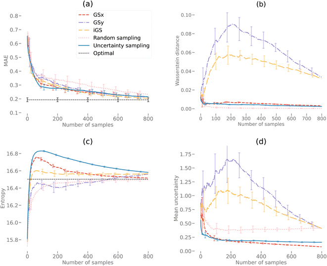
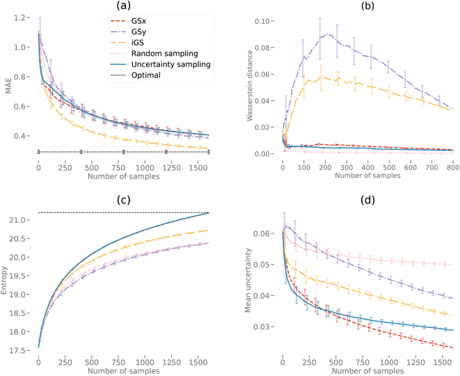
Fig. 9(a) and 10(a) display the AL curves for the 2D and 3D data sets, respectively. Both figures show the iGS strategy performing well, but there are some significant differences. In particular, The iGS method outperforms all other sampling methods for the 3D data set. Notice that in both cases, the GSx method performs well over the initial regime (first ≈ 30 iterations) but then tails off considerably. Initially, the GSy method performs poorly but then begins to accelerate faster than GSx at later iterations. In both cases, the GSx method follows the trajectory of the uncertainty sampling method quite closely. This indicates that the GSx method is very similar to uncertainty sampling for these data sets. This is confirmed by plots (b), (c) and (d) for both Fig. 9 and 10 discussed in the following paragraphs. As the iGS method embeds both the GSx and GSy methods within its algorithm, it can benefit from both sampling methods at different regimes along the AL curves. During the initial phase, the iGS method uses GSx and keeps parity with uncertainty sampling but then starts to use the acceleration from GSy to move past uncertainty sampling. This occurs in both the 2D and 3D data, but earlier and much more significantly in the case of the 3D data set. For the 3D data set, the iGS method is the only method to approach the optimal accuracy after 1600 iterations of AL.

Fig. 9 Active learning curves for the 2D elastic data set (2000 samples of 51 × 51 voxels). Random sampling is included as a reference. Each curve represents the mean of 20 repetitions, each with a randomly selected 20% test hold-out data set. The error bars represent a single standard deviation. Subplot (a) displays the mean absolute error (MAE) versus the number of samples for different sampling techniques. The “optimal” curve is not an active learning curve but a single value derived from 20 repetitions of an 80/20% train/test split of all the data. It represents the optimal value that can be reached by the active learning curves. Subplot (b) displays the Wasserstein distance versus the number of samples. The Wasserstein distance is calculated as using both the PCA scores for the sample subset at a given number of samples and the entire PCA data set. Subplot (c) displays the entropy estimate versus the number of samples calculated using a kernel density estimator. This gives an estimate of the variance of the selected sub-spaces. The black dotted line shows the variance for the entire data set. Subplot (d) displays the mean uncertainty versus the number of samples calculated from the GP model.

Fig. 10 Active learning curves for the 3D elastic data set (8900 samples of 51 × 51 × 51 voxels). Random sampling is included as a reference. Each curve represents the mean of 20 repetitions, each with a randomly selected 20% test hold-out data set. The error bars represent a single standard deviation. Subplot (a) displays the mean absolute error (MAE) versus the number of samples for different sampling techniques. The “optimal” curve is not an active learning curve but a single value derived from 20 repetitions of an 80/20% train/test split of all the data. It represents the optimal value that can be reached by the active learning curves. Subplot (b) displays the Wasserstein distance versus the number of samples. The Wasserstein distance is calculated as using both the PCA scores for the sample subset at a given number of samples and the entire PCA data set. Subplot (c) displays the entropy estimate versus the number of samples calculated using a kernel density estimator. This gives an estimate of the variance of the selected sub-spaces. The black dotted line shows the variance for the entire data set. Subplot (d) displays the mean uncertainty versus the number of samples calculated from the GP model.

Fig. 9(b) and 10(b) display the Wasserstein distance calculations. Note that we are only considering the Wasserstein distances from the optimal transport in the PCA subspace of the input microstructures, not the output space. The GSy method has the largest distance from the data at a given iteration to the complete data set. This is unsurprising as the GSy method is only sampling using information about the property (output space) – not the microstructure (input space). In both cases, random sampling is the best method to generate a model close to the PCAs from the full data set in the same way that random sampling is a good way to reconstruct a probability density function. In Fig. 9(b) during the very early iterations (<10), the Wasserstein distance for the iGS method decreases, indicating that it is sampling based on the PCA space. After this early stage, it samples from a mixture of the PCA and output space (switching between GSx and GSy) and then eventually mostly from the output space.

Fig. 9(c) and 10(c) display the entropy calculations. In essence, this is a measure of how even or flat the microstructure distributions for the selected samples are when projected into the PC subspace. In both cases, uncertainty sampling creates the largest entropy, indicating that it is optimizing for this property in particular. Uncertainty sampling is optimizing samples based on capturing the support of the data distribution rather than the values of the distribution in that range. Note that some sampling methods overshoot the overall entropy value in the 2D case but fail to overshoot in the 3D case after 1600 iterations. However, we anticipate that uncertainty sampling and GSx will overshoot at just after 1600 iterations in the 3D case. Both GSy and random sampling have lower entropy values than the other sampling methods as both sampling methods are not optimized for an even or flat PDF, but in the case of random sampling, only model the overall PDF (capturing the values or shape). Unsurprisingly, the iGS method lies between the GSx and GSy methods for the entropy calculation (as indeed it does for the Wasserstein calculation) demonstrating how this method balances between both approaches to achieve better overall accuracy.

Fig. 9(d) and 10(d) display the mean uncertainty calculated from the GP model. Clearly, at early times, uncertainty sampling decreases the uncertainty of the predicted model at the fastest rate. In the 2D case, uncertainty sampling flattens out after the initial decrease. This is due to the calculated uncertainty calculated by the GP model being very even across all the samples. This makes it difficult to optimize the AL via uncertainty only. In the 3D case, the overall uncertainty is much higher than in the 3D case. After 1600 iterations each method is still decreasing its predicted mean uncertainty. In both the 2D and 3D plots, the GSx method decreases the uncertainty below that of uncertainty sampling. This indicates that the maximum uncertainty value is no longer the best choice for the next sample in the AL. This is due to the uncertainty becoming more even across samples at later iterations. Spatial configuration considerations of the PCA and output spaces become more efficient at decreasing the uncertainty (and increasing model accuracy) at the later stages. Note that, as in the previous plots, the iGS method achieves a balance between the GSx and GSy methods.

2.7 Comparative analysis of two case studies

Two case studies involve different types of microstructure (composite vs. spinodal), dimensionality (two- and three-dimensional), and properties (elastic and electronic). Moreover, two separate microstructures representations are evaluated: graph-based descriptors derived from a graph representation of the microstructure and two-point correlation functions. This work is part of a more extensive study, with a more detailed comparison between two representations provided in our prior work.² This paper aims to ask the question of the minimal number of samples needed to construct a robust SP map given a library of microstructure. Below, we provide a brief comparison in terms of data available and the dimensionality of three representation layers (Table 1). We also compare the observation made for two case studies in terms of a minimal number of samples needed (Table 2).

Table 2 The number of iterations required to reach an 80% improvement, i_cutoff, from the initial accuracy value towards the optimal accuracy value. Values in parentheses represent the fraction of the dataset represented by the number of samples

Sampling method	OPV 2D with known features	OPV 2D with unknown features	Elastic 2D	Elastic 3D
Random	131 (8%)	80 (5%)	454 (23%)	965 (11%)
Uncertainty	45 (3%)	58 (4%)	107 (5%)	1042 (12%)
GSx	48 (3%)	55 (4%)	191 (10%)	1087 (12%)
GSy	142 (9%)	82 (5%)	270 (14%)	937 (11%)
iGS	44 (3%)	60 (4%)	221 (11%)	422 (5%)

---

Table 1 details the data availability and the dimensionality of three representation layers, which provides a comparative analysis of two case studies – OPV 2D and elastic materials. The OPV 2D datasets, with both known and unknown features, comprise 1708 microstructures each, utilizing 500 iterations in active learning (AL). The elastic datasets, with 2000 microstructures for 2D and 8900 for 3D, use 800 and 1600 iterations in AL, respectively. The initial dimensionality (RL0) is 401 × 101 for OPV 2D compared to elastic 2D: 51 × 51, and elastic 3D: 51 × 51 × 51. Subsequent RL1 and RL2 representation layers reduce the dimensionality in OPV 2D, notably to 21 and 5 (8–9 in unknown features setting§). In OPV 2D case, the dimensionality reduction from RL0 to RL1 is through physical descriptors derived from graph-based model. And from RL1 to RL2 is through the feature selection method. Meanwhile, elastic datasets maintain higher dimensions through RL1 (dimensionality remains the same as RL0), and the dimensionality at RL2 reduces to 15 PCs.

Table 2 summarizes the sampling strategies by extracting the number of samples required to observe improvement in the accuracy of the model (80% improvement from the initial accuracy value to the optimal value). The criterion is arbitrary, but it allows comparing the sampling strategies for each case study, as the initial model and optimal model are independent of the strategies taken. The table lists the required number of iterations to achieve the criterion and the corresponding fraction of the complete dataset. For the first case study and OPV-setting 1 (known salient features), our analysis indicates that iGS sampling stands out for its efficiency, requiring the smallest number of iterations. Nevertheless, uncertainty and GSx strategies require a comparable number of iterations. The two remaining strategies, random and GSy, require a significantly higher number of iterations. In setting 2 of the OPV case study (unknown salient features), the AL workflow requires more iteration, but the ordering of the sampling shows a less clear trend. Uncertainty, iGS, and GSx sampling strategies required fewer iterations than random and GSy strategies to reach the criterion. But the difference is minor.

For the second case study, uncertainty sampling is the best approach for the 2D elastic data set requires only half as many iterations to reach an equivalent accuracy as the other sampling methods. In the case of the 3D data set, the iGS method requires less then half the number of iterations as any of the other sampling methods to reach the cutoff accuracy.

In summary, given the varying size of the dataset, the dimensionality of each microstructure, and different properties (two case studies), active learning workflow significantly reduces the number of physics-based evaluations. Our work reports that, on average, 10% of data is needed to calibrate a robust surrogate SP model. Sampling strategies can further reduce the requirement to 3–4% (depending on the case study). Sampling using information about input and output spaces – iGS – offers the best performance across four studies; however, it is the most complex sampling strategy. GSx is worth highlighting as it performs reasonably well. However, it only operates on the input space information and requires no update from the surrogate model. Hence, using GSx, the microstructures can be fairly easily ordered for property evaluation without overhead of property estimation.

3 Conclusions

We presented a comparative analysis of two microstructure representations and five sampling strategies of active learning method on three datasets. We learned that regardless of the strategy or problem, at least 5% of the microstructure library is required to construct a robust data-driven model of a microstructure–property map. This observation is valid for the scenario where a large library of microstructures is available for labeling, and information about the distribution of the microstructures can be leveraged to choose the samples for labeling. Our findings showed that both microstructure representations can be effective in such a small data regime when combined with active learning strategies. However, the dimensionality of the latent space varies. We also learned that the choice of the sampling strategy is agnostic to the representation and problem. Sampling iGS performed the best across all the datasets and microstructure representation selection. We attributed the superior performance of this strategy to the balanced information used about the distribution of data in the input and output spaces.

Data availability

The source code for the analysis is available in two separate GitHub repositories. The source code for the OPV 2D dataset workflow is available in a GitHub repository.²⁹ The source code for the elastic 2D and 3D dataset workflows are available in a separate GitHub repository.²⁸ This repository contains the microstructure data and corresponding responses for both the 2D and 3D datasets. The elastic 2D data is available in the subdirectory 2D/data-gen/data-500.npz, while the elastic 3D data is available in the subdirectory 3D/data_shuffled.npz. The entire software stack required for the elastic 2D and 3D dataset workflow is listed in requirements.txt. The source code for analysis is available in Github: https://github.com/usnistgov/active-learning, https://github.com/hliu56/Active-Learning-Using-variousrepresentations.

Conflicts of interest

There are no conflicts to declare.

Acknowledgements

This work was supported by the National Science Foundation (1906344 and 1910539). BG acknowledges partial support from the NSF 2323716. OW and HL acknowledge the support provided by the Center for Computational Research at the University at Buffalo. BY and SK acknowledge support from NSF 2027105.

Notes and references

1. M. D. Wilkinson, M. Dumontier, I. J. Aalbersberg, G. Appleton, M. Axton, A. Baak, N. Blomberg, J.-W. Boiten, L. B. da Silva Santos and P. E. Bourne, et al. , Sci. Data, 2016, 3, 1–9.
2. H. Liu, B. Yucel, D. Wheeler, B. Ganapathysubramanian, S. R. Kalidindi and O. Wodo, MRS Commun., 2022, 1–9.
3. O. Wodo, S. Tirthapura, S. Chaudhary and B. Ganapathysubramanian, Org. Electron., 2012, 13, 1105–1113.
4. GraSPI: an extensible software for graph-based morphology quantification in organic electronics, 2021, https://github.com/owodolab/graspi.
5. D. T. Fullwood, S. R. Niezgoda, B. L. Adams and S. R. Kalidindi, Prog. Mater. Sci., 2010, 55, 477–562.
6. A. Gokhale, A. Tewari and H. Garmestani, Scr. Mater., 2005, 53, 989–993.
7. A. Cecen, T. Fast and S. Kalidindi, Integrating Materials and Manufacturing Innovation, 2016, 5, 1–15.
8. S. R. Kalidindi, Hierarchical materials informatics: novel analytics for materials data, Elsevier, 2015.
9. C. E. Rasmussen and C. K. I. Williams, Gaussian processes for machine learning, MIT Press, 2006, pp. I–XVIII, 1–248.
10. O. Sener and S. Savarese, International Conference on Learning Representations, 2018.
11. D. Wu, C.-T. Lin and J. Huang, Inf. Sci., 2019, 474, 90–105.
12. D. Stoecklein, K. G. Lore, M. Davies, S. Sarkar and B. Ganapathysubramanian, Sci. Rep., 2017, 7, 46368.
13. O. Wodo and B. Ganapathysubramanian, J. Comput. Phys., 2011, 230, 6037–6060.
14. O. Wodo, J. Zola, B. S. S. Pokuri, P. Du and B. Ganapathysubramanian, Mater. Discovery, 2015, 1, 21–28.
15. H. K. Kodali and B. Ganapathysubramanian, Modell. Simul. Mater. Sci. Eng., 2012, 20, 035015.
16. J. D. Hyman and C. L. Winter, J. Comput. Phys., 2014, 277, 16–31.
17. A. P. Roberts and M. A. Knackstedt, Phys. Rev. E: Stat. Phys., Plasmas, Fluids, Relat. Interdiscip. Top., 1996, 54, 2313.
18. Y. Jiao, F. Stillinger and S. Torquato, Phys. Rev. E: Stat., Nonlinear, Soft Matter Phys., 2007, 76, 031110.
19. Y. Gao, Y. Jiao and Y. Liu, Acta Mater., 2021, 204, 116526.
20. G. Landi, S. R. Niezgoda and S. R. Kalidindi, Acta Mater., 2010, 58, 2716–2725.
21. S. R. Kalidindi, S. R. Niezgoda, G. Landi, S. Vachhani and T. Fast, CMC-Computers, Materials & Continua, 2010, 17, 103–125.
22. D. Jivani, J. Zola, B. Ganapathysubramanian and O. Wodo, SoftwareX, 2022, 17, 100969.
23. D. Wheeler, D. Brough, A. Shanker, B. Yucel, S. Voigt, A. Rossi, A. Cecen, F. Hohman, N. Paulson, A. Lohse, A. Medford, A. Iskakov, S. Kalidindi, A. Castillo, M. Diehl, A. Blekh, M. Whitley, R. Cimrman, E. Popova and S. Mohan, materialsinnovation/pymks: Version 0.4.1a1, 2021,  DOI:10.5281/zenodo.5043652.
24. Z. Yang, Y. C. Yabansu, R. Al-Bahrani, W.-k. Liao, A. N. Choudhary, S. R. Kalidindi and A. Agrawal, Comput. Mater. Sci., 2018, 151, 278–287.
25. R. Cimrman, V. Lukeš and E. Rohan, Advances in Computational Mathematics, 2019, 45, 1897–1921.
26. G. Landi, S. R. Niezgoda and S. R. Kalidindi, Acta Mater., 2010, 58, 2716–2725.
27. S. R. Kalidindi, S. R. Niezgoda, i. Giacomo L and T. Fast, CMC-Computers, Materials & Continua, 2010, 17, 103–126.
28. D. Wheeler, Software for Active Learning Using Various Representations, 2024, https://github.com/usnistgov/active-learning.
29. H. Liu, Active Learning Using Various Representations OPV, 2024, https://github.com/hliu56/Active-Learning-Using-various-representations.

---

Footnotes

† Electronic supplementary information (ESI) available. See DOI: https://doi.org/10.1039/d4dd00073k

‡ P3HT:PCBM is poly(3-hexylthiophene) and 1-(3-methoxycarbonyl)-propyl-1-phenyl-[6,6]C₆₁.

§ The number of features depends on data and algorithm in AL.

---