Machine learning the screening factor in the soft bond valence approach for rapid crystal structure estimation

Abstract

The development of novel functional ceramics is critically important for several applications, including the design of better electrochemical batteries and fuel cells, in particular solid oxide fuel cells. Computational prescreening and selection of such materials can help discover novel materials but is also challenging due to the high cost of electronic structure calculations which would be needed to compute the structures and properties of interest such as the material's stability and ion diffusion properties. The soft bond valence (SoftBV) approach is attractive for rapid prescreening among multiple compositions and structures, but the simplicity of the approximation can make the results inaccurate. In this study, we explore the possibility of enhancing the accuracy of the SoftBV approach when estimating crystal structures by adapting the parameters of the approximation to the chemical composition. Specifically, on the examples of perovskite- and spinel-type oxides that have been proposed as promising solid-state ionic conductors, the screening factor – an independent parameter of the SoftBV approximation – is modeled using linear and non-linear methods as a function of descriptors of the chemical composition. We find that making the screening factor a function of composition can noticeably improve the ability of the SoftBV approximation to correctly model structures, in particular new, putative crystal structures whose structural parameters are yet unknown. We also analyze the relative importance of nonlinearity and coupling in improving the model and find that while the quality of the model is improved by including nonlinearity, coupling is relatively unimportant. While using a neural network showed practically no improvement over linear regression, the recently proposed GPR-NN method that is a hybrid between a single hidden layer neural network and kernel regression showed substantial improvement, enabling the prediction of structural parameters of new ceramics with accuracy on the order of 1%.

---

1 Introduction

In the development of novel materials for various applications, computation-guided design has been acquiring increasing importance. The availability of methods to compute properties and the availability of significant and growing CPU resources in principle permit in silico discovery of new promising materials before more expensive experimental work is engaged.^1–5 Computation-guided design is particularly important for functional ceramics needed in technologies such as electrochemical batteries, fuel cells, electrolysis cells, and other technologies important for sustainable energy generation, storage, and use.^6–10 This includes functional oxides for solid-state ionic applications: solid-state metal-ion batteries (SSB)^11,12 and solid oxide fuel cells/electrolysis cells (SOFC/SOEC),¹³ where the development of novel solid-state ionic conductors for various ions (alkali and alkali earth metal ions for SSB, protons and oxide ions for SOFC/SOEC) is still needed that would possess sufficient ionic conductivity as well as thermodynamic and redox stability and sufficiently low cost.^14–17 All these applications have much in common: for all types of conducted ions, there is a similarity of conceptual frameworks that can be employed for their understanding and design, a similarity of promising types of materials for them, and a similarity of modeling methods that can be used to produce mechanistic insight and to computationally pre-screen and guide the experimental development of new materials. There are also differences due to different mechanisms of ion–host interactions with different conducted ions. There is a vast design space, in particular, for mixed and doped oxides, which likely contain efficient solid electrolytes. The challenge is getting to the right material in that space. Computational prescreening and mechanistic insight-directed search are ways to achieve this.

Density functional theory (DFT)^18,19 is in principle sufficiently accurate to ascertain the required properties of a ceramic material with a putative composition and (crystal) structure. It can provide mechanistic insights, control, and resolution not easily achievable experimentally, but the relatively high computational cost of DFT calculations makes prescreening of all conceivable structures, let alone all ionic conduction paths, in a wide range of candidate materials too tedious. Such prescreening can in principle be done at the force field level if a force field framework is available that can be used for a wide range of ceramics and provide sufficient accuracy without requiring refitting of the force field for every new composition and structure. Most promising material candidates can then be subject to more detailed analysis with DFT and ultimately experimental verification.

The soft bond valence approximation (SoftBV) developed by Adams and co-workers provides such a framework.^20–22 It is a type of two-body force-field approximation that incorporates assumptions about the physics of bonding interactions. It is based on the bond valence approximation²³ and the inclusion of screened coulombic interactions, which is appropriate for sufficiently ionic bonding. In this approach, one introduces a Bond Valence Site Energy (BVSE) which is a sum of contributions from all cations i^21,22

where the sum over j is the sum over anions, is bond valence at the interatomic distance of R_i,j between i and j ions, s_min,ij = s_ij|_Rij=Rmin,ij is the value of s_ij at the “equilibrium” geometry described by interatomic distances R_min,ij. D_0,ij, R_0,ij, b_ij, and screening factor (sf) are parameters. r_i are ionic radii. q_i are effective charges of the ions. Here and in the following, we use indices i for cations and j for anions unless stated otherwise. The sum in eqn (1) is taken over ion's N_j nearest neighbors (typically first coordination sphere defined by a cutoff radius R_cutoff,ij which is another parameter) and all cations whose number is M. The choice of summation as a function of the atomic environment gives it a flavor of a reactive force field. Coulombic interactions, contrary to common force fields, are only explicitly included for repulsion between effective charges q_i (see below) and are screened (controlled by sf). In eqn (1), strictly speaking, only sf is an unconstrained free parameter. Relations have been established among the other parameters. The parameters b_ij can be expressed via ionic softness (inverse of hardness²⁴) σ of the anion A and cation C, where a_i are coefficients fitted based on empirical HSAB (hard and soft acids and bases) concept.²² A consistent set of relations between parameters has been developed^21,22,25,26 by making the SoftBV force field agree with known structures and other known force fields such as the universal force field (UFF).²⁷ According to those works, the bond breaking energy D_0,ij is related to b_ij and the oxidation state V_i,j as:^21,25where κ is a coefficient (κ = 14.4 eV Å⁻¹ if these units are used), c is related to the maximum angular momentum of the valence shell of the cation (c = 1 for s- and p-block elements, and 2 for d- and f-block elements), and n_i, n_j are the principal quantum numbers of the cation and anion.^21,25R_0,ij can be thought of as the bond length resulting between the anion and cation when the cation contributes one valence to the anion;²⁸ it is related to other parameters as^21,25,26where γ_1,2 are coefficients and N_C is the coordination number. When matching to UFF, there is also a relationship between D_0,ij, R_0,ij, and b_ij:²⁶

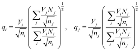
The effective charges q_i and q_j of anions and cations in eqn (1) are typically calculated as^21,25

This ensures, in particular, the overall charge neutrality. A relationship between R_cutoff,ij and other parameters has also been proposed:²²

where k is an empirical coefficient. Ionic radii are typically preset to agree with the literature;^29,30 their sum in eqn (1) is fully correlated with sf.

The SoftBV approach provides a measure of material's stability via the Global Instability Index (GII)²¹

where V_i are the formal oxidation states and N is the number of cations. It also provides the ability to quickly prescreen ion conduction properties as eqn (1) provides a potential energy map. In particular, the availability of a Bond Valence Path Analyzer (BVPA), that analyses the topology of E_BVSE as a function of transiting ion's position,²⁰ makes it easy to rapidly compute all conduction paths for a given ion in a material, which is instrumental for understanding the nature of the diffusion (1D, 2D, 3D) and rate-limiting diffusion events. The method has been shown to be efficient for the prescreening of conductors for cations such as Li⁺,^31–34 Na⁺,^35,36 Mg²⁺,³⁷ and Zn²⁺ (ref. 38) for SSB. The approximations made to achieve high-throughput screening inevitably limit the quantitative accuracy compared to DFT. For example, for metal cations conducted ions, while trends in diffusion barriers agree well with DFT, their values can differ on the order of 1 eV.²⁰ Protons and oxide ions (of interest to SOFC/SOEC) are more challenging, in particular, as their interactions with the host are less ionic, and the two-body approximation and the simple expression of eqn (1) are less reliable.³⁹

SoftBV is often used for fixed crystal structures. Comparisons of properties (site energies, diffusion paths, etc.) at any level of theory are only meaningful if the structure is known with sufficient accuracy. For materials with new, putative compositions, optimal structures are unknown. It is desirable to have sufficient force field accuracy to find the correct structure directly with SoftBV without engaging in much more expensive DFT calculations or experiments. The ability to predict the structure would facilitate using more accurate methods (such as DFT) for energetic analysis, as the cost of optimization is then saved. It is in principle possible to improve the accuracy of the SoftBV approximation by adjusting its parameters, for example by making them depend on the composition or chemical environment of the atom. While b_ij, D_0,ij, R_0,ij, R_cutoff or N_C, and charges still can be treated as tunable parameters and made depend on the chemical environment (see e.g. ref. 40), it would be at a cost of tempering with the basis of SoftBV ideology unless restrictions are imposed enforcing interrelations between the parameters such as those indicated above. This issue does not arise when tuning or parameterizing sf. When the structure of a material is known, sf can be automatically set to minimize the pressure, thus effectively tuning sf to the structure (lattice constants).²¹ This value will in the following be called sf_auto. When prescreening for new materials with putative compositions where the optimal (correct) structure is not known, this approach in principle results in a non-optimal value of sf (i.e. in a sf_auto value optimal for a wrong structure).

In this study, we therefore aim to determine an optimal value of the screening factor when the structure is not known, as a function of composition. We use linear and neural network (NN) models and show, on the examples of perovskite-^41–43 and spinel-type oxides⁴⁴ which have been proposed as promising solid-state ionic conductors, that this can noticeably improve the ability of the SoftBV approximation to model structures, in particular new, putative crystal structures whose structural parameters are yet unknown. We show that due to the smallness of the training dataset, there is no improvement with a neural network over the linear regression in spite of the higher expressive power of an NN. We employ a recently proposed machine learning method (called in the following GPR-NN) that is a hybrid between a neural network and kernel regression; in particular, it avoids nonlinear parameter optimization that is a cause of overfitting. GPR-NN allows building optimal nonlinear functions and controlling the inclusion of coupling between the features,⁴⁵ to analyze the importance of nonlinearity and of coupling. We find that while the quality of the model is improved by including nonlinearity, the coupling is relatively unimportant. Overall, GPR-NN allowed the most accurate estimation of the optimal screening factor as a function of composition, enabling the prediction of structural parameters of new ceramics with accuracy on the order of 1%.

2 Methods

We fit sf as a function of other SoftBV parameters that carry the information about the chemical composition (b_ij, R_0,ij, R_cutoff,ij, r_i, and N_C, which thus form the feature space). These features are available during SoftBV calculations. We consider 115 perovskite-type oxides with a general formula ABO₃ and 128 spinel-type oxides with a general formula AB₂O₄ where A and B are cations. These crystal structures are shown in Fig. 1. The list of all materials is given in the ESI.† These structures are taken mostly from Materials Project⁴⁶ and several (those not in Materials Project) from the ICDD database.⁴⁷ The structures taken from ICDD were confirmed by DFT calculations in Quantum Espresso⁴⁸ (using PBE⁴⁹ functional, PAW pseudopotentials, and a plane wave cutoff of 35 Ry) i.e. a similar DFT setup to that used by Materials Project. These were the materials of this type that we could find in the databases and that also had parameters available for them in SoftBV (for this reason e.g. actinides were not included).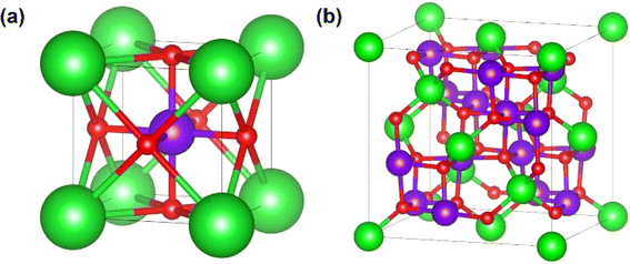

Fig. 1 Crystal structures of (a) perovskite (A – green, B – violet, O – red), (b) spinel (A – green, B – violet, O – red) oxides.

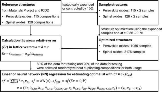
Considering the relatively large dimensionality of the feature space, the number of data points (number of structures) is small.⁵⁰ We, therefore, perform the following procedure as shown in Fig. 2: from each real structure obtained from the database called reference structure in the following, we form structures with lattice vectors isotropically expanded or contracted by 10%; these are called sample structures in the following. A 10% strain is sufficient to cover the range of possible lattice parameters of a given type of crystal structure with different chemical compositions. sf is then set to values from 0.55 to 0.75 at 0.0125 intervals and structure optimization was performed in SoftBV. The error Er – the difference between the lattice constants (defined below) following SoftBV optimization – is then collected resulting in a dataset of b_ij, R_0,ij, R_cutoff,ij, r_i, N_C, sf, and Er for each composition. In this way, the number of data points is expanded severalfold. In the case of perovskite-type oxides, SoftBV optimization does not result in any changes in fractional positions of atoms or distortions of the rectilinearity of the unit cell, and Er is defined as the mean relative error in lattice vectors a = b = c between a reference structure obtained from the database and the optimized structure by SoftBV (i.e. Er = (a_reference − a_opt)/a_reference = (b_reference − b_opt)/b_reference = (c_reference − c_opt)/c_reference). In the case of spinel-type oxides, SoftBV optimization results in small changes in the fractional positions of atoms within the unit cell. We defined the changes in fractional position per number of ions (N) as , where N is the number of atoms in the cell and Δx, Δy, and Δz are errors in fractional coordinates. Δ_site was lower than 0.01 in most of the spinel-type oxides, i.e. the error in structural parameters is mostly due to the lattice constants. Therefore, Er defined above was also used for optimizing crystal structures of the spinel-type oxides.

Fig. 2 The procedure of optimizing the screening factor.

We define a D = 11 dimensional vector of descriptors

x = (Er, R_0,AO, b_AO, N_C,AO, R_cutoff,AO, r_A, R_0,BO, b_BO, N_C,BO, R_cutoff,BO, r_B) ≡ (x₁, x₂, …, x₁₁)

and x̃ as a vector of all descriptors other than Er. The dataset of (x, sf) values for all materials and all structure expansions/contractions used for machine learning is provided in ESI.† Ionic radii (which are coordination-dependent in SoftBV) for the coordination number of 6 were used in all cases. 80% of the expanded sample data of x and sf randomly selected without duplicating compositions for training and testing were used for the training of the following regression models, and the remaining 20% for the testing. The features (x) are normalized before fitting (i.e. its average and standard deviation are set to 0 and 1, respectively).

We perform linear regressions using the “regress” function in MATLAB (version R2021a of MATLAB was used in this work):

We also perform non-linear regression using a feed-forward neural network (NN):⁵¹

sf = NN(x) (9)

The NN regressions are performed in MATLAB using “trainlm” function. Levenberg–Marquardt algorithm⁵² was used to train the NN. We considered different numbers of hidden layers and neurons. “tansig” neuron activation function is used in the following. Other neuron activation functions were tried but resulted in no improvement (not shown). The estimated optimal sf (sf_est) was obtained from eqn (8)–(10) by setting Er = 0, i.e. sf_opt = NN(0,x̃). SoftBV optimization of crystal structures with expanded or contracted lattice was carried out using sf_auto and sf_opt, and the Er was compared to evaluate the accuracy of SoftBV.

For the analysis of the relative importance of nonlinearity and coupling among the features, we use the GPR-NN method of Manzhos and Ihara.⁴⁵ The reader is referred to ref. 45, 53 and 54 for more details and context; here, we only briefly summarize the key properties of the method relevant to the purpose of the present work. The target function sf(x) is expressed as

This is a first-order additive model in (generally) redundant coordinates y = Wx, where W is the matrix of coefficients. The rows of W are defined as elements of a D-dimensional Sobol sequence⁵⁵ although other ways of setting W are possible.⁴⁵ The shapes of the functions f_n are computed using the first-order additive GPR^{53,54,56–58} in y. That is, GPR of sf(y(x)) is performed in y with an additive kernel . In this way, all functions f_n are computed simultaneously, in one linear step. The shapes of the functions f_n are optimal for given data and given W in the least squares sense.⁵⁶ The original coordinates {x_n} are also included in the set of {y_n}. If only {x_n} are included, the method defaults to first-order additive GPR.^45,56,57 The representation of eqn (10) is equivalent to a single hidden layer NN with optimal and individual to each neuron activation functions, and with weights fixed by rules rather than optimized. Matrix W is equivalent to the matrix of NN weights, while biases are subsumed in the definition of f_n. One can say that eqn (10) is an NN in x and a 1^st-order additive GPR in y. The method has the advantage that because no nonlinear optimization is done, it does not suffer from overfitting as the number of ‘neurons’ N grows beyond optimal,⁴⁵ combining the high expressive power of an NN and the robustness of linear regression (with nonlinear basis functions) which is GPR.⁵⁹

In this work, we use an additive RBF kernel in y: where . The data are normalized so that an isotropic kernel is used with a single length parameter l. In this work, we use this method to probe the importance of coupling terms by testing different N. In the limit of large N the model fully includes all coupling among features, while in the limit y = x ∈ R^D, no coupling is included. On the other hand, the construction of optimal shapes of f_n in the method is used to study the importance of nonlinearity. Similar to the case of an NN fit, sf_opt is computed from the model of eqn (10) by setting Er = 0, i.e. sf_opt = f(0,x̃).

With all methods, the loss function minimized by the regression was the SSE (sum of squared errors), , where {(x⁽ⁱ⁾, sf(x⁽ⁱ⁾))}, i = 1, …, M is the training set of size M.

3 Results and discussion

3.1 Machine learning the screening factor with linear regression and neural networks

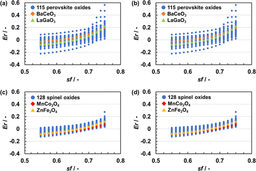
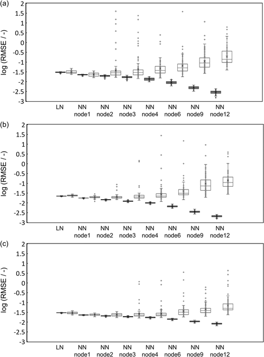
Fig. 3 shows the relationship between Er and sf. Er, namely the error in the lattice parameter, increased with an increase in sf. A larger sf makes the coulombic repulsion in BVSE stronger at long range as per eqn (1). Because the stress in a given crystal structure is to a significant degree due to coulombic repulsion, SoftBV optimization with large sf resulted in an overestimated lattice constant. The relationship between Er and sf was different for each composition but did not depend on the initial lattice parameter. For instance, for two perovskite-type oxides of BaCeO₃ (orange squares) and LaGaO₃ (green triangle), one obtains Er = 0 with sf of about 0.60 and 0.65, respectively (Fig. 3(a) and (b)). Similar results were also obtained in the case of spinel-type oxides (i.e. MnCo₂O₄ (red squares) and ZnFe₂O₄ (yellow triangles)) as shown in Fig. 3(c) and (d). These results indicate that there is only one sf minimizing Er for each material and the optimal sf is material-dependent, which suggests that an improvement can be achieved by making sf = sf(x).

Fig. 3 Error in structural parameters (Er) of (a and b) perovskite-type oxides and (c and d) spinel-type oxides following SoftBV optimization with different screening factors (sf). Figures (a) and (c) are the results of optimizing crystal structures with lattice vectors isotropically contracted by 10%. Figures (b) and (d) are the results of optimizing crystal structures with lattice vectors isotropically expanded by 10%.

The linear and single-hidden layer NN regressions of sf for perovskite- and spinel-type oxides were carried out 100 times using different combinations of training and testing data. Fig. 4 shows the distributions of root mean square error (RMSE) values of estimated sf from these regressions.

Fig. 4 Distributions of root mean square error (RMSE) of the screening factor for training (filled circles and box plots) and testing (empty circles and box plots) data obtained by linear (LN) and neural network (NN) regressions with 1 to 12 nonlinear nodes, for 100 runs with different combinations of the training and testing data for (a) perovskite-type oxides, (b) spinel-type oxides, and (c) the combined dataset.

Table 1 summarizes the maximum, minimum, and median RMSE and R² values over the 100 runs. The RMSE for the training data decreases with an increase in the number of nodes for the NN regression, as expected, while the median RMSE for the testing data was the lowest for the NN regressions with only 1–3 nodes. The results did not change when the number of the hidden layers changed to 2–12. The NN regressions with 1–3 nodes show smaller median RMSE for both training and testing data than the linear regression. Therefore, the non-linearity or coupling effects present in an NN might improve the accuracy, which is analyzed in Section 3.2, but the small number of data makes it difficult.

Table 1 Maximum, minimum, and median root mean square errors (RMSE) and R² values in the screening factor of linear and neural network (NN) regressions. “N” is the number of nodes (neurons)

Methods	RMSE/R^2 of training			RMSE/R^2 of testing
	Maximum	Minimum	Median	Maximum	Minimum	Median
Perovskite
Linear	0.032/0.83	0.025/0.73	0.031/0.75	0.049/0.89	0.024/0.56	0.03/0.76
NN, N = 1	0.024/0.90	0.019/0.84	0.023/0.86	0.036/0.93	0.016/0.71	0.024/0.85
NN, N = 2	0.023/0.95	0.014/0.86	0.02/0.89	40/0.93	0.017/0.00	0.029/0.80
NN, N = 3	0.021/0.97	0.011/0.88	0.017/0.92	24/0.95	0.014/0.00	0.029/0.79
NN, N = 4	0.018/0.97	0.010/0.91	0.014/0.95	2.5/0.94	0.015/0.01	0.036/0.71
NN, N = 6	0.013/0.99	0.006/0.95	0.009/0.98	38/0.91	0.018/0.00	0.051/0.60
NN, N = 9	0.007/1.00	0.003/0.99	0.005/0.99	12/0.85	0.026/0.00	0.088/0.34
NN, N = 12	0.004/1.00	0.002/0.99	0.003/1.00	6.2/0.76	0.040/0.00	0.14/0.17
Spinel
Linear	0.023/0.88	0.021/0.86	0.022/0.87	0.028/0.90	0.02/0.79	0.024/0.85
NN, N = 1	0.019/0.93	0.016/0.90	0.018/0.92	0.029/0.96	0.012/0.80	0.02/0.90
NN, N = 2	0.016/0.96	0.013/0.93	0.015/0.94	0.087/0.94	0.015/0.33	0.019/0.91
NN, N = 3	0.015/0.97	0.010/0.94	0.012/0.96	1.4/0.95	0.014/0.00	0.02/0.90
NN, N = 4	0.013/0.98	0.008/0.96	0.010/0.97	28/0.96	0.012/0.00	0.022/0.88
NN, N = 6	0.009/0.99	0.005/0.98	0.007/0.99	15/0.95	0.015/0.00	0.031/0.80
NN, N = 9	0.005/1.00	0.003/0.99	0.004/1.00	9.2/0.91	0.019/0.00	0.073/0.41
NN, N = 12	0.003/1.00	0.002/1.00	0.002/1.00	3.9/0.83	0.028/0.00	0.11/0.23
Perovskite + spinel
Linear	0.031/0.80	0.027/0.74	0.030/0.76	0.038/0.86	0.024/0.63	0.029/0.77
NN, N = 1	0.024/0.88	0.021/0.84	0.023/0.86	0.030/0.91	0.019/0.77	0.024/0.85
NN, N = 2	0.023/0.92	0.018/0.86	0.021/0.88	0.035/0.92	0.017/0.72	0.024/0.86
NN, N = 3	0.022/0.92	0.017/0.87	0.019/0.90	1.2/0.93	0.016/0.01	0.023/0.86
NN, N = 4	0.019/0.94	0.014/0.90	0.017/0.92	1.3/0.92	0.017/0.00	0.024/0.86
NN, N = 6	0.016/0.96	0.012/0.93	0.014/0.95	3.5/0.93	0.018/0.00	0.031/0.77
NN, N = 9	0.013/0.98	0.009/0.96	0.011/0.97	0.62/0.90	0.020/0.00	0.039/0.70
NN, N = 12	0.01/0.99	0.007/0.97	0.008/0.98	4.3/0.86	0.024/0.00	0.051/0.59

---

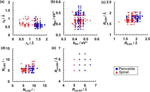
The RMSE for the testing set could be decreased, especially for the NN regression with a larger number of nodes, by increasing the number of data using both the perovskite- and spinel-type oxides data in a combined dataset. These results show that a key issue is overfitting due to the small number of data points. Fig. 5 shows the distributions of the data for selected pairs of parameters (among b_ij, R_0,ij, R_cutoff,ij, r_i, N_C). Even from two-dimensional projections that allow only a limited insight into a multivariate distribution, one can appreciate rather uneven and sparse sampling with data based on individual crystal structure types. This result indicates that the accuracy of SoftBV can be improved by estimating sf as a function of SoftBV parameters encoding composition if the space of descriptors can be adequately sampled using data for oxides of various compositions.

Fig. 5 Distributions of pairs of parameters ((a) r_A and r_B, (b) b_AO and b_BO, (c) R_0,AO and R_0,BO, (d) N_C,AO and N_C,BO, and (e) R_cut,AO and R_cut,BO) in perovskite- (blue circles) and spinel-type (red triangles) oxides data.

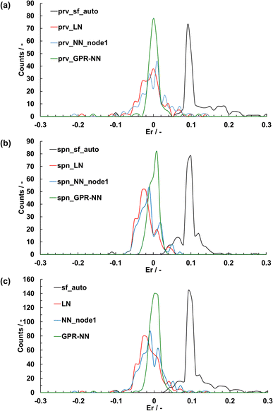
The crystal structures were optimized using each of the average sf_opt computed from each of the five linear, NN, and GPR-NN (shown in Section 3.2) regression models that had the highest R² values among the 100 runs (Fig. 6). These models used both perovskite- and spinel-type oxide data for training. The use of sf_opt improved the accuracy of structure optimization from using sf_auto. The mean absolute error (MAE) and the standard deviation (STD) of the distributions of Er are summarized in Table 2. Although an NN in principle has a higher expressive power and should be able to make a better fit, the MAE and STD for the linear model were equal or even slightly better than the NN model. This ultimately has to do with a small number of data and associated overfitting (see Fig. 4). Overall, there is no significant improvement in sf fitting quality with NN vs. linear regression, and the NN fit does not lead to an improvement in the estimation of the optimal sf and in the quality of structure optimization. While the accuracy has improved on average, the distribution of Er with the linear or NN regression is relatively broad with Er for some materials exceeding 0.1. The GPR-NN regressions (described in the following section) have the highest accuracy for optimizing the crystal structures with the narrowed distribution of Er, with MAE = 0.014 and STD = 0.025.

Fig. 6 The distribution of structure parameter errors of crystal structures optimized using automatically set screening factors in the SoftBV for each sample structure (“sf_auto”) and screening factors estimated by the linear regression (“LN”), neural network with 1 node (“NN_node1”), and the GPR-NN methods trained on the combined data set of the perovskite- and spinel-type oxides, for (a) perovskite (“prv”), (b) spinel (“spn”), and (c) both oxides.

Table 2 The mean absolute error (MAE) and the standard deviation (STD) for the error of structure optimization (that is Er defined in Methods section, dimensionless) of perovskite, spinel, and both oxides using the automatically set screening factors in the SoftBV (“Auto”) and estimated optimal screening factors by the linear, the neural network (“NN”), and the GPR-NN methods trained on the combined data set of the perovskite- and spinel-type oxides

		Auto	Linear	NN (node = 1)	GPR-NN
Perovskite oxides	MAE	0.13	0.026	0.031	0.014
	STD	0.066	0.038	0.044	0.024
Spinel oxides	MAE	0.10	0.023	0.022	0.013
	STD	0.032	0.024	0.026	0.026
Both oxides	MAE	0.12	0.025	0.026	0.014
	STD	0.053	0.032	0.036	0.025

---

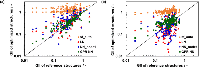
Fig. 7 shows the relationship between GII obtained from the optimized and reference structures. GII is an index for chemical stability, e.g. GII < 0.1 is typically taken to mean that the structure is stable, while GII > 0.2 is considered to be a warning that the structure may be unstable.²¹ A better GII value should be obtained when a better structure is used because the error of GII is due to the error of as eqn (7), in other words, due to the error in the distance between cations and anions. GII values of optimized structures using sf_auto are larger than those of reference structures and do not show the correlation of GII values of SoftBV-optimized structures with those of reference structures. On the other hand, there is a correlation between the GII values of structures optimized using sf_opt and the reference structures, especially for perovskite-type oxides. This result reflects the improvement of the accuracy of structure optimization with ML-estimated sf.

Fig. 7 GII of optimized and reference structures of (a) perovskite- and (b) spinel-type oxides. The crystal structures were optimized by using automatically set screening factors in the SoftBV for each sample structure (“sf_auto”) and screening factors estimated by the linear regression (“LN”), the neural network with 1 node (“NN_node1”), and the GPR-NN methods trained on the combined data set of the perovskite- and spinel-type oxides.

3.2 Analysis of the importance of nonlinearity and coupling using the GPR-NN method

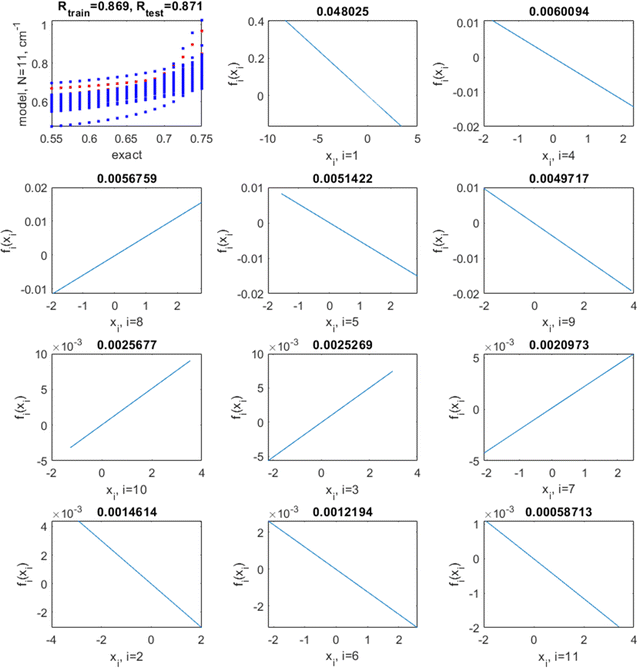
The NN results are somewhat unusual in that while there is a slight improvement in the quality of sf prediction (judged by the value of R² over the test set and the range thereof for different train-test splits) over linear regression, there is no improvement in the quality of structure optimization vs. linear regression, and the optimal NN appears to have a size of 1–3 neurons only, with the 2- or 3-neuron NN only insignificantly outperforming a 1-neuron NN, with larger NNs showing clear overfitting. NN being a universal approximator, the training set error can be made arbitrarily small, but the global quality of the model, exemplified by the test set error, is ultimately limited by the density of sampling. When sampling is sparse enough, higher-order coupling terms may not be recoverable.^54,58,60 That the sampling is sparse in this case, and that this is a limiting factor in utilizing the superior expressive power of an NN, is clear from the above comparison of fitting only the perovskite or the spinel data separately or the combined dataset.

A NN performs non-linear operations on linear combinations of inputs {x_n} introducing both nonlinearity and coupling. This is true even for a single-hidden neuron NN. We can separate these two effects with the help of the GPR-NN method. We first perform simulations where y = x, i.e. an additive model in x, . We perform a two-dimensional hyperparameters scan of the length parameter l and the GPR noise parameter σ. At each (l, σ), we perform 100 fits differing by different random splits of training and test data (whereby 20 percent of materials are used for testing and 80 for training). Note that when l becomes large (l ≫ 1 for data scaled on unit cube), kernel resolution is lost⁶¹ and the component functions f_n(x_n) become near-linear. This is illustrated in Fig. 8 for the case of l = 200, log(σ) = −3, where we show the shapes of f_n in such a limiting case as well as the correlation plots between the exact (target) values of sf and those predicted by the model for a representative run. In this case the average/min/max/standard deviation (over 100 runs) of the training set R² are 0.80/0.78/0.84/0.02, and of the test set R², 0.77/0.59/0.85/0.06, respectively, – similar to traditional linear regression. The average/min/max/standard deviation of the RMSE is 0.031/0.028/0.032/0.001 for the training and 0.032/0.028/0.039/0.002 for the test set, respectively.

Fig. 8 Top left: correlation between target (“exact”) values of the screening factor and those predicted by an additive model with a kernel length set to a large value l = 200, for training (blue) and test (red) data (some blue and red points visually overlap). The correlation coefficients between the exact and predicted values for training and testing data are also shown. The following panels show the shapes of f_i(x_i) in the order of decaying magnitude, with the magnitude (defined as var(f_i)^1/2) shown on top of each plot.

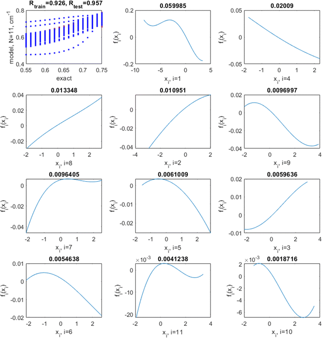
The optimal hyperparameters were chosen as those minimizing simultaneously the average test set R² and its variance (over multiple runs); they are l = 7 and log(σ) = −3. With these hyperparameters, the average/min/max/standard deviation (over 100 runs) of the training set R² are 0.89/0.88/0.92/0.01, respectively, and of the test set R², 0.85/0.71/0.93/0.05, respectively. The average/min/max/standard deviation of the RMSE is 0.022/0.019/0.023/0.001 for the training and 0.024/0.017/0.038/0.006 for the test set, respectively. This is a noticeable improvement over linear regression and the NN. This model has no coupling. The correlation plots between the exact (target) values of sf and those predicted by the model as well as the shapes of f_n in this case are shown in Fig. 9 for a representative run. They are highly nonlinear. Nonlinearity improves the quality of the model and also influences the relative importance of variables: in both the linear and the nonlinear model, the most important (by the magnitude of f_n(x_n)) variables are x₁ (Er), x₄ (R_0,AO), and x₈ (r_A). The least important is x₁₀ (N_C,AO) in the non-linear model with the optimal l = 7 while it is x₁₁ (N_C,BO) in the (practically) linear model achieved with l = 200. The order of importance of variables with small magnitudes of f_n(x_n) may differ; it is normal that the relative importance of features is different for different methods.^62,63

Fig. 9 Top left: correlation between target (“exact”) values of the screening factor and those predicted by an additive model with an optimized kernel length of l = 7, for training (blue) and test (red) data (some blue and red points visually overlap). The correlation coefficients between the exact and predicted values for training and test data are also shown. The following panels show the shapes of f_i(x_i) in the order of decaying magnitude, with the magnitude (defined as var(f_i)^1/2) shown on top of each plot.

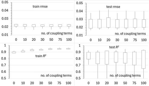
We now fix l and σ at their optimized values and test if adding coupling terms further improves the model. The results are summarized in Fig. 10. We do not observe any further improvement due to the inclusion of coupling among the features. The coupling terms are either unimportant or unrecoverable due to the low density of sampling.

Fig. 10 Statistics of training and test set errors in sf and R² values as a function of the number of coupling terms. The box shows a one-sigma interval about the mean, and the whiskers show minimum and maximum values, over 100 runs differing by random selection of training and test data.

Finally, in Fig. 6, we show the distribution of structural parameter errors achieved with the GPR-NN method (using optimal hyperparameters). The method is clearly superior over the linear regression and the NN in terms of the average error as well as the width of the error distribution, which are listed in Table 2. The optimal shapes of the nonlinear functions used with each variable, and the absence of nonlinear parameter optimization in GPR-NN allow capitalizing on the superior expressive power of a nonlinear method while retaining the robustness of linear regression.

4 Conclusions

In this study, we explored the possibility and extent of improvement of the accuracy of the SoftBV approximation by fitting the screening factor as a function of descriptors of chemical composition. We showed that it is the screening factor that can be parameterized in this way without the danger of tempering with the basis of SoftBV ideology. The features that we used are various parameters that are already available in a SoftBV calculation; that is, the screening factor as a function of those features can in principle be implemented without hardship. We first used linear and neural network models and showed, on the examples of perovskite- and spinel-type oxides which have been proposed as promising solid-state ionic conductors, that this can noticeably improve the ability of the SoftBV approximation to model structures, in particular new, putative crystal structures whose structural parameters are yet unknown.

We showed that the sampling density of the space of descriptors is an important limiting factor in the possible improvement in sf, which may even prevent one from using the superior expressive power of nonlinear models. In this work, this was palliated on one hand by combining data from different crystal structures having structural similarity (perovskite and spinel oxides in this case) and on the other hand by producing synthetic sample points from strained structures. Only a slight improvement in the screening factor regression was obtained with an NN over linear regression while no improvement over linear regression was observed in the quality of structure optimization with sf predicted by the NN model.

We then applied to this problem the recently developed GPR-NN method that allows obtaining a superior expressive power of a nonlinear approximation while avoiding nonlinear parameter optimization during regression. The method is a hybrid between an NN and kernel regression; it builds optimal shapes of nonlinear basis functions (neuron activation functions) and permits including coupling among features in a controlled way. We analyzed the relative importance of nonlinearity and coupling and found that while nonlinearity helps obtain a more accurate model, coupling terms were not important or were unrecoverable from the data. The sf predicted by GPR-NN showed the best quality of structure optimization with SoftBV and a significant improvement over linear and NN regressions.

As our tests on perovskites, spinels, and combined data show, there is a degree of portability of the machine-learned model to other crystal structures with similar coordination environments of ions. The models are in principle not portable to crystal structures with significantly different coordination environments simply because other parts of the feature vector x, which are environment-dependent SoftBV parameters, will be different and unsampled. While this is a limitation, there is still much value in exploring different compositions of particular crystal symmetries, of which there is typically a finite number of interest in particular applications.

Data availability

A list of all crystal structures with their database identifiers as well as the dataset used in machine learning are available in ESI.† The GPR-NN code is available in ref. 45.

Author contributions

Keisuke Kameda: data curation, software, visualization, investigation, formal analysis, writing – original draft preparation, writing – reviewing and editing. Takaaki Ariga: data curation, software, visualization, investigation, formal analysis. Kazuma Ito: data curation, software, formal analysis. Manabu Ihara: supervision, project administration, funding acquisition, resources, writing – reviewing and editing. Sergei Manzhos: conceptualization, methodology, supervision, resources, project administration, writing – original draft preparation, writing – reviewing and editing.

Conflicts of interest

We declare that we have no conflict of interest.

Acknowledgements

This work was supported by JST-Mirai Program, Japan, Grant Number JPMJMI22H1. We thank Prof. Stefan Adams of National University of Singapore for discussions and consultations. We thank Digital Research Alliance of Canada on whose computers some of the calculations were performed.

References

1. J. E. Saal, S. Kirklin, M. Aykol, B. Meredig and C. Wolverton, JOM, 2013, 65, 1501–1509.
2. B. Liu, J. Zhao, Y. Liu, J. Xi, Q. Li, H. Xiang and Y. Zhou, J. Mater. Sci. Technol., 2021, 88, 143–157.
3. P. Priya and N. R. Aluru, npj Comput. Mater., 2021, 7, 1–12.
4. Z. Wang, Z. Sun, H. Yin, X. Liu, J. Wang, H. Zhao, C. H. Pang, T. Wu, S. Li, Z. Yin and X.-F. Yu, Adv. Mater., 2022, 34, 2104113.
5. S. Manzhos and M. Ihara, Physchem, 2022, 2, 72–95.
6. Q. Liang, S. Wang, Y. Yao, P. Dong and H. Song, Adv. Funct. Mater., 2023, 33, 2300825.
7. M. D. Allendorf, Z. Hulvey, T. Gennett, A. Ahmed, T. Autrey, J. Camp, E. S. Cho, H. Furukawa, M. Haranczyk, M. Head-Gordon, S. Jeong, A. Karkamkar, D.-J. Liu, J. R. Long, K. R. Meihaus, I. H. Nayyar, R. Nazarov, D. J. Siegel, V. Stavila, J. J. Urban, S. P. Veccham and B. C. Wood, Energy Environ. Sci., 2018, 11, 2784–2812.
8. J. Hwang, R. R. Rao, L. Giordano, Y. Katayama, Y. Yu and Y. Shao-Horn, Science, 2017, 358, 751–756.
9. Q. Wang, L. Velasco, B. Breitung and V. Presser, Adv. Energy Mater., 2021, 11, 2102355.
10. K. Alberi, M. B. Nardelli, A. Zakutayev, L. Mitas, S. Curtarolo, A. Jain, M. Fornari, N. Marzari, I. Takeuchi, M. L. Green, M. Kanatzidis, M. F. Toney, S. Butenko, B. Meredig, S. Lany, U. Kattner, A. Davydov, E. S. Toberer, V. Stevanovic, A. Walsh, N.-G. Park, A. Aspuru-Guzik, D. P. Tabor, J. Nelson, J. Murphy, A. Setlur, J. Gregoire, H. Li, R. Xiao, A. Ludwig, L. W. Martin, A. M. Rappe, S.-H. Wei and J. Perkins, J. Phys. D: Appl. Phys., 2018, 52, 013001.
11. H. Xu, Y. Yu, Z. Wang and G. Shao, Energy Environ. Mater., 2019, 2, 234–250.
12. W. Chen, Y. Li, D. Feng, C. Lv, H. Li, S. Zhou, Q. Jiang, J. Yang, Z. Gao, Y. He and J. Luo, J. Power Sources, 2023, 561, 232720.
13. A. B. Muñoz-García, A. M. Ritzmann, M. Pavone, J. A. Keith and E. A. Carter, Acc. Chem. Res., 2014, 47, 3340–3348.
14. M. Coduri, M. Karlsson and L. Malavasi, J. Mater. Chem. A, 2022, 10, 5082–5110.
15. R. Li, R. Deng, Z. Wang, Y. Wang, G. Huang, J. Wang and F. Pan, J. Solid State Electrochem., 2024, 28, 317.
16. J. Lee, T. Lee, K. Char, K. J. Kim and J. W. Choi, Acc. Chem. Res., 2021, 54, 3390–3402.
17. Q. Ma and F. Tietz, ChemElectroChem, 2020, 7, 2693–2713.
18. P. Hohenberg and W. Kohn, Phys. Rev., 1964, 136, B864–B871.
19. W. Kohn and L. J. Sham, Phys. Rev., 1965, 140, A1133–A1138.
20. L. L. Wong, K. C. Phuah, R. Dai, H. Chen, W. S. Chew and S. Adams, Chem. Mater., 2021, 33, 625–641.
21. H. Chen, L. L. Wong and S. Adams, Acta Crystallogr., Sect. B: Struct. Sci., Cryst. Eng. Mater., 2019, 75, 18–33.
22. H. Chen and S. Adams, IUCrJ, 2017, 4, 614–625.
23. I. D. Brown, Chem. Rev., 2009, 109, 6858–6919.
24. R. G. Parr and R. G. Pearson, J. Am. Chem. Soc., 1983, 105, 7512–7516.
25. S. Adams, in Bond Valences, ed. I. D. Brown and K. R. Poeppelmeier, Springer, Berlin, Heidelberg, 2014, pp. 91–128.
26. S. Adams and R. P. Rao, Phys. Chem. Chem. Phys., 2009, 11, 3210–3216.
27. A. K. Rappe, C. J. Casewit, K. S. Colwell, W. A. I. Goddard and W. M. Skiff, J. Am. Chem. Soc., 1992, 114, 10024–10035.
28. W. H. Zachariasen, J. Less-Common Met., 1978, 62, 1–7.
29. R. D. Shannon, Acta Crystallogr., Sect. A: Cryst. Phys., Diffr., Theor. Gen. Crystallogr., 1976, 32, 751–767.
30. R. D. Shannon and C. T. Prewitt, Acta Crystallogr., Sect. B: Struct. Crystallogr. Cryst. Chem., 1969, 25, 925–946.
31. M. M. Obeid, J. Liu, Y. Shen and Q. Sun, Chem. Mater., 2023, 35, 3256–3264.
32. K. M. Rießbeck, M. Seibald, S. Schwarzmüller, D. Baumann and H. Huppertz, Eur. J. Inorg. Chem., 2023, 26, e202300304.
33. Z. Deng, D. Chen, M. Ou, Y. Zhang, J. Xu, D. Ni, Z. Ji, J. Han, Y. Sun, S. Li, C. Ouyang and Z. Wang, Adv. Energy Mater., 2023, 13, 2300695.
34. Y.-C. Yin, J.-T. Yang, J.-D. Luo, G.-X. Lu, Z. Huang, J.-P. Wang, P. Li, F. Li, Y.-C. Wu, T. Tian, Y.-F. Meng, H.-S. Mo, Y.-H. Song, J.-N. Yang, L.-Z. Feng, T. Ma, W. Wen, K. Gong, L.-J. Wang, H.-X. Ju, Y. Xiao, Z. Li, X. Tao and H.-B. Yao, Nature, 2023, 616, 77–83.
35. P. Naskar, S. Mondal, B. Biswas, S. Laha and A. Banerjee, Sustainable Energy Fuels, 2023, 7, 4189–4201.
36. Y. Okada, T. Kimura, K. Motohashi, A. Sakuda and A. Hayashi, Electrochemistry, 2023, 91, 077009.
37. Y. Nishitani, S. Adams, K. Ichikawa and T. Tsujita, Solid State Ionics, 2018, 315, 111–115.
38. Y. A. Morkhova, M. Rothenberger, T. Leisegang, S. Adams, V. A. Blatov and A. A. Kabanov, J. Phys. Chem. C, 2021, 125, 17590–17599.
39. Y. Pu, R. Dai and S. Adams, Phys. Status Solidi A, 2021, 218, 2100318.
40. R. J. Morelock, Z. J. L. Bare and C. B. Musgrave, J. Chem. Theory Comput., 2022, 18, 3257–3267.
41. J. Richter, P. Holtappels, T. Graule, T. Nakamura and L. J. Gauckler, Monatsh. Chem., 2009, 140, 985–999.
42. K. Karuppiah and A. M. Ashok, Nanomater. Energy, 2019, 8, 51–58.
43. X. Li and M. Ihara, J. Electrochem. Soc., 2015, 162, F927.
44. A. Manthiram, Nat. Commun., 2020, 11, 1550.
45. S. Manzhos and M. Ihara, J. Phys. Chem. A, 2023, 127, 7823–7835.
46. A. Jain, S. P. Ong, G. Hautier, W. Chen, W. D. Richards, S. Dacek, S. Cholia, D. Gunter, D. Skinner, G. Ceder and K. A. Persson, APL Mater., 2013, 1, 011002.
47. S. Gates-Rector and T. Blanton, Powder Diffr., 2019, 34, 352–360.
48. P. Giannozzi, S. Baroni, N. Bonini, M. Calandra, R. Car, C. Cavazzoni, D. Ceresoli, G. L. Chiarotti, M. Cococcioni, I. Dabo, A. D. Corso, S. de Gironcoli, S. Fabris, G. Fratesi, R. Gebauer, U. Gerstmann, C. Gougoussis, A. Kokalj, M. Lazzeri, L. Martin-Samos, N. Marzari, F. Mauri, R. Mazzarello, S. Paolini, A. Pasquarello, L. Paulatto, C. Sbraccia, S. Scandolo, G. Sclauzero, A. P. Seitsonen, A. Smogunov, P. Umari and R. M. Wentzcovitch, J. Phys.: Condens. Matter, 2009, 21, 395502.
49. J. P. Perdew, K. Burke and M. Ernzerhof, Phys. Rev. Lett., 1996, 77, 3865–3868.
50. S. Manzhos, S. Tsuda and M. Ihara, Phys. Chem. Chem. Phys., 2023, 25, 1546–1555.
51. G. Montavon, G. B. Orr and K.-R. Mueller, Neural Networks: Tricks of the Trade, Springer, Berlin Heidelberg, 2nd edn, 2012.
52. W. H. Press, B. P. Flannery, S. A. Teukolsky and W. T. Vetterling, Numerical Recipes in C: The Art of Scientific Computing, Cambridge University Press, Cambridge ; New York, 2nd edn, 1992.
53. S. Manzhos and M. Ihara, Artif. Intell. Chem., 2023, 1, 100013.
54. S. Manzhos, T. Carrington and M. Ihara, Artif. Intell. Chem., 2023, 1, 100008.
55. I. M. Sobol’, USSR Comput. Math. Math. Phys., 1967, 7, 86–112.
56. S. Manzhos, E. Sasaki and M. Ihara, Mach. Learn.: Sci. Technol., 2022, 3, 01LT02.
57. O. Ren, M. A. Boussaidi, D. Voytsekhovsky, M. Ihara and S. Manzhos, Comput. Phys. Commun., 2022, 271, 108220.
58. M. A. Boussaidi, O. Ren, D. Voytsekhovsky and S. Manzhos, J. Phys. Chem. A, 2020, 124, 7598–7607.
59. C. M. Bishop, Pattern Recognition and Machine Learning, Springer, Singapore, 2006.
60. S. Manzhos and T. Carrington, J. Chem. Phys., 2006, 125, 084109.
61. S. Manzhos and M. Ihara, J. Chem. Phys., 2024, 160, 021101.
62. M. Nukunudompanich, H. Yoon, L. Hyojae, K. Kameda, M. Ihara and S. Manzhos, MRS Adv., 2024, 9, 857–862.
63. J. Im, S. Lee, T.-W. Ko, H. W. Kim, Y. Hyon and H. Chang, npj Comput. Mater., 2019, 5, 1–8.

---

Footnote

† Electronic supplementary information (ESI) available: The list of structures used in this work together with their respective database identifiers, as well as the dataset used for machine learning. See DOI: https://doi.org/10.1039/d4dd00152d

---