Transfer learning based on atomic feature extraction for the prediction of experimental ¹³C chemical shifts

Abstract

Forecasting experimental chemical shifts of organic compounds is a long-standing challenge in organic chemistry. Recent advances in machine learning (ML) have led to routines that surpass the accuracy of ab initio Density Functional Theory (DFT) in estimating experimental ¹³C shifts. The extraction of knowledge from other models, known as transfer learning, has demonstrated remarkable improvements, particularly in scenarios with limited data availability. However, the extent to which transfer learning improves predictive accuracy in low-data regimes for experimental chemical shift predictions remains unexplored. This study indicates that atomic features derived from a message passing neural network (MPNN) forcefield are robust descriptors for atomic properties. A dense network utilizing these descriptors to predict ¹³C shifts achieves a mean absolute error (MAE) of 1.68 ppm. When these features are used as node labels in a simple graph neural network (GNN), the model attains a better MAE of 1.34 ppm. On the other hand, embeddings from a self-supervised pre-trained 3D aware transformer are not sufficiently descriptive for a feedforward model but show reasonable accuracy within the GNN framework, achieving an MAE of 1.51 ppm. Under low-data conditions, all transfer-learned models show a significant improvement in predictive accuracy compared to existing literature models, regardless of the sampling strategy used to select from the pool of unlabeled examples. We demonstrated that extracting atomic features from models trained on large and diverse datasets is an effective transfer learning strategy for predicting NMR chemical shifts, achieving results on par with existing literature models. This method provides several benefits, such as reduced training times, simpler models with fewer trainable parameters, and strong performance in low-data scenarios, without the need for costly ab initio data of the target property. This technique can be applied to other chemical tasks opening many new potential applications where the amount of data is a limiting factor.

---

Introduction

NMR chemical shifts

NMR chemical shifts are valuable in the structure elucidation of organic compounds within classical and computer-assisted frameworks.^1–5 Carbon chemical shifts have been used to elucidate reaction products,⁶ metabolites,⁷ and natural products, including in the revision of the structures.^8–10 Furthermore, chemical shifts carry information about the local chemical environments of atoms and have been used as descriptors for predicting chemical reactivity^11,12 and in QSAR/QSPR models.¹³ Prediction of carbon chemical shifts from the molecular structure has been extensively studied and many methods have been developed, ranging from ab initio to fully data-driven methods.^14,15

Predicting carbon NMR shifts from molecular structures from the first principles is computationally intensive. Typical prediction of NMR using ab initio methods involves geometry optimization followed by single-point calculation including specific NMR calculation. Obtaining accurate geometry in the geometry optimization process is the usual bottleneck, as it involves multiple single-point calculations. In addition to errors from the electronic structure calculations, treatment of solvation, conformational flexibility, and rovibronic effects introduce further errors.¹⁶ Considering all these factors comprehensively is computationally impractical at any level of theory that ensures reasonable accuracy. For example, even a basic DFT calculation of chemical shifts on an inexpensive geometry is too resource-intensive for large-scale rapid structure elucidation. The chosen functional, basis set, and solvation model influences the precision of DFT predictions for NMR shifts.¹⁷ Although different results in the literature are reported on different sets for the same computational protocols, the best-reported protocol achieves a root mean square error (RMSE) of 3.68 ppm when compared to experimental shifts.¹⁷ This is insufficient for typical applications, as an initial investigation has shown that an accuracy of 1.1-1.2 ppm of MAE is necessary for correctly identifying 99% of molecules in the metabolomic database.¹⁸

The errors of DFT-predicted shifts have a systematic component that can be corrected using available experimental data. Lodewyk et al.¹⁶ developed a linear scaling protocol for different combinations of levels of theory, solvents, and solvation models, and their findings were compiled in the CHESHIRE repository.¹⁹ This became the standard for chemical shift prediction using DFT. Gao et al.²⁰ went beyond linear interpolation and constructed a deep neural network that takes molecular structure and descriptors derived from calculated DFT shielding constants as input to predict experimental chemical shifts. Their method demonstrated superior performance, achieving an RMSE of 2.10 ppm, which is a significant notable improvement over the 4.77 ppm RMSE the authors report from linear regression on the same small test set.

The Exp5K dataset, developed as part of the CASCADE project,¹² is the largest dataset that compares empirically scaled DFT chemical shifts with experimental shifts. The authors excluded structures where DFT significantly disagreed with experimental results to avoid introducing noise from potential misassignments in the experimental data. This exclusion inevitably removes challenging examples where the disagreement arises from DFT's inability to accurately predict shifts due to molecular complexity. Additionally, the atom ordering was altered when comparing DFT with experimental shifts, leading to the unjustified exclusion of some examples from the dataset. After correcting the atom order, the calculated shifts deviate from the experiments with an MAE of 2.21 ppm and an RMSE of 3.31 ppm.† This should be considered the most realistic measure of the accuracy of DFT-calculated shifts corrected with linear scaling. These correction methods, along with others reported in the literature,^21,22 enhance the accuracy of predictions but do not reduce their computational cost.

On the other hand, data-driven methods are significantly faster by several orders of magnitude. The efficiency of machine learning in predicting carbon chemical shifts arises from the avoidance of expensive geometry optimizations or electronic structure computations. Nevertheless, the top models in the literature explicitly include geometrical data of the lowest energy conformers in their predictions.^12,23–25 The compromise is achieved by utilizing inexpensive forcefield geometries instead of costly DFT-optimized geometries.

The accuracy of predictions in data-driven models is influenced by the quality and quantity of the training data.^26,27 By using experimental data for training, common errors in ab initio methods can be avoided. The most extensive open NMR shift database with fully assigned spectra is nmrshiftdb2.²⁸ User-contributed databases like this often face issues such as missing solvent and temperature details, peak misassignments, measurement noise, and incorrect structure identification. A model's performance is limited not only by the quantity but also by the quality of data. Thus, models that perform well in low-data scenarios are necessary when data is scarce and when prioritizing high-quality data over quantity.

Transfer learning

Transfer learning involves using a model trained on one task as a foundation for training on another task, known as a downstream task.²⁹ Generally, pre-training is performed on a similar task with a much larger dataset, followed by training on a smaller dataset for the specific task of interest. Feature extraction and fine-tuning are two main implementations of transfer learning.‡ The choice of method depends on task similarity, the size and architecture of the pre-trained model, and the amount of available data. Feature extraction is commonly used in computer vision,^30,31 while fine-tuning is widely used in language models.^32,33

One of the major challenges for machine learning in chemistry is the scarcity of training data.^34,35 Acquiring experimental and high-quality ab initio data is costly, and more affordable ab initio data often comes with substantial errors. Complex models, which are generally necessary to represent intricate chemical phenomena, demand a large amount of data for training. Integrating chemical and physical knowledge and intuition into the model architecture is one strategy to lessen the required training data.³⁶ Transfer learning provides an alternative method to enhance models and can be used alongside other techniques to address issues related to limited data for chemical problems.

Most previous studies employ transfer learning for chemical models by initially training models on data generated from ab initio methods and then fine-tuning them on experimental data.^12,37,38 This quasi-transfer approach is effective if a significantly larger amount of ab initio data compared to the available experimental data can be produced. However, certain experimental properties like the smell, catalytic activity, and reaction yield are difficult or impossible to model using ab initio methods, while calculating others such as NMR properties, free energies, and absorption spectra can be prohibitively costly. In such cases, pre-training must be conducted on less relevant tasks where it is feasible to generate large-scale datasets.

Related work

In the notable CASCADE study,¹² graph neural networks (GNN) were employed to predict experimental chemical shifts. The ExpNN-ff model takes 3D structures optimized using MMFF forcefield as the way to incorporate geometrical information while maintaining relatively low computational cost. The authors implemented an interesting double-transfer learning training. First, the model was trained on DFT-optimized geometries and scaled DFT shifts. Second, the model was retrained on DFT-optimized geometries and experimental shifts, keeping the interaction layers frozen. Finally, the model was retrained again on forcefield geometries and experimental shifts, keeping the readout layers frozen. It is unclear what advantage this approach has over doing single-step transfer learning, updating all layers in the model simultaneously. Still, the ExpNN-ff model with an MAE of 1.43 ppm on a 500 hold-out test set performs better than the DFT with empirical scaling which has an MAE of 2.21 ppm on the whole training dataset of around 5000 compounds.

To avoid the costly DFT calculations for large molecules during the generation of the pre-training dataset, Han and Choi³⁷ pretrained a GNN using the QM9 dataset of DFT shielding constants. They subsequently fine-tuned the model using an experimental chemical shifts database that includes larger molecules and atoms such as P, Cl, and S, which are absent in the QM9 dataset. The authors evaluated the model in low data scenarios, achieving an MAE of approximately 2.3 ppm with 2112 training examples. Nonetheless, the authors pre-trained on ab initio NMR data on a dataset comparable to the size of the experimental dataset used to fine-tune the model, similar to the approach used in CASCADE.

The first example of adopting true transfer learning for predicting chemical shifts was done in a recent work by El Samman et al.³⁹ The authors extracted atomic embeddings from the last interaction layer from the SchNet model⁴⁰ trained to predict molecular energies on the QM9 dataset. The authors tested linear and feedforward network models for different chemical tasks, including predicting carbon chemical shifts calculated by HOSE codes.⁴¹ However, the dataset for the chemical shifts consisted of only 200 examples of shifts predicted by the HOSE code, so the performance relative to the literature models trained from scratch could not be assessed.

To tackle low-data scenarios without resorting to transfer learning, Rull et al.⁴² modified a GNN architecture to enhance its efficiency in such conditions. While the modified architecture performed better in low-data scenarios than a similar GNN model, it significantly underperformed in high-data scenarios. This underscores the importance of considering the volume of training data when evaluating model performance and designing model architectures.

The most recent advance in transfer learning for carbon chemical shifts comes from Shiota et al.⁴³ The authors explored descriptors derived from neural network forcefield and employed them in kernel ridge regression (KRR). They show this is a viable strategy and achieve robust results. However, their work focuses on predicting computed shifts using the classical KRR algorithm. In this work, we focus on FFN and GNN downstream models and compare two different types of pre-trained models with particular emphasis on low-data regimes. We prove that using more complex downstream models, such as GNN, can be beneficial.

Approach

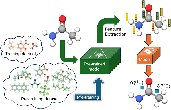
In an ideal situation, pre-training is performed on a highly similar task for which either more data is available or it is significantly cheaper to generate. However, such tasks are rarely available for any downstream chemical task, necessitating some form of compromise. Many of the latest pre-trained chemical models employ self-supervised pre-training tasks on huge unlabeled datasets of 2D chemical structures.^44–47 Conversely, there are numerous instances of quasi-transfer learning, involving pre-training on datasets of ab initio calculated properties of the size comparable to the available experimental datasets.^12,37 We propose the atomic feature extraction from the models pre-trained for different chemical tasks on larger datasets, and we evaluate it by predicting experimental ¹³C chemical shifts. The proposed approach is illustrated in Fig. 1.

Fig. 1 Transfer learning based on atomic feature extraction.

Choice of pre-training task and model

The downstream task in this study is to predict the chemical shifts of carbon atoms. Predicting other atomic properties influenced by the chemical environment of the atom is the most relevant task. However, no other atomic properties have as extensive experimental data as chemical shifts. Fortunately, many models designed for predicting molecular properties incorporate atomic representations within their architectures.^48,49 Moreover, the pre-trained model must consider geometrical information since chemical shifts are influenced by molecular conformation. Therefore, most pre-trained models based on 2D molecular structures are not suitable candidates. This leads us to neural network forcefields, whose architectures are designed to sum atomic energy contributions.§ We selected the MACE-OFF23 transferable organic forcefield,^50,51 which is state-of-the-art for predicting DFT molecular energies, open-source, and trained on a reasonably large dataset. Since we are not concerned with inference time, we chose the large variant of the forcefield. The other model we tested is Uni-Mol,⁵² a 3D-aware self-supervised pre-trained transformer known for its performance in downstream molecular property prediction tasks. Although self-supervised pre-training is less directly related to atomic property prediction, it is done on an even larger dataset. The model includes atomic representation in its architecture, and integrates geometrical information in its embeddings, making it appropriate for this transfer learning approach. Both models are pre-trained on datasets significantly larger than the available NMR datasets, which is one of the requirements we propose for this transfer learning approach. There is a certain overlap between structures present in the NMR dataset and the pre-training dataset, however, there are also many examples of structures in the NMR dataset not present in the pre-training datasets.

Feature extraction

We extract atomic embeddings from the first of two interaction layers in the large variant of the MACE-OFF23 forcefield. This approach contrasts with the method of El Samman et al.,³⁹ where embeddings are extracted from the final interaction layer of the SchNet model.⁴⁰ This decision was motivated by the difference between tasks. The embeddings from initial layers should be more general and therefore more transferable to tasks that significantly differ from pre-training tasks. We retain only the invariant portion of the embedding to ensure rotational and translational invariance, resulting in a 244-dimensional vector atomic embedding. Given that Uni-Mol is intended as a backbone pre-trained model for various downstream tasks, we directly extract the atomic representation from the output of the backbone, yielding a 512-dimensional vector per atom, invariant to translation and rotation. Both models use atomic coordinates and identities as inputs, akin to the input used by typical ab initio codes, and produce atomic embeddings for each atom as outputs.

Models architecture

We evaluated two distinct types of downstream models: a feedforward network (FFN) and a graph neural network (GNN). For the FFN, we assume that the pre-trained model has captured all necessary information regarding the chemical environment of each carbon atom. We use the embeddings of carbon atoms as input and train the network to predict chemical shifts. Additionally, we tested the GNN based on the GraphSAGE⁵³ architecture, which facilitates the exchange of information between different atomic environment embeddings. This leads to a more robust model as it can learn more relevant embeddings for NMR shifts. Our decision to use the GraphSAGE architecture was based on a brief initial study examining the effectiveness of well-known message-passing architectures applied to chemical problems in the literature.

Unlike the other methods where fully connected graphs with a cutoff distance or graphs with implicitly represented hydrogens have been used, we used a chemical graph where all atoms are explicitly included. Consequently, GNN models require atomic connectivity as input, whereas FFN models only need atomic coordinates. Finally, after the message passing layers, the atomic embeddings of carbon atoms are fed into a readout feedforward network to predict chemical shifts. Both methodologies are illustrated in Fig. 2. The ensemble of two models, implemented as taking the average between the predictions of each model is also tested.

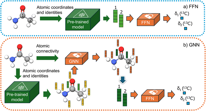Fig. 2 (a) FNN model (b) GNN model. Only orange models are trained, while the green models' weights are frozen.

Low-data regime

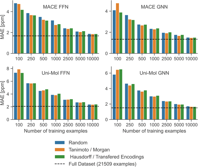
To evaluate model performance with fewer training examples, we selected varying quantities of samples from the original dataset, treating it as a pool of unlabeled examples. Although this dataset is smaller than the typical molecular datasets of unlabeled molecules, it is sufficiently large to compare different sampling methods. We examined three sampling strategies: random sampling, MaxMin sampling⁵⁴ based on the Tanimoto distance⁵⁵ between Morgan fingerprints,⁵⁶ and MaxMin sampling based on the undirected Hausdorff distance⁵⁷ between sets of transferred embeddings of all carbon atoms in two molecules. The directed Hausdorff distance between two sets of vectors A and B is defined as:
where d(a, b) is any distance metric between two vectors. However, the directed Hausdorff distance is not symmetric, so we use the undirected Hausdorff distance, employing the Euclidean distance as the distance metric d:

In our scenario, sets of vectors represent sets of transferred embeddings of carbon atoms. While we could have used embeddings of all atoms, the carbon atom embeddings also convey information about their neighboring atoms. Since our primary interest lies in the differences in carbon atom environments between two molecules, we used only the embeddings of carbon atoms, which also reduces the computational cost, a crucial factor when sampling large pools of examples.

Results

The mean absolute error (MAE), root mean square error (RMSE), and Pearson correlation coefficient (ρ) between true and predicted shifts for all models are presented in Table 1. The results are based on a modified test set, where we excluded a couple of broken examples from the original test set. Additional details, including more performance metrics for each model and examples of molecules where models fail, can be found in ESI.† The ensemble of two independently trained GNN models performs the best, with the lowest MAE and RMSE. MACE models outperform their Uni-Mol equivalents significantly, indicating that the forcefield is an excellent option for the pre-training task. Even though the Uni-Mol GNN has a lower MAE than the MACE FFN model, its RMSE is higher, highlighting the necessity to report at least both MAE and RMSE when reporting the model's performance. Regarding parameter efficiency, MACE GNN is by far the best model.

Table 1 Performance on a test set and number of trainable parameters

Model	MAE [ppm]	RMSE [ppm]	ρ	N parameters
MACE FFN	1.68	2.74	0.9986	1.3 × 10^6
Uni-Mol FFN	2.07	3.40	0.9978	1.8 × 10^6
Ensemble MACE & Uni-Mol FFN	1.65	2.68	0.9986	3.1 × 10^6
MACE GNN	1.34	2.38	0.9989	1.9 × 10^6
Uni-Mol GNN	1.51	2.81	0.9985	9.3 × 10^6
Ensemble MACE & Uni-Mol GNN	1.28	2.37	0.9989	1.0 × 10^7

---

A comparison with relevant literature models that take forcefield geometries as input is shown in Fig. 3. The ensemble of two GNNs and MACE GNN performs equally well as the best-reported literature models. Comparison with models trained using the same train/test split is more reliable, and the FullSSPrUCe model is trained on the larger portion of the nmrshiftdb2 database, which explains its slightly better performance. In any case, since all reported models are solvent agnostic, it is clear that the accuracy has reached its limit because it is not unusual for ¹³C shifts to differ by more than 1 ppm in different solvents.

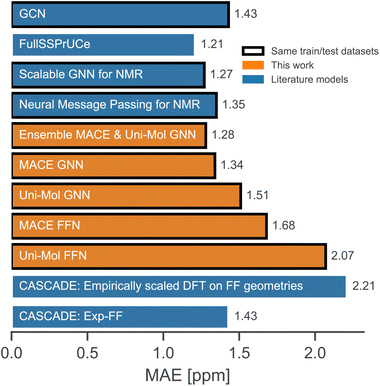Fig. 3 Comparison with the literature models.^{12,23–25,58}

The distinct advantages of our models are their simpler architectures† and fewer trainable parameters, which result in significantly reduced training time. We do not consider the parameters of pre-trained models because the entire training dataset can be encoded by pre-trained models before training, making the training time independent of the number of parameters of the pre-trained model. However, the complexity of pre-trained models affects inference speed. Fortunately, the bottleneck in inference is conformer generation, so our models are faster to train and equally fast for inference.

Low-data regimes

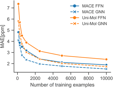
To simulate low-data regimes, we sampled data points from the training dataset, maintaining the same model architectures† as used in the full data scenario to emphasize the effectiveness of transfer learning. Nonetheless, the performance can be enhanced by optimizing hyperparameters for low-data regimes, especially by reducing model complexity and the dropout rate. Furthermore, an additional molecule was excluded from the test set because MACE-based models gave erroneous predictions for that molecule.†

Fig. 4 illustrates that the performance of all models is improved with an increased number of training examples. Notably, the MACE models outperform Uni-Mol models in extremely low-data scenarios, regardless of the downstream model architecture. This highlights the choice of pre-training task and model architecture as the main influence on performance in low-data regimes. Fig. 5 compares models in this paper with a model that performs similarly on the full dataset (2019 Model), a model specifically designed for low-data scenarios (2023 Model), and a classical HOSE Code model.^41,42 Transfer learning significantly boosts accuracy in low-data scenarios compared to models trained from scratch. Furthermore, there is no trade-off between performance in high-data and low-data scenarios, unlike in the 2019 model.⁴²

Fig. 4 Performance of our models in low-data regimes simulated using random sampling.

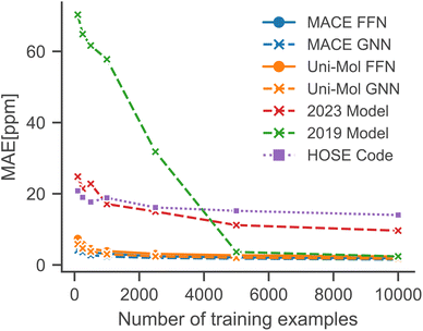Fig. 5 Comparison with literature models in low-data regimes simulated using random sampling.^41,42

Tautomer identification

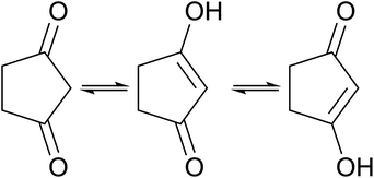
In contrast to other outliers that possess uncommon functional groups or complex bonding and geometrical configurations,† one simple molecule yielded unsatisfactory results across all models developed in this study. Detailed examination reveals that the structure listed in the dataset, 1,3-cyclopentanedione, does not correspond to the tautomer present in solution under the conditions where the experimental chemical shifts were obtained. The tautomeric equilibrium that takes place for this molecule is illustrated in Fig. 7.

Fig. 6 The effect of three different sampling strategies.

Fig. 7 Different tautomers of 1,3-cyclopentanedione (a, b, and c).

Experimental findings on a similar compound⁵⁹ indicate that the two tautomers on the right-hand side of Fig. 7 predominate in solution, with rapid interconversion between them on the NMR time scale. Consequently, the NMR chemical shift of this compound represents an average of the chemical shifts of these two structures. The predicted shifts by the Ensemble MACE & Unimol GNN model for the diketo form (structure a) and the averaged prediction for the keto–enol forms (structures b and c) are illustrated in Fig. 8. The comparison of structure a, structure b, and the averaged prediction for structures b and c with observed shifts is shown in Table 2. The good match with experiment when using the prediction for the mixture of tautomers b and c is consistent with the rapid interconversion between two tautomeric structures, and demonstrates the ability of the model to assist in typical organic chemistry problems.

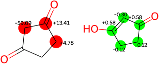Fig. 8 Errors [ppm] in predictions by ensemble GNN model in structure a (left) and structures b and c (right).

Table 2 Mean absolute errors of shifts predicted by the Ensemble GNN model

	Structure a	Structure b	Structures b and c
MAE [ppm]	19.03	3.42	0.34

---

Conclusion

We introduced atomic feature extraction as a transfer learning method applicable to both atomic and molecular-level prediction tasks. Unlike previous quasi-transfer methods, this approach does not require generating ab initio data for the target property. Moreover, the only information needed are atomic coordinates and atomic connectivity.

We evaluated this method on the prediction of experimental ¹³C chemical shifts, a well-studied atomic property prediction task. Our method performs on par with the best models trained from scratch and surpasses them in low-data scenarios. When using this transfer learning approach, we demonstrated that the details of the sampling strategy used to select from the pool of unlabeled examples don't matter (Fig. 6). Lastly, we identified the MPNN forcefield as a superior candidate for pre-trained models for transfer learning compared to self-supervised pre-trained models.

The proven efficacy in low-data scenarios reveals new potential uses for this transfer learning approach in chemical problems with limited experimental data and in tasks where plenty of data exists but predictions are limited by data quality. For chemical shifts, employing more precise geometries and data with recorded solvents and peaks assigned through multiple spectra will enhance the accuracy of data-driven models. This enhancement is feasible only if models can be trained on less data, which can be achieved through the transfer learning method described here.

Methods

Data

The dataset utilized in this work is taken from Kwon et al.,²⁵ and is derived from the original dataset published by Jonas and Kuhn.⁵⁸ It includes a predefined train/test split. This dataset comprises molecules with experimental spectra from nmrshiftdb2, which contain elements H, C, O, N, P, S, and F, and have no more than 64 atoms. The molecular geometries are obtained as the lowest energy conformers found in EDTKG conformer search⁶⁰ followed by MMFF minimization.⁶¹ Molecules that failed rdkit sanitization, likely due to version discrepancies, were excluded. A detailed summary of the resulting dataset is available in the ESI.†

Models

FFN models consist of simple fully connected layers with exponential linear unit (ELU) activation functions.⁶² The final layer is linear without any activation function. GNN models employ GraphSAGE message passing layers with ELU activation function, followed by a readout feedforward network of the same type as FFN models. Dropout was applied after each layer in all models.⁶³ The models were trained using L1 loss (mean absolute error) as the cost function and the AdamW optimizer with a weight decay of 0.01.⁶⁴ Hyperparameters were optimized through automated hyperparameter tuning and manual adjustments. Additional training and model architecture details can be found in the ESI.†

Computational details

We accessed the pre-trained models using code from the associated repositories. Rdkit^65,66 (version 2023.09.5) was employed to process data, extract atomic connectivity from molecular structures, and perform MaxMin sampling. PyTorch⁶⁷ (version 2.2.1) and PyTorch Lightning⁶⁸ (version 2.2.1) were used for constructing and training FFN models, while PyTorch Geometric⁶⁹ (version 2.5.2) was used for GNN models. All models were trained on a single Nvidia L4 Tensor core GPU. MaxMin sampling and Morgan fingerprints with a radius of 3 were implemented using rdkit. The Hausdorff distance was calculated using the scipy package.^70,71 Training for low-data examples continued until the validation loss ceased to decrease or until 800 epochs were reached. We sampled 120% of training data points for each regime, then randomly divided the data into train and validation sets. This ensured that the validation dataset size was always 20% of the training dataset size, and the train/validation split was performed as usual, making the conditions closer to a real low-data regime. Conversely, testing was conducted on the entire test set for a realistic performance evaluation. Note that this approach differs from the work we compared low-data performance to, where the test set size was proportional to the training dataset size.

Code and data availability

The code used in the paper is publicly available in the repository https://github.com/zarkoivkovicc/AFE-TL-for-13C-NMR-chemical-shifts under the ASL license, including the transfer learned models' weights. Pre-trained models and original datasets can be downloaded from the code repositories of the corresponding publications.

Author contributions

Ž. I.: conceptualization, investigation, methodology, software, visualization, writing – original draft J. J.: funding acquisition, supervision, writing – review and editing J. H.: resources, supervision, writing – review and editing.

Conflicts of interest

There are no conflicts to declare.

Acknowledgements

Ž. I. acknowledge the IQTC-UB Master grant. J. J. acknowledges Maria de Maeztu grant (code: CEX2021-001202-M). Z. I. acknowledges recepit of an European Commision Erasmus+ Scholarship Grant from the TCCM Masters.

References

1. J. Stothers, Carbon-13 NMR Spectroscopy: Organic Chemistry, A Series of Monographs, Elsevier, 2012, vol. 24.
2. U. Sternberg, R. Witter and A. S. Ulrich, Annual Reports on NMR Spectroscopy, Academic Press, 2004, vol. 52, pp. 53–104.
3. A. Bagno and G. Saielli, Theor. Chem. Acc., 2007, 117, 603–619.
4. A. Wu, Q. Ye, X. Zhuang, Q. Chen, J. Zhang, J. Wu and X. Xu, Precis. Chem., 2023, 1, 57–68.
5. Z. Huang, M. S. Chen, C. P. Woroch, T. E. Markland and M. W. Kanan, Chem. Sci., 2021, 12, 15329–15338.
6. T. D. Michels, M. S. Dowling and C. D. Vanderwal, Angew. Chem., Int. Ed., 2012, 51, 7572–7576.
7. M. DiBello, A. R. Healy, H. Nikolayevskiy, Z. Xu and S. B. Herzon, Acc. Chem. Res., 2023, 56, 1656–1668.
8. S. D. Rychnovsky, Org. Lett., 2006, 8, 2895–2898.
9. H. A. Sánchez-Martínez, J. A. Morán-Pinzón, E. del Olmo Fernández, D. L. Eguiluz, J. F. Adserias Vistué, J. L. López-Pérez and E. G. De León, J. Nat. Prod., 2023, 86, 2294–2303.
10. D. J. Tantillo, Nat. Prod. Rep., 2013, 30, 1079–1086.
11. C. P. Gordon, C. Raynaud, R. A. Andersen, C. Copéret and O. Eisenstein, Acc. Chem. Res., 2019, 52, 2278–2289.
12. Y. Guan, S. V. Shree Sowndarya, L. C. Gallegos, P. C. St. John and R. S. Paton, Chem. Sci., 2021, 12, 12012–12026.
13. R. P. Verma and C. Hansch, Chem. Rev., 2011, 111, 2865–2899.
14. E. Jonas, S. Kuhn and N. Schlörer, Magn. Reson. Chem., 2022, 60, 1021–1031.
15. I. Cortés, C. Cuadrado, A. Hernández Daranas and A. M. Sarotti, Front. Nat. Prod., 2023, 2, 1122426.
16. M. W. Lodewyk, M. R. Siebert and D. J. Tantillo, Chem. Rev., 2012, 112, 1839–1862.
17. E. Benassi, J. Comput. Chem., 2017, 38, 87–92.
18. Y. Yesiltepe, N. Govind, T. O. Metz and R. S. Renslow, J. Cheminf., 2022, 14, 64.
19. T. Cheshire, P. Ramblenm, D. J. Tantillo, M. R. Siebert and M. W. Lodewyk, CHEmical SHift REpository with Coupling Constants Added Too, http://cheshirenmr.info/.
20. P. Gao, J. Zhang, Q. Peng, J. Zhang and V.-A. Glezakou, J. Chem. Inf. Model., 2020, 60, 3746–3754.
21. A. M. Sarotti and S. C. Pellegrinet, J. Org. Chem., 2009, 74, 7254–7260.
22. D. Xin, C. A. Sader, O. Chaudhary, P.-J. Jones, K. Wagner, C. S. Tautermann, Z. Yang, C. A. Busacca, R. A. Saraceno, K. R. Fandrick, N. C. Gonnella, K. Horspool, G. Hansen and C. H. Senanayake, J. Org. Chem., 2017, 82, 5135–5145.
23. J. Williams and E. Jonas, Chem. Sci., 2023, 14, 10902–10913.
24. J. Han, H. Kang, S. Kang, Y. Kwon, D. Lee and Y.-S. Choi, Phys. Chem. Chem. Phys., 2022, 24, 26870–26878.
25. Y. Kwon, D. Lee, Y.-S. Choi, M. Kang and S. Kang, J. Chem. Inf. Model., 2020, 60, 2024–2030.
26. L. Budach, M. Feuerpfeil, N. Ihde, A. Nathansen, N. Noack, H. Patzlaff, F. Naumann and H. Harmouch, The Effects of Data Quality on Machine Learning Performance, arXiv, 2022, preprint, arXiv:2207.14529,  DOI:10.48550/arXiv.2207.14529.
27. F. J. Fan and Y. Shi, Bioorg. Med. Chem., 2022, 72, 117003.
28. S. Kuhn and N. E. Schlörer, Magn. Reson. Chem., 2015, 53, 582–589.
29. A. Farahani, B. Pourshojae, K. Rasheed and H. R. Arabnia, A Concise Review of Transfer Learning, arXiv, 2021, preprint, arXiv:2104.02144,  DOI:10.48550/arXiv.2104.02144.
30. G. Kumar and P. K. Bhatia, 2014 Fourth International Conference on Advanced Computing & Communication Technologies, Rohtak, India, 2014, pp. 5–12.
31. E. d. S. Puls, M. V. Todescato and J. L. Carbonera, An Evaluation of Pre-Trained Models for Feature Extraction in Image Classification, arXiv, 2023, preprint, arXiv:2310.02037,  DOI:10.48550/arXiv.2310.02037.
32. T. B. Brown, B. Mann, N. Ryder, M. Subbiah, J. Kaplan, P. Dhariwal, A. Neelakantan, P. Shyam, G. Sastry, A. Askell, S. Agarwal, A. Herbert-Voss, G. Krueger, T. Henighan, R. Child, A. Ramesh, D. M. Ziegler, J. Wu, C. Winter, C. Hesse, M. Chen, E. Sigler, M. Litwin, S. Gray, B. Chess, J. Clark, C. Berner, S. McCandlish, A. Radford, I. Sutskever and D. Amodei, Language Models Are Few-Shot Learners, arXiv, 2020, preprint, arXiv:2005.14165,  DOI:10.48550/arXiv.2005.14165.
33. B. Weng, Navigating the Landscape of Large Language Models: A Comprehensive Review and Analysis of Paradigms and Fine-Tuning Strategies, arXiv, 2024, preprint, arXiv:2404.09022,  DOI:10.48550/arXiv.2404.09022.
34. D. van Tilborg, H. Brinkmann, E. Criscuolo, L. Rossen, R. Özçelik and F. Grisoni, Curr. Opin. Struct. Biol., 2024, 86, 102818.
35. S. G. Espley, E. H. E. Farrar, D. Buttar, S. Tomasi and M. N. Grayson, Digital Discovery, 2023, 2, 941–951.
36. G. E. Karniadakis, I. G. Kevrekidis, L. Lu, P. Perdikaris, S. Wang and L. Yang, Nat. Rev. Phys., 2021, 3, 422–440.
37. H. Han and S. Choi, J. Phys. Chem. Lett., 2021, 12, 3662–3668.
38. F. H. Vermeire and W. H. Green, Chem. Eng. J., 2021, 418, 129307.
39. A. El-Samman, S. De Castro, B. Morton and S. De Baerdemacker, Can. J. Chem., 2024, 102, 275–288.
40. K. Schütt, P.-J. Kindermans, H. E. Sauceda Felix, S. Chmiela, A. Tkatchenko and K.-R. Müller, Adv. Neural Inf. Process. Syst., 2017, 991–1001.
41. W. Bremser, Anal. Chim. Acta, 1978, 103, 355–365.
42. H. Rull, M. Fischer and S. Kuhn, J. Cheminf., 2023, 15, 114.
43. T. Shiota, K. Ishihara and W. Mizukami, Digital Discovery, 2024, 1714.
44. W. Ahmad, E. Simon, S. Chithrananda, G. Grand and B. Ramsundar, ChemBERTa-2: Towards Chemical Foundation Models, arXiv, 2022, preprint, arXiv:2209.01712,  DOI:10.48550/arXiv.2209.01712.
45. J. Ross, B. Belgodere, V. Chenthamarakshan, I. Padhi, Y. Mroueh and P. Das, Large-Scale Chemical Language Representations Capture Molecular Structure and Properties, arXiv, 2022, preprint, arXiv:2106.09553,  DOI:10.48550/arXiv.2106.09553.
46. J. Xia, Y. Zhu, Y. Du and S. Z. Li, A Systematic Survey of Chemical Pre-trained Models, arXiv, 2022, preprint, arXiv:2210.16484,  DOI:10.48550/arXiv.2210.16484.
47. Y. Rong, Y. Bian, T. Xu, W. Xie, Y. Wei, W. Huang and J. Huang, Self-Supervised Graph Transformer on Large-Scale Molecular Data, arXiv, 2020, preprint, arXiv:2007.02835,  DOI:10.48550/arXiv.2007.02835.
48. E. Heid, K. P. Greenman, Y. Chung, S.-C. Li, D. E. Graff, F. H. Vermeire, H. Wu, W. H. Green and C. J. McGill, J. Chem. Inf. Model., 2024, 64, 9–17.
49. J. Gilmer, S. S. Schoenholz, P. F. Riley, O. Vinyals and G. E. Dahl, Neural Message Passing for Quantum Chemistry, arXiv, 2017, preprint, arXiv:1704.01212,  DOI:10.48550/arXiv.1704.01212.
50. D. P. Kovács, J. H. Moore, N. J. Browning, I. Batatia, J. T. Horton, V. Kapil, W. C. Witt, I.-B. Magdău, D. J. Cole and G. Csányi, MACE-OFF23: Transferable Machine Learning Force Fields for Organic Molecules, arXiv, 2023, preprint, arXiv:2312.15211,  DOI:10.48550/arXiv.2312.15211.
51. I. Batatia, S. Batzner, D. P. Kovács, A. Musaelian, G. N. C. Simm, R. Drautz, C. Ortner, B. Kozinsky and G. Csányi, The Design Space of E(3)-Equivariant Atom-Centered Interatomic Potentials, arXiv, 2022, preprint, arXiv:2205.06643,  DOI:10.48550/arXiv.2205.06643.
52. G. Zhou, Z. Gao, Q. Ding, H. Zheng, H. Xu, Z. Wei, L. Zhang and G. Ke, Uni-Mol: A Universal 3D Molecular Representation Learning Framework, ChemRxiv, 2023, preprint,  DOI:10.26434/chemrxiv-2022-jjm0j-v4.
53. W. L. Hamilton, R. Ying and J. Leskovec, Inductive Representation Learning on Large Graphs, arXiv, 2017, preprint, arXiv:1706.02216,  DOI:10.48550/arXiv.1706.02216.
54. M. Ashton, J. Barnard, F. Casset, M. Charlton, G. Downs, D. Gorse, J. Holliday, R. Lahana and P. Willett, Quantitative Structure-Activity Relationships, 2002, vol. 21, 598–604.
55. D. Bajusz, A. Rácz and K. Héberger, J. Cheminf., 2015, 7, 20.
56. D. Rogers and M. Hahn, J. Chem. Inf. Model., 2010, 50, 742–754.
57. T. Birsan and D. Tiba, System Modeling and Optimization, Kluwer Academic Publishers, Boston, 2006, vol. 199, pp. 35–39.
58. E. Jonas and S. Kuhn, J. Cheminf., 2019, 11, 50.
59. V. Lacerda, M. G. Constantino, G. V. J. da Silva, Á. C. Neto and C. F. Tormena, J. Mol. Struct., 2007, 828, 54–58.
60. S. Riniker and G. A. Landrum, J. Chem. Inf. Model., 2015, 55, 2562–2574.
61. T. A. Halgren, J. Comput. Chem., 1996, 17, 490–519.
62. D.-A. Clevert, T. Unterthiner and S. Hochreiter, Fast and Accurate Deep Network Learning by Exponential Linear Units (ELUs), arXiv, 2015, preprint, arXiv:1511.07289,  DOI:10.48550/arXiv.1511.07289.
63. N. Srivastava, G. Hinton, A. Krizhevsky, I. Sutskever and R. Salakhutdinov, J. Mach. Learn. Res., 2014, 15, 1929–1958.
64. I. Loshchilov and F. Hutter, Decoupled Weight Decay Regularization, arXiv, 2017, preprint, arXiv:1711.05101,  DOI:10.48550/arXiv.1711.05101.
65. RDKit.
66. G. Landrum, P. Tosco, B. Kelley, Ric, D. Cosgrove, Sriniker, R. Vianello, Gedeck, N. Schneider, G. Jones, E. Kawashima, D. Nealschneider, A. Dalke, B. Cole, M. Swain, S. Turk, A. Savelev, A. Vaucher, M. Wójcikowski, I. Take, V. F. Scalfani, D. Probst, K. Ujihara, G. Godin, A. Pahl, R. Walker, J. Lehtivarjo and F. Berenger, strets123 and jasondbiggs, Rdkit/Rdkit: Release_2023.09.5, Zenodo, 2024.
67. A. Paszke, S. Gross, F. Massa, A. Lerer, J. Bradbury, G. Chanan, T. Killeen, Z. Lin, N. Gimelshein, L. Antiga, A. Desmaison, A. Köpf, E. Yang, Z. DeVito, M. Raison, A. Tejani, S. Chilamkurthy, B. Steiner, L. Fang, J. Bai and S. Chintala, PyTorch: An Imperative Style, High-Performance Deep Learning Library, arXiv, 2019, preprint, arXiv:1912.01703,  DOI:10.48550/arXiv.1912.01703.
68. W. Falcon, The PyTorch Lightning team, PyTorch Lightning, arXiv, 2019, preprint, https://github.com/Lightning-AI/pytorch-lightning/blob/bfa8b7be2d99b980afa62f5cb0433326bcfd2ef0/CITATION.cff#L1.
69. M. Fey and J. E. Lenssen, Fast Graph Representation Learning with PyTorch Geometric, arXiv, 2019, preprint, arXiv:1903.02428,  DOI:10.48550/arXiv.1903.02428.
70. P. Virtanen, R. Gommers, T. E. Oliphant, M. Haberland, T. Reddy, D. Cournapeau, E. Burovski, P. Peterson, W. Weckesser, J. Bright, S. J. Van Der Walt, M. Brett, J. Wilson, K. J. Millman, N. Mayorov, A. R. J. Nelson, E. Jones, R. Kern, E. Larson, C. J. Carey, İ. Polat, Y. Feng, E. W. Moore, J. VanderPlas, D. Laxalde, J. Perktold, R. Cimrman, I. Henriksen, E. A. Quintero, C. R. Harris, A. M. Archibald, A. H. Ribeiro, F. Pedregosa, P. Van Mulbregt, S. Py 1. 0 Contributors, A. Vijaykumar, A. P. Bardelli, A. Rothberg, A. Hilboll, A. Kloeckner, A. Scopatz, A. Lee, A. Rokem, C. N. Woods, C. Fulton, C. Masson, C. Häggström, C. Fitzgerald, D. A. Nicholson, D. R. Hagen, D. V. Pasechnik, E. Olivetti, E. Martin, E. Wieser, F. Silva, F. Lenders, F. Wilhelm, G. Young, G. A. Price, G.-L. Ingold, G. E. Allen, G. R. Lee, H. Audren, I. Probst, J. P. Dietrich, J. Silterra, J. T. Webber, J. Slavič, J. Nothman, J. Buchner, J. Kulick, J. L. Schönberger, J. V. De Miranda Cardoso, J. Reimer, J. Harrington, J. L. C. Rodríguez, J. Nunez-Iglesias, J. Kuczynski, K. Tritz, M. Thoma, M. Newville, M. Kümmerer, M. Bolingbroke, M. Tartre, M. Pak, N. J. Smith, N. Nowaczyk, N. Shebanov, O. Pavlyk, P. A. Brodtkorb, P. Lee, R. T. McGibbon, R. Feldbauer, S. Lewis, S. Tygier, S. Sievert, S. Vigna, S. Peterson, S. More, T. Pudlik, T. Oshima, T. J. Pingel, T. P. Robitaille, T. Spura, T. R. Jones, T. Cera, T. Leslie, T. Zito, T. Krauss, U. Upadhyay, Y. O. Halchenko and Y. Vázquez-Baeza, Nat. Methods, 2020, 17, 261–272.
71. A. A. Taha and A. Hanbury, IEEE Trans. Pattern Anal. Mach. Intell., 2015, 37, 2153–2163.

---

Footnotes

† Electronic supplementary information (ESI) available. See DOI: https://doi.org/10.1039/d4dd00168k

‡ In the literature, the term fine-tuning is not well-defined; it can refer to the second phase of training in general or to training models with weights initialized from other models. Here, we refer to the latter and simply call the second phase of training ‘training,’ as opposed to the ‘pre-training’ in the first phase.

§ This architecture design is not mandatory. The only requirement for architecture is the presence of atomic embeddings within the model.

---