A prediction model for CO₂/CO adsorption performance on binary alloys based on machine learning

Abstract

Despite the rapid development of computational methods, including density functional theory (DFT), predicting the performance of a catalytic material merely based on its atomic arrangements remains challenging. Although quantum mechanics-based methods can model ‘real’ materials with dopants, grain boundaries, and interfaces with acceptable accuracy, the high demand for computational resources no longer meets the needs of modern scientific research. On the other hand, Machine Learning (ML) method can accelerate the screening of alloy-based catalytic materials. In this study, an ML model was developed to predict the CO₂ and CO adsorption affinity on single-atom doped binary alloys based on the thermochemical properties of component metals. By using a greedy algorithm, the best combination of features was determined, and the ML model was trained and verified based on a data set containing 78 alloys on which the adsorption energy values of CO₂ and CO were calculated from DFT. Comparison between predicted and DFT calculated adsorption energy values suggests that the extreme gradient boosting (XGBoost) algorithm has excellent generalization performance, and the R-squared (R²) for CO₂ and CO adsorption energy prediction are 0.96 and 0.91, respectively. The errors of predicted adsorption energy are 0.138 eV and 0.075 eV for CO₂ and CO, respectively. This model can be expected to advance our understanding of structure–property relationships at the fundamental level and be used in large-scale screening of alloy-based catalysts.

---

1 introduction

CO₂ Reduction Reaction (CO₂RR) refers to the rapid conversion of CO₂ into various high-value-added chemical products, such as methane, methanol, formic acid, and syngas, using suitable catalysts and specific technical means.¹ It holds tremendous potential in addressing the aggravating greenhouse effect.^2–4 In addition, the extraction of fossil fuels has endangered the ecological balance in some areas. Also, coal mining has claimed the lives of many miners.⁵ For these reasons, in recent years, various countries have been paying increasing attention to renewable energy, including solar, wind, geothermal, and biomass, to diversify the sources of energy and reduce dependence on a single energy carrier. Metal materials, especially transition metals, are the most widely used catalysts for CO₂RR due to their excellent electrical conductivity and catalytic activity.⁶ However, numerous studies have indicated that single-metal catalysts exhibit drawbacks such as high reduction overpotential, low selectivity toward desired products, susceptibility to deactivation, and high cost.⁷ Therefore, seeking catalytic materials for efficient catalytic reduction of CO₂ is meaningful. Binary alloys, for instance, which span a vast set of materials and have shown attractive promise for catalyzing many reactions and the potential to substitute the noble metal catalysts^8–10 and are frequently used as conventional catalysts, which possess enhanced catalytic performance and improved cycling stability in CO₂RR.¹¹

Compared with the traditional experimental “trial and error method,” theoretical methods such as density functional theory (DFT) calculations have apparent advantages in their ability to rapidly screen materials. Nevertheless, predictions of adsorption energy on bimetallic surfaces are challenging due to the exponentially large possibility of alloy compositions, which makes the computational screening too time- and resource-consuming even for methods like DFT.^12–15 To this end, developing adsorption predictive models, for example, based on machine learning (ML), is necessary to rapidly survey appropriate adsorption energies for reactions of interest.¹⁶ Although there are theoretical models for predicting the chemisorption energy of adsorbates on pure metal surfaces, for example, the d-band center model estimates the adsorbate-metal interactions based on the coupling of d-states of metal with adsorbates,^17,18 generalizing these simplified thermochemical models to bimetallic materials is unpractical, which will be shown in this study.

In recent years, ML methods have emerged as a powerful approach for screening promising catalyst materials.^19,20 Among all the popular ML methods, decision trees, multilayer perceptron, extreme gradient boosting, and support vector regression have emerged as the most well-known supervised learning approach for data mining. They can use existing data to find regularity and map the correlation between the varieties of properties with desired prediction targets.²¹ Moreover, they can handle many irrelevant inputs because they incorporate internal feature selection as an integral part of the algorithm. Furthermore, ensemble learning can significantly improve the prediction accuracy of decision trees by aggregating multiple weak learners.^22,23

A series of studies have been carried out utilizing ML to predict adsorption energy on the surface of materials.^24–27 Shi et al. investigated ML modeling of CO adsorption energy on surface-layered alloys doped with 23 metals including Cr, Mn, and Fe, and screened out CO₂RR catalysts based on suitable CO adsorption energy range (−1.68 to −1.64 eV), in their layered alloy model, five layers (2 × 2) of surface cells are used to simulate the surface of the alloy, each consisting of only one metal, and the bottom three layers are always composed of the same elements, changing only the doping of the first layer, which consists of 20% or 40% of the doping atoms.²⁸ Liu investigated the adsorption energies on binary alloy surfaces of Pd_nAu_16−n alloyed surface with different Pd content (n = 1–16) by ML prediction and concluded that the isolated Pd top sites surrounded by Au atoms are stable adsorption sites.²⁹ Nayak et al. predicted adsorption energies of H, O, N, OH, NO, and CO on fcc(111) surface top sites of 25 different transition metals including Ir, Pt, and Au with an average root-mean-square error (RMSE) of about 0.4 eV by random forest regression.³⁰ Prediction of adsorption energies on metal and alloy surfaces was also reported using the XGBoost regression,³¹ artificial neural network algorithm,^32,33 random forest,³⁴ and other methods.^35,36 However, the feature selection method, which can quickly select the most suitable features for prediction from dozens or even hundreds of machine learning features, was seldom used in previous studies. Moreover, ML models aiming to predict adsorption energies on alloys often focus on binary alloys with only layered structures, i.e. the entire topmost layer of the metal was replaced by another metal element, while the actual configuration of alloys in real catalysts could be much more complex.²⁹

In this study, we directly exploit the adsorption energies of CO₂ and CO on surfaces of a wide range of binary alloys using ML methods without any assumptions of linearity, i.e. we do not assume the adsorption energy on alloys to be a linear combination of adsorption affinity on its two component metal surfaces.³⁵ We have chosen a feature selection method called the greedy algorithm,³⁷ which traverses all combinations of features and finally locates the optimal combination. From these, we select the best feature combinations to be used in the subsequent algorithms for prediction. The results show that the algorithm with XGBoost works best. As an extension to previous literature,²⁹ in this study, we focus on single-atom doped binary alloys rather than alloys with layered structures. We admit that this is still a significantly simplified model for realist materials, but the ML method and models that are developed and shown to be valid in this study can be further extended for alloys with more complex structures. This approach can be used to rapidly predict adsorption energies with high accuracy. The root-mean-square error (RMSE) for the entire dataset is 0.075 eV and 0.138 eV for the adsorption energy of CO and CO₂, respectively, which are comparable to the accuracy of Batchelor's ML models for predicting *OH and *O adsorption energies,³⁸ except that this study covers a much wider range of materials. This model goes beyond the traditional strategies and can be used to facilitate the discovery of novel alloy catalytic materials.

2 Methods

2.1. Quantum mechanics calculations

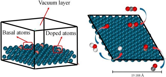
All DFT calculations were performed using the Vienna ab initio simulation package (VASP 5.4.4)³⁹ with the generalized gradient approximation (GGA-PBE)⁴⁰ functional. The cutoff energy of the plane-wave basis set was set to 400 eV. We used Monkhorst–Pack k-point samplings of 2 × 2 × 1.⁴¹ The atomic positions were relaxed until the force on all flexible atoms and total energy changes were no more than 1 × 10⁻² eV Å⁻¹ and 1 × 10⁻⁶ eV, respectively. As explained in Section 1, in this study we focus on alloys with a single dopant atom on the surface (Fig. 1). It should be noted that, as our material system is periodic, the doping ratio is 1 dopant atom for every 16 metal atoms on a (4 × 4) material surface. The bottom two layers remained fixed at truncated optimized bulk positions corresponding to substrate metals while other layers and CO₂/CO/H/O adsorbate underwent complete relaxation. It is important to note that by using a thicker slab model, for example, four layers of metal with the top two layers fully relaxed, the calculated adsorption energy values could be more accurate. However, we assumed that the errors of using the three-layer model are small compared to the accuracy of the ML model itself and prioritized low computational cost over precision in the slab model choice. A vacuum space of 20 Å was inserted to eliminate interactions between neighboring slabs. The available choices for adsorption sites are top, bridge, and hollow. However, we have only calculated the adsorption energies on the top sites and used them to train the ML model. There are two reasons for this choice. Firstly, we assessed the impact of adsorption sites on the adsorption energy of CO₂ and CO on Cu/Cr alloy (ESI Fig. S1†) and found that the most stable adsorption sites are always the on-top sites. Secondly, requiring adsorption energies on all possible sites would significantly increase the burden on users of this ML model. Although it cannot be guaranteed that top sites are always the most stable sites for all adsorbates on all materials, from the perspective of a predictive ML model, using the adsorption energies only on top sites as inputs is a good tradeoff between accuracy and usability.

Fig. 1 Schematic diagram of the calculation model.

2.2. Machine learning models

Four ML regression algorithms were implemented in the Python language using Scikit-learn⁴² and Pytorch⁴³ libraries. Outlines of these four algorithms are sketched below. Since these methods are well-established and widely used, implementation details can be found in the corresponding references.

(i) Multi-layer perceptron (MLP³²) is called a feedforward neural network, the basis of a deep neural network. It can optimize the objective function and improve the model accuracy. The hyperparameters that need to be optimized are the learning rate (L_r), dropout (D_t), L₂ regular term (L₂), number of hidden layer (N_l), number of hidden layer neurons (N_n), and activation function.⁴⁴ Commonly used activation functions include the Sigmoid function,⁴⁵ Tanh function,⁴⁶ and ReLU function,⁴⁷ etc. A visual depiction of the MLP model's diagram is shown in Fig. 2a. If only one layer is included, this model is called a wide single-layer linear model and can be expressed as

y = W^T_wide{x,∅(x)} + b (1)

In this case, the parameters of the model are represented by W and b; the raw data entered are represented by x; linear layers of neural networks by the kernel function are designated as ∅(x).

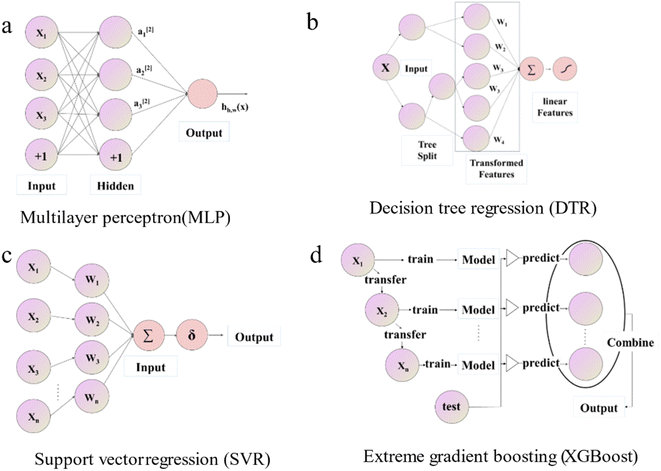Fig. 2 Schematic diagram of the structure of different machine learning algorithms for (a) MLP, (b) DTR, (c) SVR, and (d) XGBoost.

In cases where there is more than one layer, it is referred to as a multi-layer neural network (MLP), and can be defined as

a^l+1 = f(W^l_deepa^l + b^l) (2)

where ‘l’ represents the l-th layer; f() represents the activation function; Wand b^l are weight and bias parameters.

(ii) Decision Tree Regression (DTR⁴⁸) shown in Fig. 2b is an ML algorithm for predicting continuous numerical values. Its details are specified by hyperparameters including max_depth (D_m), min_samples_leaf (S_l), and min_samples_split (S_s). It can be described mathematically by

where h_m represents the m-th base learner; β_m the coefficient of the h_m base learner; a_m the parameters of the h_mbase learner; x the raw data entered, and M the number of base learners.

(iii) Support Vector Regression (SVR⁴⁹) demonstrated in Fig. 2c is a typical optimization problem; its mathematical model is a convex quadratic programming model, which can be used for pattern classification, regression estimation, and density estimation problems. SVR regressor aims to find a unique linear model f(x) = w × x + b to approximate. The tunable model hyperparameters are kernel type (kernel), penalty factor (C), and precision (epsilon).

(iv) Extreme gradient boost (XGBoost⁵⁰) illustrated in Fig. 2d is an ensemble learning model with high efficiency, flexibility, and lightness. Assume that we are currently in the m-th iteration, Ø is the defined loss function, the optimization step can be represented by the minimization of eqn (4).

2.3. Feature selection procedure

As a fundamental assumption, we assume that the adsorption affinity of adsorbates on an alloy is related to the physicochemical properties of the component elements of the alloy. Specifically, we considered 12 physicochemical properties of the component elements of an alloy as listed in Table 1. Property values of all metal elements involved in this study were obtained from the Nuclear Energy Agency (NEA) thermochemical database.⁵¹

Table 1 List of physicochemical properties of component elements of an alloy that are to be used to construct the features of an alloy. Their code names in our model are also provided

Physicochemical property	Code name
Atomic number	AN
Electronegativity	EN
First ionization energy	FE
Density	G
Period of the element	PN
Radius	R
Specific heat capacity	C
IUPAC group number	GN
First electron affinity	AE
Gas phase standard entropy of formation	S
Gas phase standard enthalpy of formation	H
Gas phase standard gibbs free energy of formation	G

---

Contrary to previous studies, the values of these 12 properties were not directly used in ML trainings.⁵² On the other hand, we defined ML features in a more general way. Here we define a ‘feature’ to be a numerical value associated with an alloy material that can be used as an input to the ML model. Features of an alloy are constructed from the properties listed in Table 1 in the following way. Since we considered binary alloys, there are 12 property values for each element and 24 property values in total, giving the first 24 features. Then we performed arithmetic operations (addition, subtraction, multiplication, and division) on each feature of two elements, given 48 (12 × 4) additional features. Finally, we included the DFT-calculated adsorption energy of O and H on the alloy surface, bringing the final number of features to 74 for each alloy material. A complete list of these features and their code names in our model is listed in ESI Table S1.†

Contrary to intuition, an excessive number of features will result in reduced training efficiency of machine learning and adversely affect prediction accuracy.⁵³ This means not all 74 features defined in ESI Table S1† are equally important for the ML model. To find which feature or which combination of features is most effective in predicting the adsorption affinity of alloys, a greedy algorithm (Fig. 3a) was utilized and described below.^54,55

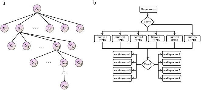Fig. 3 Schematic diagram of optimization algorithm flow, (a) the greedy algorithm of feature screening, (b) acceleration algorithm utilizing parallel computing.

Initially, a simple linear regression was used to predict the correlation between the DFT adsorption energy values and a single feature, and the feature with the lowest RMSE value out of the 74 total features was selected as the optimal one. Secondly, one of the remaining 73 features was selected so that the prediction based on the two features-tuple can produce the smallest RSME. This process was repeated iteratively until all possible feature combinations were tested, resulting in optimal features combinations.⁵⁶ For example, in Fig. 3a the combination of features X1, X3, X73, X72, … was found to be the best.

This feature selection process is also accelerated using multi-process concurrency, GPU acceleration, and multi-server operation methods, as shown in Fig. 3b. Initially, code 1 calls all servers simultaneously, and then code 2 is commanded on the active server for multi-process optimization, thus achieving accelerated optimization. It is worth noting that the GPU version shows a more pronounced acceleration effect. Generally, in any chemometrics-based approach, the performance of the techniques is evaluated using different indices related to the simulated and actual values. The current work explored the use of three various statistical error measures, namely, Mean absolute error (MAE), Root Mean Square Error (RMSE), and R-squared (R²),^57,58 coupled with one fitness indices including the Pearson correlation coefficient (P) (as shown in equation). Before the simulation stage, an external validation process based on k-1 fold (the 78 sets of alloys data are divided into 77 training sets and 1 test set, and all the combined prediction learning is cycled, and finally, the individual prediction results of 78 data are output) cross-validation was conducted to optimize the models' performance, increase the model integrity, and minimize errors.

The Pearson correlation coefficient (P) is primarily used to examine the correlation between feature values and parameters.

R-squared (R²) represents the degree to which a regression line fits the observed data points.

Root Mean Square Error (RMSE) indicates the extent of the differences between predicted values and actual values.

Mean Absolute Percentage Error (MAE) represents the average of the absolute errors between predicted and observed values, expressed as a percentage.

where y^t_i and y^p_i represent the actual and predicted values, and denote any two feature values.

3 Results and discussion

3.1. DFT calculation results

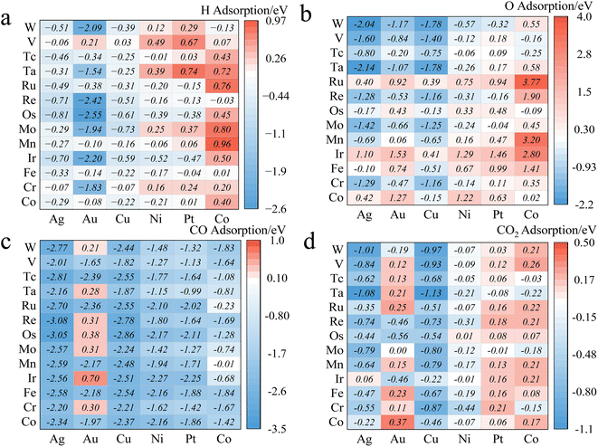
We constructed three-layer slabs with (4 × 4) surface unit cells for all alloys. One atom on the surface layer of the slab was replaced by another metal atom to create a single-atom doped binary alloy. Specifically, we considered 78 alloys for CO₂/CO/H/O adsorption energies (Fig. 4 and ESI Table S2†). Base elements of the alloys (components M1) include Cu, Ni, Ag, Au, Pt, and Co, and the doped single-atoms (M2) include Co, Cr, Fe, Ir, Mn, Mo, Os, Re, Ru, Ta, Tc, V, W. We considered the effect of increasing the thickness of the slab to four layers but found that (ESI Fig. S2†) the difference in adsorption energy values is around 0.08 eV at least on the Cu/Co and Pd/Co materials, which falls well below the accuracy threshold of machine learning prediction. This observation can be corroborated by Tomacruz et al., who showed that three layers of metal atoms are enough to describe a surface.²⁵ In addition, we have partially investigated aspects such as two-layer atom doping effects on the adsorption site (ESI Fig. S3†). Results demonstrated an error margin lower than 0.09 eV. In all cases, as explained in Section 2.1, only the top sites are considered. Adsorption energy (E_ads) is defined as E_ads(M) = E[M*] − E[M(g)] − E[*], where M* represents adsorbed M and * refers to an empty site. According to this definition, more negative E_ads means stronger adsorption.

Fig. 4 DFT-calculated adsorption energy of (a) H, (b) O, (c) CO, and (d) CO₂ on 78 single-atom doped binary alloys. The x-axis represents the basal elements (M1), and the y-axis shows the doped elements (M2) of the alloys. Numbers are visualized by colors where red and blue represent weak (larger E_ads) and strong (smaller E_ads) adsorption, respectively.

3.2. Preliminary statistical results

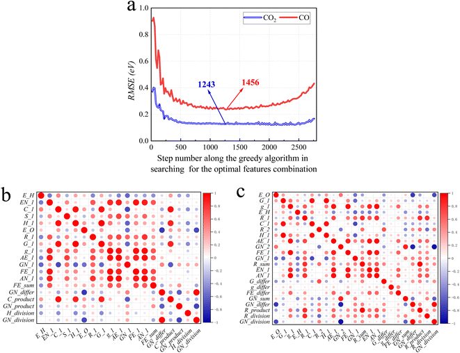
Following the greedy algorithm described in Section 2.2, the optimal combination of features is identified. Shown in Fig. 5a is how the overall RMSE changes as the greedy algorithm proceeds from step 1 to step 2775 in search of the optimal combination of features. Details of some typical data points along the curves of Fig. 5a are further provided in ESI Tables S3 and S4.†

Fig. 5 The result of the greedy algorithm of feature selection. (a) RMSE of E_ads of CO₂ and CO as the greedy algorithm proceeds. (b) and (c), correlation heatmap of optimal combinations of features for CO₂ and CO, respectively. Red and blue indicate positive and negative correlations, respectively. And the sizes of the circles represent the extent of correlation.

For example, as shown in Table S5,† at the earliest stage, the greedy algorithm has located feature 2 (E_H: E_ads of H on alloys) to be the one most correlated to E_ads of CO. At step 136, the algorithm finds that feature 2 together with 63 (EN_1: electronegativity of M1) is the best two-feature combination that can be correlated to E_ads of CO. The mechanism of the following steps is similar.

The lowest RMSE values for E_ads of CO₂ are observed at step number 1243, with a value of 0.11 eV. At this step, 24 features (E_O, FE_1, GN_1, E_H, FE_differ, EN_1, GN_product, G_differ, R_1, GN_2, C_1, R_2, GN_sum, g_differ, R_product, GN_division, R_sum, AN_1, R_division, GN_differ, H_1, AE_1, G_1 and g_1) are in the optimal combination. After this step, when more features are added to this combination, there is a decline in model performance, as indicated by an increase in RMSE. These results suggest that an increasing number of features leads to overfitting with the error reaching 0.18 eV at step 2775. In other words, if all 74 features were considered as the input of the ML model, the performance would be worse than just using the 24 features subset.

For CO the optimal features searching process is similar. At step 1456 the algorithm locates an optimal combination of 19 features (E_H, EN_1, C_1, GN_division, FE_1, E_O, AN_1, AE_1, GN_1, H_division, H_1, GN_product, R_1, C_product, FE_sum, G_1, g_1, GN_differ and S_1), with a minimal RMSE of 0.24 eV.

Fig. 5b and c show the correlation of feature screening results through thermal maps. If the correlation between features is too high, there will be redundant data and waste of learning costs, so the relationship between data can be more intuitively understood. The analysis of the selected features shows that the correlation between them is not dense and high, so the data need not be cleaned.

3.3. Results of the learning algorithms

ML-based and other learning algorithms can provide a cost-effective and efficient CO₂/CO adsorption energy prediction. The primary motivation behind CO₂/CO adsorption energy prediction modeling is using learning algorithms to accelerate the efficiency and reduce computing costs of quantization operations and ensure that results are readily available for the experiment. Tables 2–4 describe the hyperparameters optimization based on different machine learning algorithms.⁵⁹ For MLP: N_l (1–5), L_r (0.00001–1), N_n (1–1000), D_t (0-1) and L₂ (0.00001–1). For DTR: D_m (1–15), S_l (1–10), and S_s (0–1). For SVR: kernel, C (1–32), and epsilon (0.0001–0.5) were optimized using a mixture of exhaustive and dichotomous optimization algorithms in addition to cross-validation and using multi-process concurrency, GPU acceleration, and multi-server operation acceleration methods.

Table 2 MLP model hyperparameter optimization

Adsorption model	Nl	Nn	Lr	Dt	L2	R^2
CO	1	70	0.02	0.01	0.001	0.950
	2	70/25	0.007	0.01	0.0008	0.953
	3	70/25/15	0.006	0.01	0.0007	0.961
	4	70/25/15/375	0.005	0.01	0.0006	0.932
	5	70/25/15/375/215	0.03	0.01	0.0002	0.914
CO2	1	150	0.05	0.01	0.002	0.883
	2	150/175	0.05	0.01	0.001	0.886
	3	150/175/125	0.006	0.01	0.0008	0.908
	4	150/175/125/230	0.0008	0.01	0.00001	0.910
	5	150/175/125/230/400	0.006	0.01	0.00063	0.891

---

Table 3 DTR model hyperparameter optimization

Adsorption model	Dm	Sl	Ss	R^2
CO	1	6	1	0.522
	4	1	0.3	0.854
	8	1	0.3	0.864
	11	1	0.1	0.867
	14	1	0.2	0.861
CO2	1	4	0.6	0.621
	4	1	0.2	0.814
	8	1	0.2	0.796
	11	1	0.3	0.790
	14	1	0.3	0.785

---

Table 4 SVR model hyperparameter optimization

Adsorption model	Kernel	C	Epsilon	R^2
CO	Linear	32	0.5	0.651
	Poly	8	0.1	0.968
	Rbf	16	0.001	0.951
	Sigmoid	2	0.1	0.215
CO2	Linear	3	0.2	0.762
	Poly	5	0.01	0.944
	Rbf	1	0.0001	0.945
	Sigmoid	5	0.02	0.275

---

It should be added that XGBoost does not require hyper-parameter optimization due to its reinforcement learning mechanism. All the learning algorithms performed well in both the training and validation phases, which indicates the model's ability to capture and explain the reasonable variability portion of the dataset.

The intelligent learning algorithms equally depict higher R² values, ranging from 0.867 to 0.968 in the CO modeling and 0.814 to 0.945 in the CO₂ modeling, respectively, representing a higher relation between the experimental and simulated values for the optimized parameter model. Fig. 6 shows that the techniques indicate MAE for a single material value ranging from 0.01 eV to 0.50 eV in the CO₂ modeling and 0.01 eV to 0.75 eV in the CO modeling, respectively, demonstrating a slight deviation between the experimental and simulated values, except DTR model. Generally, according to the objective indices (R², MAE, and RMSE) used in the current study, we can deduce that all the models have performed well in modeling, with some performing better than others. However, the SVR model, composed of all the input variables, performed better than others in most instances in both the training and validation stages. It is worth mentioning that even the XGBoost and MLP techniques equally depict exceptional prediction skills in both the training and validation steps. Furthermore, the performance of the best intelligent combination can be illustrated graphically using different visualizations. The diagram makes it easier to judge how well other datasets or models represent the variation and patterns in the reference dataset. Moreover, the prediction skills of the learning algorithms can also be visualized using the scatter plot, a popular data visualization style, as demonstrated in Fig. 6. A complete picture of how well several models or datasets compare to a reference dataset in terms of correlation is provided by scatter plot. A better agreement with the reference dataset is indicated by points nearer the reference point regarding these criteria. A two-dimensional graph consists of points plotted with one variable on the x-axis and the other on the y-axis. The positions of the two variables being compared indicate where each point in the dataset, representing an observation or data point, is located. Hence, the scatter plot performance depicts the graphical illustration of the table's optimal result. Therefore, the performance of the models should be ordered by SVR > MLP > XGBoost > DTR.

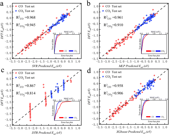Fig. 6 The predicted CO₂/CO adsorption energies by ML algorithms versus DFT results for (a) SVR, (b) MLP, (c) DTR, and (d) XGBoost.

3.4. Validation of the learning algorithms

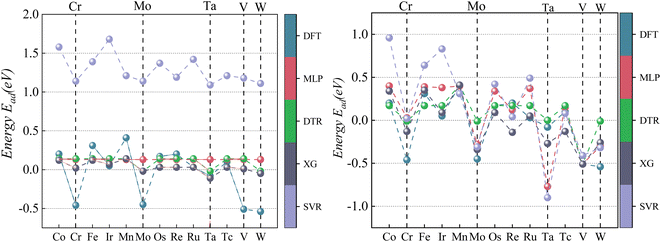
The machine learning model proposed in this study can accurately predict the adsorption energy of alloys with given physical and chemical characteristics, and the verification is divided into two parts. Firstly, the validity of this prediction model has been tested against all alloys included in the training set as shown in Fig. 6. Secondly, the model was applied to predict the adsorption energy on unknown alloys as verification. During the verification stage, we selected only Pd and Rh to test the predictive ability of the model. Although only Pd and Rh were considered in this study, our model is applicable to all binary alloy materials. Once we verified the stability of the model, the next step can be a large-scale material screening. The main reason to select Pd at this stage is that Pd alloys have been shown to be able to achieve high selectivity for CO₂ reduction to CO. For example, Li et al. prepared CuPd alloys and used DFT calculations to show that Pd atoms in CuPd alloys act as reaction centers and possess strong adsorption affinity with COOH.⁶⁰ Adjacent Cu atoms enhance their catalytic performance by changing the electronic structure and atomic arrangement of Pd. Ma et aldiscovered that the selectivity of CO₂RR products is affected by the atom mixing state of CuPd bimetallic catalysts.⁶¹ The selection of doping atoms is consistent with the previous sections (Co, Cr, Fe, Ir, Mn, Mo, Os, Re, Ru, Ta, Tc, V, and W).

Since Pd base data did not participate in the learning training, we adopted two prediction modes: prediction 1: Including only the 78 alloy data into the XGBoost model for prediction. Prediction 2: supplement with adsorption data on two additional Pd-doped alloys to the training set of data 1, and reform the learning process before making predictions. In prediction 2, extra information about the Pd base materials was provided to train the ML model to improve the prediction accuracy. The reason to use this method in this study is that if unknown base data learning is not provided, direct prediction (prediction 1) may have an explosion of dimensions. For example, one of the features is the atomic number of the dopant atom. When the previously learned model is applied to a new alloy, the atomic number of the new model may be out of range of the previously learned data set. If the values of a significant number of features are outside the range, there will be a considerable error. Results of these two predictions on the Pd alloys are listed in Tables 5 and 6 and visualized in Fig. 7 and 8. Similar results for Rh alloys are provided in ESI Tables S5, S6, Fig. S4 and S5.†

Table 5 Results of four machine learning algorithms for predicting CO₂ adsorption energy based on Pd alloys

Algorithms and results		Co	Cr	Fe	Ir	Mn	Mo	Os	Re	Ru	Ta	Tc	V	W	MAE (eV)
a These cases are part of the training set; therefore, small errors are expected.b Error between DFT and predicted value.
DFT (eV)		0.20	−0.46	0.31	0.05	0.41	−0.45	0.17	0.20	0.03	−0.08	0.10	−0.51	−0.54
MLP	Prediction 1 (eV)	0.13	0.13	0.13	0.13	0.13	0.13	0.13	0.13	0.13	0.13	0.13	0.13	0.13	0.27
	Error (eV)^b	0.07	−0.59	0.18	−0.08	0.28	−0.58	0.04	0.07	−0.10	−0.21	−0.03	−0.64	−0.67
	Prediction 2 (eV)	0.40	0.03	0.39	0.38	0.40	−0.28	0.34	0.12	0.37	−0.17	0.15	−0.51	−0.30	0.22
	Error (eV)^b	−0.20	−0.49	−0.08	−0.33	−0.01^a	−0.17	−0.17	0.08	−0.34	0.09	−0.05	0.00^a	−0.24
DTR	Prediction 1 (eV)	0.14	0.14	0.14	0.14	0.14	−0.02	0.14	0.14	0.14	−0.02	0.14	0.14	−0.02	0.24
	Error (eV)^b	0.06	−0.60	0.17	−0.09	0.27	−0.43	0.03	0.06	−0.11	−0.06	−0.04	−0.65	−0.52
	Prediction 2 (eV)	0.17	−0.01	0.17	0.17	0.41	−0.01	0.17	0.17	0.17	0.00	0.17	−0.51	−0.01	0.16
	Error (eV)^b	0.03	−0.45	0.14	−0.12	0.00^a	−0.44	0.00	0.03	−0.14	−0.08	−0.07	0.00^a	−0.53
XG	Prediction 1 (eV)	0.12	0.02	0.12	0.07	0.14	−0.02	0.03	0.03	0.03	−0.11	0.03	0.01	−0.05	0.22
	Error (eV)^b	0.08	−0.48	0.19	−0.02	0.27	−0.43	0.14	0.17	0.00	0.03	0.07	−0.52	−0.49
	Prediction 2 (eV)	0.34	−0.13	0.35	0.09	0.41	−0.34	0.09	−0.14	0.05	−0.27	−0.13	−0.51	−0.26	0.14
	Error (eV)^b	−0.14	−0.33	−0.04	−0.04	0.00^a	−0.11	0.08	0.34	−0.02	0.19	0.23	0.00^a	−0.28
SVR	Prediction 1 (eV)	1.58	1.14	1.39	1.68	1.21	1.14	1.37	1.19	1.42	1.09	1.21	1.18	1.11	1.33
	Error (eV)^b	−1.38	−1.60	−1.08	−1.63	−0.80	−1.59	−1.20	−0.99	−1.39	−1.17	−1.11	−1.69	−1.65
	Prediction 2 (eV)	0.96	0.02	0.64	0.83	0.31	−0.31	0.42	0.04	0.49	−0.90	0.08	−0.41	−0.32	0.36
	Error (eV)^b	−0.76	−0.48	−0.33	−0.78	0.10^a	−0.14	−0.25	0.16	−0.46	0.82	0.02	−0.10^a	−0.22

---

Table 6 Results of four machine learning algorithms for predicting CO adsorption energy based on Pd alloys

Algorithms and results		Co	Cr	Fe	Ir	Mn	Mo	Os	Re	Ru	Ta	Tc	V	W	MAE (eV)
a These cases are part of the training set; therefore, small errors are expected.b Error between DFT and predicted value.
DFT (eV)		−2.13	−1.63	−2.14	−2.47	−1.94	−1.43	−2.37	−1.87	−2.28	−1.04	−1.88	−1.26	−1.45
MLP	Prediction 1 (eV)	−1.97	−1.69	−2.03	−1.99	−1.88	−1.55	−2.12	−1.93	−1.98	−1.08	−1.85	−1.16	−1.61	0.15
	Error (eV)^b	−0.16	0.05	−0.11	−0.48	−0.06	0.12	−0.25	0.06	−0.30	0.04	−0.03	0.10	0.16
	Prediction 2 (eV)	−2.05	−1.72	−2.06	−2.06	−1.92	−1.63	−2.21	−1.97	−2.02	−1.20	1.92	−1.24	−1.74	0.14
	Error (eV)^b	−0.08	0.09	−0.08	−0.41	−0.02^a	0.20	−0.16	0.10	−0.26	0.16	−0.04	−0.02^a	0.29
DTR	Prediction 1 (eV)	−2.19	−2.19	−2.19	−2.36	−1.88	−1.63	−2.69	−2.69	−2.36	−0.66	−1.88	−1.29	−1.63	0.22
	Error (eV)^b	0.06	0.56	0.05	−0.11	−0.06	0.20	0.32	0.82	0.08	−0.38	0.00	0.03	0.18
	Prediction 2 (eV)	−2.13	−2.13	−2.13	−2.41	−1.88	−1.63	−2.41	−2.41	−2.41	−0.66	−1.90	−1.29	−1.63	0.18
	Error (eV)^b	0.00	0.50	−0.01	−0.06	−0.06^a	0.20	0.04	0.54	0.13	−0.38	0.02	0.03^a	0.18
XG	Prediction 1 (eV)	−2.11	−1.65	−2.10	−2.25	−1.90	−1.63	−2.18	−1.88	−2.21	−1.00	−1.85	−1.28	−1.53	0.08
	Error (eV)^b	−0.02	0.02	−0.04	−0.22	−0.04	0.20	−0.19	0.01	−0.07	−0.04	−0.03	0.02	0.08
	Prediction 2 (eV)	−2.14	−1.67	−2.12	−2.26	−1.94	−1.64	−2.19	−2.00	−2.23	−1.04	−1.85	−1.26	−1.53	0.07
	Error (eV)^b	0.01	0.04	−0.02	−0.21	0.00^a	0.21	−0.18	0.13	−0.05	0.00	−0.03	0.00^a	0.08
SVR	Prediction 1 (eV)	−2.29	−2.19	−2.39	−2.48	−2.33	−2.07	−2.75	−2.50	−2.38	−1.83	−2.34	−1.74	−2.29	0.44
	Error (eV)^b	0.16	0.56	0.25	0.01	0.39	0.64	0.38	0.63	0.10	0.79	0.46	0.48	0.84
	Prediction 2 (eV)	−2.06	−1.90	−2.13	−2.22	−1.94	−1.74	−2.44	−2.2	−2.13	−1.4	−2.09	−1.26	−1.94	0.19
	Error (eV)^b	−0.07	0.27	−0.01	−0.25	0.00^a	0.31	0.07	0.33	−0.15	0.36	0.21	0.00^a	0.49

---

Fig. 7 Comparison of CO E_ads between four ML predictions and DFT ML models and DFT: prediction 1 (left); prediction 2 (right). Vertical lines mark the alloys with the five lowest E_ads calculated by DFT.

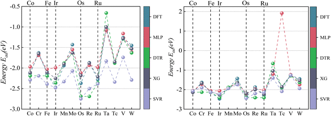Fig. 8 Comparison of CO₂ E_ads between four ML predictions and DFT: prediction 1 (left); prediction 2 (right).

According to the data analysis of CO₂ adsorption energy in Table 5, prediction 1 shows that the MLP model has the most significant deviation with a maximum error of −0.67 eV for a single material, a minimum error of −0.03 eV for a single material, and an MAE of 0.272 eV for all materials. The XGBoost model has the least deviation with a maximum error of −0.52 eV for a single material, a minimum error of 0 eV for a single material, and an MAE of 0.223 eV for all materials. This result is mainly due to machine learning being derived from learned data. If feature laws do not conform to the learned set outside this range, it may lead to prediction bias. Unlearned Pd data can affect prediction accuracy if there is a significant deviation between primary Pd data and learning sets.

After learning and training from CO₂ adsorption energy characteristic data on Pd/Mn and Pd/V alloys, prediction 2 results show significantly improved accuracy across all four machine learning models compared to prediction 1 results alone. Among them, XGBoost has the best prediction accuracy on CO₂ adsorption energy, with its the MAE decreased from 0.223 eV to 0.138 eV.

As visualized in Fig. 7, With the five Eads lowest energy calculated by DFT are Pd/W, Pd/V, Pd/Cr, Pd/Mo, and Pd/Ta. The predicted results of XGBoost are Pd/Ta, Pd/W, Pd/Mo, Pd/V and Pd/Cr. Although the expected adsorption energy values were somewhat skewed, the lowest five energy combinations were 100% accurate.

According to the CO adsorption energy data analysis in Table 6 and Fig. 8, MLP and XGBoost have excellent performance regardless of prediction 1 or 2, while DTR and SVR have average performance. The main reason for the difference in predicted results between CO and CO₂ is that the adsorption energy of the vital feature H is positively correlated with the adsorption energy value of CO, therefore even the prediction of the unknown base data also conforms to this law with a small error. The XGBoost model has the best prediction effect on CO adsorption energy. As shown in Fig. 8, the five alloy combinations with the lowest energy calculated by DFT are Pd/Ir, Pd/Os, Pd/Ru, Pd/Fe, and Pd/Co. The prediction 1 results of XGBoost are Pd/Ir, Pd/Ru, Pd/Os, Pd/Co, and Pd/Fe.

To sum up, the result of prediction 1 is XGBoost > MLP = SVR = DTR, and the result of prediction 2 is XGBoost = MLP > SVR = DTR. Although the MLP and SVR models have strong learning abilities, their generalization of data processing is poor. Therefore, the XGBoost model is still the most stable machine learning model for the prediction of adsorption energy.

3.5. Screening potential catalysts for CO₂ generation to CO

Developing cheap, active, and stable catalysts is the goal of catalyst researchers. CO₂, COOH, and CO adsorption energy are suggested as the best descriptors for CO₂ hydrogenation to CO; Based on the results of Wang's study,⁶² the limiting potential of binary alloys CO₂ reduction to CO by considering reaction pathways R1, R2, and R3 as following:

COOH* + (H⁺ + e⁻) → CO* + H₂O (R3)

where * represents an empty site on the metal or alloy surface.

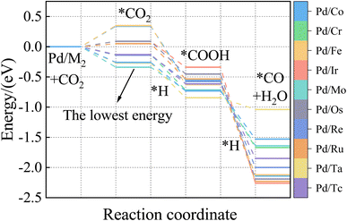
The ML model can predict the adsorption energy values of CO₂, and CO on all alloy surfaces, and based on the stability of reaction intermediates, a potential energy diagram along the CO₂ reduction reaction pathway can be constructed and shown in Fig. 9. It should be noted that our model predicts only the E_ads of CO and CO₂, there E_ads of the intermediate COOH on Fig. 9 were directly from DFT calculations. In the future, our model can be extended to predict E_ads of all intermediates along the CO₂RR pathway. Meanwhile, our model lacks the ability to estimate kinetic barriers, and the energies shown in Fig. 9 are only electronic energies without entropy or zero-point corrections. Despite these limitations, this model provides useful information in the screening of materials. Specifically, our model predicts that Pd/Mo may provide a fast CO₂ to COOH conversion because of its strong binding to both CO₂ and COOH. Although Pd/Os also has a strong binding with COOH, its weak binding of CO may lead to the conversion to CO slower than Pd/Os.

Fig. 9 Potential energy diagram along CO₂ reduction pathway predicted by XGBoost.

To our knowledge, there are no reports about Pd/Mo alloy catalysts for CO₂RR. But the Pd/Mo alloy, a highly curved and sub-nanometer thick metal nanosheet, is an efficient and stable electrocatalyst for ORR and OER in alkaline electrolytes and has shown good performance in zinc-air and lithium-air batteries,⁶³ Dawid Ciesielski et al. studied the diffusion of Pd adatoms on faceted Pd/Mo (111) surfaces with hill and valley structures is studied using the kinetic Monte Carlo method.⁶⁴ Cao⁶⁵ et al. also describe an efficient method for preparing highly dispersed carbon-supported Pd/Mo bimetallic nanoparticles. In other words, as a preliminary screening result, the selected alloy catalysts need to be further verified. Nevertheless, if the CO and CO₂ adsorption energies and stability of layered alloys play a vital role in a process like CO₂ hydrogenation to CO provided in this paper, it will be very informative and valuable.

4 Conclusion

In this paper, CO_2, CO, H, and O adsorption energies on 78 single-atom doped alloys were calculated using PBE functional and slab models. Based on these DFT calculated adsorption energies, XGBoost machine learning models were established using non-quantum and quantum chemistry features. To overcome overfitting and reduce feature dimension, we performed a modified feature selection process by using the greedy algorithm. With this algorithm, we examined the performance of ML models at different feature subsets. The features selected were used in the modified XGBoost algorithm. The MAE is 0.075 eV for the CO model of the adsorption energies and 0.138 eV for the CO₂ model of the adsorption energies.

In the future, the ML model will be further improved by expanding the optimization of descriptors, adding ensemble learning methods, and expanding the data set. At the same time, this method can also be applied to the screening of electrocatalytic materials by predicting the adsorption energy of all intermediate products in the alloy catalytic electroreduction pathway of carbon dioxide reduction.

Author contributions

Conceptualization, X. Cao and W. Luo; methodology, X. Cao, and W. Luo; formal analysis, X. Cao, and H. Liu; writing—original, X. Cao; writing—review, and editing, X. Cao, and W. Luo. All authors have read and agreed to the published version of the manuscript.

Conflicts of interest

The authors declare no conflict of interest.

References

1. S. Zaman and S. Chen, J. Catal., 2023, 421, 221–227.
2. A. Pytlak, A. Szafranek-Nakonieczna, W. Goraj, I. Śnieżyńska, A. Krążała, A. Banach, I. Ristović, M. Słowakiewicz and Z. Stępniewska, Sci. Total Environ., 2021, 800, 149551.
3. P. Tcvetkov, Energies, 2021, 14, 411.
4. S. S. Bhattacharyya, F. F. G. D. Leite, M. A. Adeyemi, A. J. Sarker, G. S. Cambareri, C. Faverin, M. P. Tieri, C. Castillo-Zacarías, E. M. Melchor-Martínez and H. M. Iqbal, Sci. Total Environ., 2021, 790, 148169.
5. H. L. Vu, K. T. W. Ng and D. Bolingbroke, Waste Manage., 2019, 84, 129–140.
6. D. D. Zhu, J. L. Liu and S. Z. Qiao, Adv. Mater., 2016, 28, 3423–3452.
7. C. Kim, F. Dionigi, V. Beermann, X. Wang, T. Möller and P. Strasser, Adv. Mater., 2019, 31, 1805617.
8. T.-r. Wang, J.-c. Li, W. Shu, S.-l. Hu, R.-h. Ouyang and W.-x. Li, Chin. J. Chem. Phys., 2020, 33, 703–711.
9. W. Yu, M. D. Porosoff and J. G. Chen, Chem. Rev., 2012, 112, 5780–5817.
10. M. Escudero-Escribano, P. Malacrida, M. H. Hansen, U. G. Vej-Hansen, A. Velázquez-Palenzuela, V. Tripkovic, J. Schiøtz, J. Rossmeisl, I. E. Stephens and I. Chorkendorff, Science, 2016, 352, 73–76.
11. L. Tong, Z. Jin-Qin, A. Mao-Zhong, Y. Pei-Xia and W. Peng, Chin. J. Inorg. Chem., 2017, 33, 1587–1594.
12. S. Yu, H. Chai, Y. Xiong, M. Kang, C. Geng, Y. Liu, Y. Chen, Y. Zhang, Q. Zhang and C. Li, Adv. Mater., 2022, 34, 2200908.
13. X. Zhi, A. Vasileff, Y. Zheng, Y. Jiao and S.-Z. Qiao, Energy Environ. Sci., 2021, 14, 3912–3930.
14. J. Chen and L. Wang, Adv. Mater., 2022, 34, 2103900.
15. Y. Hu, H. Li, Z. Li, B. Li, S. Wang, Y. Yao and C. Yu, Green Chem., 2021, 23, 8754–8794.
16. Z. Mi, X. Fan, T. Li, L. Yang, H. Su, W. Cai, S. Li and G. Zhang, Processes, 2023, 11, 3241.
17. J.-C. Jiang, J.-C. Chen, M.-d. Zhao, Q. Yu, Y.-G. Wang and J. Li, Nano Res., 2022, 15, 7116–7123.
18. F. Calle-Vallejo, J. Martínez, J. M. García-Lastra, J. Rossmeisl and M. Koper, Phys. Rev. Lett., 2012, 108, 116103.
19. X. Zhong, B. Gallagher, S. Liu, B. Kailkhura, A. Hiszpanski and T. Y.-J. Han, npj Comput. Mater., 2022, 8, 204.
20. Z. Sun, H. Yin, K. Liu, S. Cheng, G. K. Li, S. Kawi, H. Zhao, G. Jia and Z. Yin, SmartMat, 2022, 3, 68–83.
21. P. Wang, T. Weise and R. Chiong, Evol. Intell., 2011, 4, 3–16.
22. T. Hastie, R. Tibshirani, J. H. Friedman and J. H. Friedman, The Elements of Statistical Learning: Data Mining, Inference, and Prediction, Springer, 2009.
23. B. B. Goldman and W. P. Walters, Annu. Rep. Comput. Chem., 2006, 2, 127–140.
24. Q. Zhang, R. Zeng, Y. Lu, J. Zhang, W. Zhou and J. Yu, New J. Chem., 2022, 46, 10451–10457.
25. J. G. T. Tomacruz, K. E. S. Pilario, M. F. M. Remolona, A. A. B. Padama and J. D. Ocon, Chem. Eng. Trans., 2022, 94, 733–738.
26. R. A. Hoyt, M. M. Montemore, I. Fampiou, W. Chen, G. Tritsaris and E. Kaxiras, J. Chem. Inf. Model., 2019, 59, 1357–1365.
27. S. Agarwal and K. Joshi, ChemistrySelect, 2022, 7, e202202414.
28. T.-T. Shi, G.-Y. Liu and Z.-X. Chen, J. Phys. Chem. C, 2023, 127, 9573–9583.
29. F. Liu, P. F. Gao, C. Wu, S. Yang and X. Ding, ChemPhysChem, 2023, 24, e202200642.
30. S. Nayak, S. Bhattacharjee, J.-H. Choi and S. C. Lee, J. Phys. Chem. A, 2019, 124, 247–254.
31. X. Li, B. Li, Z. Yang, Z. Chen, W. Gao and Q. Jiang, J. Mater. Chem. A, 2022, 10, 872–880.
32. W. Malone and A. Kara, Surf. Sci., 2023, 731, 122252.
33. V. Fung, G. Hu, P. Ganesh and B. G. Sumpter, Nat. Commun., 2021, 12, 88.
34. X. Li, X. Zhang, J. Zhang, J. Gu, S. Zhang, G. Li, J. Shao, Y. He, H. Yang and S. Zhang, Carbon Capture Sci. Technol., 2023, 9, 100146.
35. K. Tran and Z. W. Ulissi, Nat. Catal., 2018, 1, 696–703.
36. R. Gasper, H. Shi and A. Ramasubramaniam, J. Phys. Chem. C, 2017, 121, 5612–5619.
37. J. Edmonds, Math. Program., 1971, 1, 127–136.
38. T. A. Batchelor, J. K. Pedersen, S. H. Winther, I. E. Castelli, K. W. Jacobsen and J. Rossmeisl, Joule, 2019, 3, 834–845.
39. G. Kresse and J. Furthmüller, Comput. Mater. Sci., 1996, 6, 15–50.
40. M. C. Payne, M. P. Teter, D. C. Allan, T. Arias and a. J. Joannopoulos, Rev. Mod. Phys., 1992, 64, 1045.
41. H. J. Monkhorst and J. D. Pack, Phys. Rev. B: Solid State, 1976, 13(12), 5188–5192.
42. P. Fabian, J. Mach. Learn. Res., 2011, 12, 2825.
43. T. Bartz-Beielstein, arXiv, 2023, preprint, arXiv:2305.11930,  DOI:10.48550/arXiv.2305.11930.
44. L. Yang and A. Shami, Neurocomputing, 2020, 415, 295–316.
45. S. Hayou, A. Doucet and J. Rousseau, arXiv, 2019, preprint, arXiv:1905.13654,  DOI:10.48550/arXiv.1905.13654.
46. Y. Yu, K. Adu, N. Tashi, P. Anokye, X. Wang and M. A. Ayidzoe, IEEE Access, 2020, 8, 72727–72741.
47. J. Schmidt, Hieber, 2020, 48(4), 1875–1897.
48. S. Yuan, Y. Zhang, J. Tang, W. Hall and J. B. Cabotà, Artif. Intell. Rev., 2020, 53, 843–874.
49. W. Zhou, L. Zhang and L. Jiao, Pattern Recognit., 2002, 35, 2927–2936.
50. A. Pathy, S. Meher and P. Balasubramanian, Algal Res., 2020, 50, 102006.
51. M.-E. Ragoussi and S. Brassinnes, Radiochim. Acta, 2015, 103, 679–685.
52. J. G. T. Tomacruz, K. E. S. Pilario, M. F. M. Remolona, A. A. B. Padama and J. D. Ocon, Chem. Eng. Trans., 2022, 94, 733–738.
53. W. Ma, S. Xie, X.-G. Zhang, F. Sun, J. Kang, Z. Jiang, Q. Zhang, D.-Y. Wu and Y. Wang, Nat. Commun., 2019, 10, 892.
54. M. S. Lei Xia, H. Li, W. Zhang, Y. Cheng and X.-Q. Xia, Biology, 2024, 13, 100.
55. R. Zhang and Y. Ding, Curr. Comput.-Aided Drug Des., 2020, 16, 725–733.
56. D. Wu, J. Zhang, M.-J. Cheng, Q. Lu and H. Zhang, J. Phys. Chem. C, 2021, 125, 15363–15372.
57. M. Sarveghadi, A. H. Gandomi, H. Bolandi and A. H. Alavi, Neural Comput. Appl., 2019, 31, 2085–2094.
58. A. A. Shahmansouri, H. A. Bengar and E. Jahani, Constr. Build. Mater., 2019, 229, 116883.
59. Y. A. Ali, E. M. Awwad, M. Al-Razgan and A. Maarouf, Processes, 2023, 11, 349.
60. M. Li, J. Wang, P. Li, K. Chang, C. Li, T. Wang, B. Jiang, H. Zhang, H. Liu, Y. Yamauchi, N. Umezawa and J. Ye, J. Mater. Chem. A, 2016, 4, 4776–4782.
61. S. Ma, M. Sadakiyo, M. Heima, R. Luo, R. T. Haasch, J. I. Gold, M. Yamauchi and P. J. A. Kenis, J. Am. Chem. Soc., 2017, 139, 47–50.
62. D. Wang, R. Cao, S. Hao, C. Liang, G. Chen, P. Chen, Y. Li and X. Zou, Green Energy Environ., 2023, 8, 820–830.
63. M. Luo, Z. Zhao, Y. Zhang, Y. Sun, Y. Xing, F. Lv, Y. Yang, X. Zhang, S. Hwang and Y. Qin, Nature, 2019, 574, 81–85.
64. D. Ciesielski and C. Oleksy, Surf. Sci., 2012, 606, 1481–1488.
65. C. Cao, G. Yang, W. Song, X. Ju, Q. Hu and J. Yao, J. Power Sources, 2014, 272, 1030–1036.

---

Footnote

† Electronic supplementary information (ESI) available: Supplementary materials (including adsorption energy calculated by VASP, concrete values of machine learning feature parameters, the full name and naming of physicochemical parameters, and the feature screening results) are available in this article. Source codes of our ML models can be available to readers upon request. See DOI: https://doi.org/10.1039/d4ra00710g

---