Advanced analytical methods for multi-spectral transmission imaging optimization: enhancing breast tissue heterogeneity detection and tumor screening with hybrid image processing and deep learning

Abstract

Light sources exhibit significant absorption and scattering effects during the transmission through biological tissues, posing challenges in identifying heterogeneities in multi-spectral images. This paper introduces a fusion of techniques encompassing the spatial pyramid matching model (SPM), modulation and demodulation (M_D), and frame accumulation (FA). These techniques not only elevate image quality but also augment the precision of heterogeneous classification in multi-spectral transmission images (MTI) within deep learning network models (DLNM). Initially, experiments are designed to capture MTI of phantoms. Subsequently, the images are preprocessed separately through a combination of different techniques such as SPM, M_D and FA. Ultimately, multi-spectral fusion pseudo-color images derived from U-Net semantic segmentation are fed into VGG16/19 and ResNet50/101 networks for heterogeneous classification. Among them, different combinations of SPM, M_D and FA significantly enhance the quality of images, facilitating the extraction of heterogeneous feature information from multi-spectral images. In comparison to the classification accuracy achieved in the original image VGG and ResNet network models, all images after preprocessing effectively improved the classification accuracy of heterogeneities. Following scatter correction, images processed with 3.5 Hz modulation-demodulation combined with frame accumulation (M_D-FA) attain the highest classification accuracy for heterogeneities in the VGG19 and ResNet101 models, achieving accuracies of 95.47% and 98.47%, respectively. In conclusion, this paper utilizes different combinations of SPM, M_D and FA techniques to not only enhance the quality of images but also further improve the accuracy of DLNM in heterogeneous classification, which will promote the clinical application of MTI technique in breast tumor screening.

---

1. Introduction

Breast cancer has now surpassed lung cancer as the most prevalent malignancy worldwide, with an annual incidence rate of up to 11.7%.¹ Among women in China, it stands as the most common malignant tumor, and its incidence continues to climb. Regular screening is an effective method to detect tumors and improve the prognosis of patients. Prompt treatment of breast cancer not only protects the female breast tissue to the greatest extent, but also significantly improves the cure rate.² However, the physical structure of breast tumors is often indistinct in medical images, making it difficult to identify and locate tumors within breast tissue in terms of position and size. For example, X-rays commonly used in clinical practice are not routinely used to screen for breast cancer, mainly because when X-rays irradiate human tissues, they will react with substances in the tissues, destroy the cellular structure of human tissues, and cause permanent damage to human tissues. Additionally, X-ray examinations have relatively low sensitivity for dense breast tissue in younger women.³ Ultrasound imaging lacks standardized protocols and is time-consuming, with diagnostic accuracy hinging on the skill and experience of the technician.⁴ Computed Tomography (CT) takes a long time to scan, and only a limited number of layers can be scanned during the effective time of contrast agent, which cannot guarantee spatial resolution of images.⁵ Magnetic Resonance Imaging (MRI) is slow, costly and insensitive to calcifications and cortical bone lesions, posing challenges for quantitative diagnosis.⁶

In recent years, optical imaging has gradually become a research hotspot and has been widely applied in many fields. In comparison to conventional clinical imaging methods, optical imaging methods possess the following significant advantages:⁷ (a) it utilizes safe, non-ionizing radiation and non-invasive methods to detect tissues. (b) It displays contrast between soft tissues based on the optical properties of tissues. (c) It can be used for continuous monitoring of tissue lesions. (d) It offers high spatial resolution (lateral resolution less than 1 micron in the visible range). Moreover, breast tissue is semi-transparent and highly transmissibility. During optical transmission imaging, the abundance of neovascularization and hemoglobin surrounding breast tumor tissues results in significant shadows, termed heterogeneities.⁸ Therefore, optical transmission imaging provides a clinically non-invasive detection method for screening breast cancer.

Multi-spectral non-destructive transmission optical imaging has become a research hotspot due to its real-time, non-invasive, safe, specific and highly sensitive advantages, and has been widely applied in many fields.^9,10 However, there is relatively limited research on the application of multi-spectral transmission images (MTI) in medical field. This is mainly due to the absorption and scattering characteristics of tissues, which strictly limit the transmission depth of light sources. During transmission, light is absorbed by water, macromolecules (like proteins), and pigments (such as melanin and hemoglobin) in biological tissues, leading to photon loss and image dimming. The presence of these components restricts the propagation of light, making it difficult to obtain high-information images. Currently, modulation-demodulation (M_D) and frame accumulation (FA) technologies have become the most effective methods to enhance low-light signals in the process of obtaining MTI with various low-light level image detection devices. Li et al. significantly improved the signal-to-noise ratio (SNR) and resolution of low-light images using FA and shaping signal techniques.^11–13

Additionally, advancements in machine learning and hardware capabilities have led to the widespread application of deep learning-based image object classification methods. Through layer-by-layer convolution, deep learning extracts high-level abstract features from images and uncovers hidden properties within targets, which will facilitate the development of MTI in breast tumor detection, bringing new possibilities to medical diagnosis.^14–16 Recent research efforts have increasingly utilized diverse deep neural networks, including vanilla CNNs,^17,18 ResNet,¹⁹ LSTMs,²⁰ DenseNet,²¹ and transformers,²² to predict malignancy across various imaging modalities. Various studies have indicated that exploring the unique characteristics of different imaging modalities, such as the consistency between medio-lateral oblique (MLO) and cranio-caudal (CC) views in digital mammography (DM) and the layer variations in breast anatomical structures in ultrasound images, can significantly enhance classification accuracy.²³ However, a significant challenge faced by DL methods is their heavy reliance on extensive training data, which is often scarce in the medical domain and can lead to overfitting. To mitigate this issue, transfer learning has been widely adopted.^24,25 This approach leverages pre-trained parameters from renowned networks like VGG16, ResNet50, and AlexNet, which were initially trained on natural images, serving as encoder initializations for fine-tuning. Experimental findings have demonstrated that incorporating prior knowledge from other domains can substantially improve the performance of breast cancer classification tasks.^26,27 Among them, advancements in breast cancer detection have leveraged digital mammography (DM), digital breast tomosynthesis (DBT), breast ultrasound (US), and magnetic resonance imaging (MRI) techniques. In DM and DBT, recent research has emphasized the development of size-adaptive networks to handle various masses, incorporating strategies such as multi-scale inputs,^28,29 multi-scale features,^30,31 and multi-scale supervisions³² to capture comprehensive information. For breast US images, various neural networks, including RCNNs,³³ U-Nets,^34,35 cascaded U-Nets,³⁶ and GANs,^37,38 have demonstrated promising detection results. Notably, the integration of prior knowledge has enhanced tumor feature exploration, exemplified by Byra et al.'s use of quantitative entropy parametric maps and Li et al.'s dynamic parallel spatiotemporal transformer framework for breast US videos. MRI, with its high sensitivity to detecting lesions with increased intensity in surrounding tissues, has been pivotal in capturing semantic information of lesions.^39,40 Huang et al. proposed joint-phase attention blocks for extracting cancer representations from pre- and post-contrast images,⁴¹ while Wang et al. introduced a tumor-sensitive synthesis module to guide the detection network in learning semantic cancerous features.⁴² Lv et al. further utilized a weight-shared encoder and a spatiotemporal graph to capture dynamics and pharmacokinetics priors for accurate tumor detection.⁴³ In addressing the large-scale nature of whole slide images (WSIs), researchers have adopted patch-wise classification approaches, such as Gecer et al. mapping of patches into cancer categories and Guo et al. application of the Inception-V3 model for classification, followed by refinement in a pixel-wise manner.^44,45 These advancements collectively contribute to improved breast cancer detection and detection accuracy. And as shown in Table 1, a further comprehensive review of the progress of deep learning in breast cancer screening between 2022 and 2024 is provided. During these three years, researchers have explored various neural network architectures and optimization techniques to enhance the performance of these models. Furthermore, efforts have been made to integrate these models into clinical workflows, aiming to improve the efficiency and accuracy of breast cancer screening. However, existing clinical examination techniques struggle to simultaneously meet the characteristics required for breast tumors detection, such as regularity, non-radiation, low cost, convenience and ease of implementation.

Table 1 Summary of deep learning advancements in breast cancer screening classification: 2022–2024

Reference	Methodology	Results	Advantages/shortcomings	Image type
1 (ref. 46)	An interpretable multitask information bottleneck network (MIB-Net)	Accuracy: DES 91.28%, BUSI 92.97%	The method proposed is a double prior knowledge guidance strategy to promote feature representation and improve the performance of regular multitask networks	Mammogram ultrasound breast image
2 (ref. 47)	A novel end-to-end deep learning framework for mammogram image processing	Accuracy: DDSM 85%, INbreast 93%	The proposed approach is constructed in a dual-path architecture, solving the mapping in a two-problem manner, with additional consideration of important shape and boundary knowledge	Mammogram breast image
3 (ref. 48)	WDCCNet: weighted double-classifier constraint neural network for mammographic image classification	Accuracy: private 89.60%	A two-classifier network architecture is developed to constrain the extracted feature distribution by changing the decision boundary of the classifier	Mammogram breast image
4 (ref. 49)	A novel segmentation-to-classification scheme by adding the segmentation-based attention (SBA) information to the deep convolution network (DCNN) for breast tumors classification	Accuracy: private 90.78%	This method integrates the relationship between the two visual tasks of tumor region segmentation and classification	Ultrasound breast image
5 (ref. 50)	A novel deconv-transformer (DecT) network model, which incorporates the color deconvolution in the form of convolution layers	Accuracy: BreakHis 93.02%, BACH 79.06%, UC 81.36%	Color dithering is used to reduce overfitting in the process of image data enhancement	Histology breast image
6 (ref. 51)	A dual-channel ResNet-GAP network is developed, one channel for BUS and the other for EUS.	Accuracy: private 88.60%	The multi-scale consistency of the CAMs in both channels are further considered in network optimization	B-mode ultrasound (BUS) breast image
7 (ref. 52)	A full digital platform by integrating label-free stimulated Raman scattering (SRS) microscopy with weakly-supervised learning for rapid and automated cancer diagnosis on un-labelled breast CNB.	Accuracy: private 95%	Grad-CAM allowed the trained MIL model to visualize the histological heterogeneity	SRS imaging
8 (ref. 53)	A fully automated pipeline system (FAPS) using RefineNet and the Xception + pyramid pooling module (PPM) was developed to perform the segmentation and classification of breast lesions	Accuracy: internal 94.7%, pooled external 94%, prospective 89.1%	The FAPS-assisted strategy improved the performance of radiologists	Contrast enhanced mammography (CEM) breast image
9 (ref. 54)	A novel strategy to generate multi-resolution TCIs in a single ultrasound image, resulting in a multi-data-input learning task	Accuracy: private 92.12%	An improved combined style fusion method suitable for a deep network is proposed, which integrates the advantage of the decision-based and feature-based methods to fuse the information of different views	Ultrasound breast image
10 (ref. 55)	A novel deep multi-magnification similarity learning (DSML) approach	Accuracy: BCSS2021 93.70%	This method can be used to interpret the multi-magnification learning framework and easily visualize the feature representation from low to high dimensions, overcoming the difficulty of understanding cross-magnification information propagation	Histopathological breast image
11 (ref. 56)	This study adopts multimodal microscopic imaging technology combined with deep learning to achieve rapid intelligent diagnosis of breast cancer	Accuracy: pixel level 89.01% decision fusion 87.53%	This method can obtain abundant information of tissue morphology, collagen content and structure in tissue sections	Microscopic imaging
12 (ref. 57)	This method utilizes a new form of artificial intelligence training called federated learning (FL), especially for breast cancer detection	Accuracy: private 95%	A hybridization of this type of training with meta-heuristic and deep learning is aimed to be proposed for breast cancer diagnosis	Mammogram breast image
13 (ref. 58)	A hybrid deep learning bimodal CAD algorithm for the classification of breast lesions using mammogram and ultrasound imaging modalities combined	Accuracy: private 99.35%	The bimodal CAD algorithm can avoid unnecessary biopsies and encourage its clinical application	Mammogram, ultrasound breast image
14 (ref. 59)	A big data-based two-class (i.e., benign or cancer) BC classification model is developed using the deep reinforcement learning (DRL) method	WBCD 98.90%, WDBC 99.02%, WPBC 98.88%	The gorilla troops optimization (GTO) algorithm is employed for the feature selections	Mammogram breast image
15 (ref. 60)	A deep learning based ensemble classifier is proposed for the detection of breast cancer	Accuracy: mini-DDSM 97.75%, BUSI 94.62%, BUSI2 97.50%	The use of residual learning, depthwise separable convolution, and inverted residual bottleneck structure to make the system faster, as well as skip connection to make optimization easier and lastly	Mammogram ultrasound breast image
16 (ref. 61)	A novel framework which consists of a weight accumulation method and a lightweight fast neural network (FastNet) was proposed for tumor fast identification (TFI) in mobile-computer-assisted devices	Accuracy: private 97.34%	Lightweight FastNet is proposed to improve computing efficiency on mobile devices	Histopathology breast image
17 (ref. 62)	The work works by training transformer-based models to learn semantic features in a self-supervised manner to segment digital signals that are inserted into geometric shapes on the original computed tomography (CT) images	Accuracy: private 74.54%	A convolution pyramid vision transformer (CPT) is developed, which utilizes multi-core convolution patch embedding and local space reduction of each layer to generate multi-scale features, capture local information, and reduce computational costs	Computed tomography (CT) breast image
18 (ref. 63)	A new intermediate layer structure which can fully extract feature information is constructed and named DMBANet.	Accuracy: private 98%	The spindle structure is designed as a multi-branch model, and different attention mechanisms are added to different branches	Histopathological breast image
19 (ref. 64)	Key innovations of the approach include preprocessing techniques, advanced filtering, and data augmentation strategies to optimize model performance, mitigating overand under-fitting concerns	Accuracy: private 99%	A significant development is the chaotic Leader Selective filler Swarm optimization (cLSFSO) method, which effectively detects breast-dense lesions by extracting textural and statistical features	Mammogram breast image
20 (ref. 65)	A new computerized architecture based on two novel CNN architectures with Bayesian optimization and feature selection techniques is proposed	Accuracy: private 97.7%	Extracted deep features are optimized using an improved optimization algorithm named simulated annealing controlled position shuffling (SAcPS)	Mammogram breast image
21 (ref. 66)	A collaborative transfer network (CTransNet) for multi-classification of breast cancer histopathological images is proposed	Accuracy: BreaKHis 98.29%	The residual branch extracts target features from pathological images in a collaborative manner	Mammogram breast image
22 (ref. 67)	A reliable deep learning approach for breast cancer diagnosis is proposed using a random search algorithm and DenseNet121-based transfer-learning model	Accuracy: 40× 98.96% 100× 97.62% 200× 97.08% 400× 96.42%	The reliability of proposed approach is achieved by quantifying the uncertainty of model outcomes using conformal prediction method, guarantying user-chosen levels of confidence	Histopathological breast image
23 (ref. 68)	An automatic methodology capable of detecting tumors and classifying their malignancy in a DCE-MRI breast image is proposed	Accuracy: quantitative imaging network 100%	The method can be integrated as a support system for the specialist in treating patients with breast cancer	Magnetic resonance imaging (MRI) breast image
24 (ref. 69)	A novel computer-aided classification approach, mammo-light for breast cancer prediction is proposed	Accuracy: CBISDDSM 99.17% MIAS 98.42%	Preprocessing strategies have been utilized to eradicate the noise and enhance mammogram lesions	Mammogram breast image
25 (ref. 70)	An EfficientNet-integrated ResNet deep network and XAI-based framework for accurately classifying breast cancer (malignant and benign) is proposed	Accuracy: BUSI 98%	A new feature selection technique is proposed based on the cuckoo search algorithm called cuckoo search controlled standard error mean	Ultrasound imaging (BUSI) breast image
26 (ref. 71)	A new deep-learning diagnosis framework, called InterNRL, that is designed to be highly accurate and interpretable is proposed	Accuracy: private 90.37%	The two classifiers are mutually optimised with a novel reciprocal learning paradigm in which the student ProtoPNet learns from optimal pseudo labels produced by the teacher GlobalNet, while GlobalNet learns from ProtoPNet's classification performance and pseudo labels	Mammogram breast image
27 (ref. 72)	This research paper presents the introduction of a feature enhancement method into the Google inception network for breast cancer detection and classification	Accuracy: private 99.81%	A locally preserving projection transformation function is introduced to retain local information that might be lost in the intermediate output of the inception model	Ultrasound breast image
28 (ref. 73)	An efficient method for BC classification using the proposed Adam golden search optimization-based deep convolutional neural network (AGSO-DCNN) is proposed	Accuracy: private 97.90%	To extract features like shape features, statistical features, local vector patterns (LVP), and pyramid histogram of oriented gradients (PHOG) feature extraction is performed	Histopathological breast image
29 (ref. 74)	A residual deformable attention -based transformer network (RDTNet) for breast cancer classification is proposed, which can capture local and global contextual details from the histopathological images	Accuracy: 40× 96.41% 100× 94.82% 200× 93.91% 400× 91.25%	The RDTL comprises multi-head deformable self-attention mechanisms (MDSA) and residual connections, enabling fine-grained and category-specific lesion feature extraction	Histopathological breast image

---

Furthermore, Ting et al. developed a new algorithm called convolutional neural network improved breast cancer classification (CNNI-BCC) using digital X-ray images in 2019.⁷⁵ Shen et al. developed an end-to-end deep learning algorithm that can accurately detect breast cancer in screening mammograms while eliminating the reliance on rare lesion annotations. Moreover, this study shows that classifiers based on VGG and ResNet can complement each other and preserve the full resolution of digital mammography images.⁷⁶ In 2022, Ding et al. proposed a new deep learning network for breast cancer diagnosis based on B-mode ultrasound called ResNet-GAP, which introduces elastic ultrasound during the training phase to provide knowledge of vascular and tissue stiffness for classification.⁷⁷ Luo et al. proposed a segmentation-based attention network (SBANet) framework, which is also a segmentation-to-classification model designed for B-mode ultrasound images.⁷⁸ Aljuaid et al. proposed a new computer-aided diagnosis method that uses fine-tuned ResNet18, ShufeNet and InceptionV3Net to extract features from publicly available histopathological datasets, where ResNet18 is the most accurate and effective classifier.⁷⁹ Mohamed et al. evaluated several types of deep learning models on public datasets to reduce the risk of breast cancer misdiagnosis. Among them, Densenet169, Resnet50 and Resnet101 performed the best.⁸⁰ Wang et al. performed morphological analysis on B-mode ultrasound images by adding an automatic segmentation network. The results showed that the ResNet34 v2 model had higher specificity, the ResNet50 v2 model had higher accuracy, and the ResNet101 v2 model had higher sensitivity.⁸¹ In 2023, Sahu et al. proposed a ShuffleNet-ResNet network model for breast cancer screening, which achieved a hybrid model that retains the combined benefits of both networks based on probability-weighted factors and threshold division models.⁸² Yurdusev et al. proposed using differential filters as a novel and effective preprocessing step in deep learning algorithms. The model used Yolov4 and ResNet101 for classification process, improving classification accuracy by distinguishing noise from regions containing microcalcifications.⁸³ In summary, the VGG network, as a deep convolutional neural network, efficiently extracts information from transmission images and identifies potential abnormal areas.⁸⁴ The ResNet network, as a deep residual neural network, addresses issues such as gradient vanishing and exploding during deep neural network training through residual connections, enabling better capture of complex features in transmission images, thereby enhancing the accuracy and reliability of breast cancer screening.⁸⁵ Therefore, this paper selects VGG and ResNet networks as models for heterogeneous classification detection in MTI.

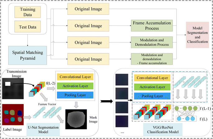
This paper proposes that various combinations of spatial pyramid matching model (SPM), M_D and FA not only enhance quality of image but also further improve the accuracy of heterogeneous classification in MTI within deep learning network models. It includes the design of experiments for collecting MTI of phantom, and the implementation of different combinations of SPM, M_D and FA to improve the quality and clarity of images. The multi-spectral fusion pseudo-color images obtained from U-Net semantic segmentation are then inputted VGG16/19 and ResNet50/101 networks for heterogeneous classification. Compared to the original images, all pre-processing methods effectively improve the accuracy of heterogeneous classification in VGG and ResNet network models. The framework of heterogeneous classification detection model in biological tissues is shown in Fig. 1.

Fig. 1 The overall classification model frame diagram.

2. Related method

2.1 Space pyramid matching model (SPM)

The SPM divides image into a spatial pyramid from the horizontal and vertical directions, divides image into uniform grids of different granularities according to different levels, then counts the frequency of visual words in each grid, and calculates the frequency of each grid. The visual vocabulary histogram of grid is obtained, and finally the histograms of each sub-region are weighted and connected to form an image representation.⁸⁶ Assuming the existence of two feature sets X and Y, these sets are divided into different scales l = 0 ,…, L, creating 4^l cells in the feature space. The number of matches between the two feature sets in each cell is calculated, and then the histogram vectors of visual features are established. H^l_X and H^l_Y represent the histogram features of X and Y under scale l, respectively. The similarity between the two feature sets is calculated using the histogram intersection function as shown in eqn (1). To improve the matching accuracy of images, it is necessary to densely partition images. However, due to computational complexity, this paper adopts a three-level partitioning method. Finally, SPM kernel function is used for matching, and the computation of spatial matching kernel function is shown in eqn (2).

2.2 Modulation-demodulation (M_D) and frame accumulation (FA) technology

During multi-spectral transmission imaging, two primary noise categories emerge: random noise (including dark current, photon, granular, and readout noise) and image noise (categorized as fixed and non-uniform). To mitigate random noise during imaging, we adjust the parameters of the excitation light source, which employs a sinusoidal waveform, to facilitate real-time transmission of the fundamental wave signal. This enhancement strategy improves the quality of multi-spectral images. The modulation process involves controlling selected parameters of the carrier signal using a baseband signal to create a modulation signal suitable for transmission. In the absence of noise, a multiplication filter is employed to demodulate the modulated signal in the frequency domain, yielding high-quality multi-spectral images. Specifically, our approach utilizes a sinusoidal signal as the carrier for the excitation light source. During modulation, we ensure that the camera operates within its linear range, steering clear of low-energy zones and saturation points, thereby preventing nonlinear image noise. Furthermore, we employ frame accumulation to suppress image noise by overlaying multiple frame images while maintaining image precision. This technique enhances both the signal-to-noise ratio (SNR) and grayscale resolution of the image. Notably, the improvement in SNR through frame accumulation correlates with the number of frames accumulated, as illustrated in eqn (3) and (4).where represents the sum of image noise of m frames images; σ²_n is the variance of image noise. Therefore, after accumulating m frame images, the SNR of accumulated image is m times of original single-frame image.

2.3 U-Net network

In medical image segmentation tasks, U-Net stands out as one of the most successful methods. Unlike fully convolutional networks (FCN), the pivotal distinctions in U-Net reside in its encoder and skip connection components. The network architecture of U-Net is fully symmetrical, mirroring similar structures on both sides. In the skip connection part, U-Net transfers features extracted by the encoder part to the decoder part fully, utilizing concatenation operations to merge features.⁸⁷ The schematic of U-Net is illustrated in Fig. 2. Initially, the encoder part acquires detailed and contour information of the image. Subsequently, the extracted features are relayed to the decoder part via the skip connection stage. Ultimately, the decoder part integrates features from multiple scales for feature restoration and enhancement. The pervasive adoption of U-Net in medical image segmentation is attributed to: (1) its remarkable capacity to yield satisfactory results with minimal training data. (2) The efficacy and robustness of its network structure.

Fig. 2 U-Net architecture model.

2.4 VGG network

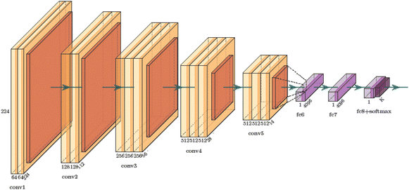
The VGG network architecture is shown in Fig. 3.⁸⁸ Its main characteristics are as follows: the convolutional layers employ convolutional kernels with uniform parameters to ensure consistency in the width and height of tensors between each convolutional layer. All pooling kernel parameters used in the pooling layer are identical, with a size of 2 × 2 and a stride of 2, aiming to halve the length and width of the tensor after the pooling operation and reduce the number of parameters. Instead of using large convolutional kernels, small convolutional kernels are stacked to achieve the same receptive field. For instance, two 3 × 3 convolutional kernels can replace a 5 × 5 convolutional kernel while maintaining the same receptive field, and similarly, three 3 × 3 convolutional kernels can substitute for a 7 × 7 convolutional kernel with an equivalent receptive field. Consequently, when the feature extraction effect is comparable, multiple small convolutional kernels possess fewer learning parameters compared to large convolutional kernels. This approach not only enhances model performance but also allows for the increase in network depth.

Fig. 3 VGG network structure.

2.5 ResNet network

ResNet is a type of deep residual network that effectively addresses issues like vanishing and exploding gradients.⁸⁹ It significantly boosts network performance as its depth increases. By modifying the model structure, identity mapping is incorporated on top of stacked network weight layers, thereby forming a residual structure. This innovation addresses the issue of network layer saturation and yields a superior model architecture. The comparison between traditional neural network units and residual network units is illustrated in Fig. 4. For the conventional neural network unit structure shown in Fig. 4a, assuming the input of a certain layer is x_l and its output is x_l+1, the gradient calculation formula is shown in eqn (5). In traditional networks, the data source for a given layer is solely derived from the preceding layer's network. When a neural network model consists of numerous traditional neural network structures stacked together, the propagation process entails both multiplication and addition operations during gradient calculation across layers. However, there is a notable enhancement when deep residual networks incorporate residual structures. The gradient calculation for these residual structures is depicted in eqn (6).

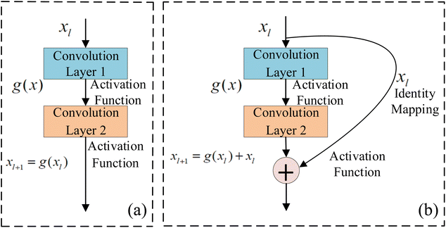Fig. 4 Traditional neural network and residual network unit structure (a) traditional convolutional network unit; (b) residual convolutional network unit.

3. Experiment

3.1 Experimental equipment

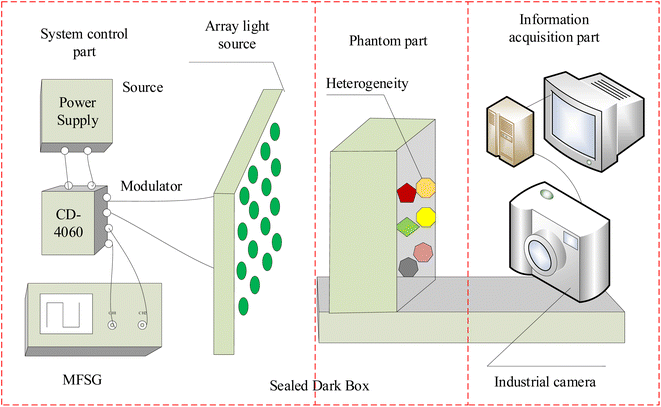
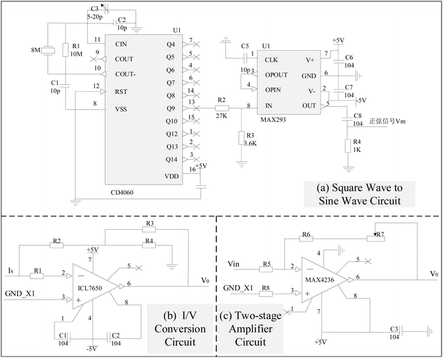
The experimental system device is shown in Fig. 5. The system mainly consists of a power supply, a modulator module, an array of LEDs with different wavelengths, an industrial camera, a computer, a black cloth and a phantom. The power supply is a programmable Direct Current (DC) stabilized power supply, and model is hspy-600. Considering the spectral window for biological applications, which spans from 650 nm to 950 nm, and acknowledging that combining various wavelengths can enhance the precision of heterogeneous detection, specific light sources are chosen: blue light centered at 435 nm, green light at 546 nm, red light at 700 nm, and near-infrared light at 860 nm. And the design of 4 × 4 LED array must ensure that its irradiation angle covers the entire phantom area, the LED light intensity range changes linearly. The industrial camera model is JHSM120Bf, with a frame rate/resolution of 29.4 fps@1280 × 960, a full transparent filter, exposure time ranging from 34.375 μs to 2252.765 ms, and spectral response from 390 nm to 1030 nm. The computer model is HuiPu, and usbVide software is used for MTI acquisition. Relative to other tissues, breast tissue has higher transmittance. Therefore, the phantom consists of a rectangular container made of highly translucent polymethyl methacrylate (PMMA) material. Overall scattering coefficient of the phantom is approximately 0.8 mm⁻¹, and the absorption coefficient is approximately 0.0044 mm⁻¹. The container is used to hold solutions of different concentrations of fat emulsion (2%, 3%, 5%) and heterogeneous block to simulate nodules in breast tissue. Among them, based on the distinct properties of breast tissue, namely its high transmissibility and tomographic distribution, potatoes, carrots, and pumpkins are utilized within the solution as heterogeneous elements to mimic breast cancer scenarios. And all variations in size fall within the dimensions of 0.7 cm × 0.7 cm × 1 cm. Heterogeneities are positioned at two-thirds of the phantom's width. The light source is situated directly in front of the phantom, with the camera placed at the opposite end, behind it.

Fig. 5 Experimental equipment diagram.

In order to obtain the sine wave with high stability and high precision, the sine wave conversion circuit of square wave is used to generate the required sine signal. Precise square-wave pulse signals can be generated by digital circuits and crystal oscillators. Because the frequency accuracy is only related to crystal oscillators, high precision signals can be obtained. The square wave signal can become the desired high-precision sine wave signal after low-pass filtering. The circuit schematic of the modulator module is displayed in Fig. 6, utilizing a square wave to sine wave conversion circuit to generate the necessary sine signal. Fig. 6a illustrates the circuit schematic for square wave to sine wave conversion, where CD4060 functions as a 14 bit binary serial counter/divider, producing a high-precision square wave signal of 3.5/4 Hz at its 13th pin (Q9 pin). The precision of its output signal is finely adjusted by C3. The square wave signal, subsequently attenuated through the gain control network R2 and R3, enters the low-pass filtering circuit, retaining only the fundamental frequency signal, thereby obtaining the sine wave signal at the identical frequency. Fig. 6b showcases the I/V conversion circuit, which employs the CMOS-based integrated chopper-stabilized zero-drift operational amplifier ICL7650 from Maxim Integrated. R1 serves as the input current-limiting protection resistor for the ICL7650. The smaller resistors R2, R3, and R4 form a T-network, replacing the traditional use of larger resistors to enhance gain stability and accuracy, while also reducing noise. In addition, since the photoelectric signal I_S four-channel, in order to reduce the interference between each other, the ground end of the four-channel signal should be temporarily separated from the power source. The I_S shown in the figure is the current signal reflecting the horizontal deflection angle, and its ground end is represented by GND_X1. The other three signals are connected in the same way, and in the PCB version, the four signal lines are isolated with envelope lines to reduce interference. And for effective amplification of microcurrent signals in the I/V conversion section, an inverted input type amplification circuit with a T-network is adopted, as shown in Fig. 6c, producing an amplified voltage signal with a phase opposite to the input current signal.

Fig. 6 Schematic diagram of sinusoidal forming signal generating circuit (a) schematic diagram of square wave to sine wave circuit; (b) schematic diagram of I/V conversion circuit; (c) schematic diagram of two-stage amplifier circuit.

3.2 Image acquisition

The original MTI are collected on the established experimental platform: fat emulsion solution + heterogeneity. The specific collection steps are as follows:

1. Set the parameters for the power supply, signal generator and industrial camera. Load different power loads based on the rated voltage and current values of different wavelengths LEDs. Use the signal generator to generate square wave signals of 4 Hz and 3.5 Hz. These signals are then modulated by the modulator module to produce sinusoidal waves with voltage bias above 0 V at the same frequency, as illustrated in Fig. 7. Based on the concentration of fat emulsion solution, set the gain (3, 7, and 10), exposure time (5 ms, 8 ms, and 10 ms) and sampling rate (45 frames per second) of camera accordingly. Acquire multi-spectral transmission phantom signal images adjusted by the amplification circuit.

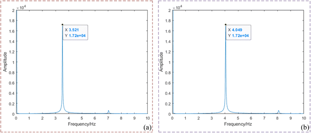Fig. 7 Modulation frequency diagram of molded signal (a) frequency domain diagram of 3.5 Hz; (b) frequency domain diagram of 4 Hz.

2. Adjust and fix the distance between the light source and the phantom, as well as between the phantom and the camera. During the adjustment of the distance between the light source and the phantom, ensure that the illumination angle formed by the LED array light source fully covers the entire area of the phantom. Simultaneously, continuously monitor the stability of the sine wave generated by the signal generator, ensuring that its intensity fluctuates in accordance with the sine wave. The distance between the phantom and the camera should be such that there is no occurrence of shadow noise within the imaging range. In this paper, a configuration is established where the LED array is positioned 25 centimeters away from the phantom, while maintaining a 45 centimeter separation between the phantom and the camera. The phantom includes six heterogeneities of varying sizes and thicknesses (2 potato blocks, 2 carrot blocks and 2 pumpkin blocks). The dimensions of heterogeneities are all within the range of 0.8 cm × 0.8 cm × 1 cm, and all heterogeneities are placed at 2/3 of the width of phantom.

3. Four types of LED arrays loaded with 4 Hz and 3.5 Hz sinusoidal signal wavelengths are individually irradiated to acquire the original MTI. The entire experiment is enclosed with a black cloth to eliminate external light interference. Each wavelength LED array illuminates five groups of phantoms, each containing different concentrations (specifically, 2 groups with a 2% concentration fat emulsion solution, 2 groups with a 3% concentration fat emulsion solution, and 1 group with a 5% concentration fat emulsion solution). In total, 60 sets of original and modulated image data are collected for all wavelengths, with each set comprising 1200 frames of images, amounting to a grand total of 72 000 frames of MTI.

3.3 Image preprocessing

The acquired MTI are M_D, FA, modulation and demodulation-frame accumulation (M_D-FA) and scattering coefficient correction respectively. The specific processing steps are as follows:

1. M_D processing of images. Perform fast Fourier transform (FFT) on all acquired modulated images to obtain the frequency coordinates of images loaded with sine signals, as shown in Fig. 8. Fig. 8a corresponds to the frequency domain coordinates at 4 Hz, and Fig. 8b corresponds to the frequency domain coordinates at 3.5 Hz. Demodulate multi-spectral images for all wavelengths based on the frequency domain coordinates, resulting in a total of 48 000 frames of M_D images at different frequencies, with each wavelength comprising 6000 frames.

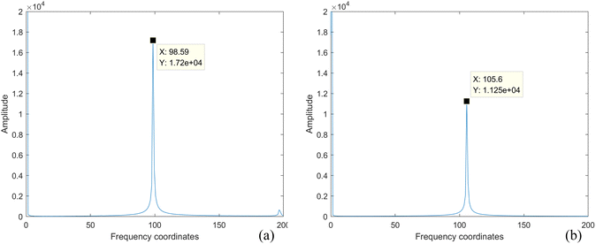Fig. 8 4 Hz and 3.5 Hz frequency domain coordinate diagram (a) frequency domain coordinate diagram corresponding to 4 Hz; (b) frequency domain coordinate diagram corresponding to 3.5 Hz.

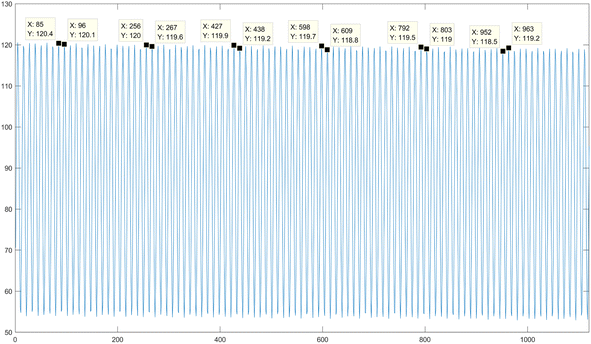
2. FA processing of images. Taking the accumulation process of a single group of multi-spectral image frames at the near-infrared wavelength as an example, the average gray value of the 1200 frames of low-light level images is calculated, as illustrated in Fig. 9. From the figure, it can be clearly observed that a single cycle of the sine signal consists of 12 frames of images. FA averaging processing is sequentially performed on every 12 frames of images to obtain FA images for all wavelengths. As a result, a total of 2000 frames of FA images are obtained, with each wavelength contributing 500 frames.

Fig. 9 Period diagram of near infrared light sinusoidal signal.

3. M_D-FA processing of images. Similarly, the images demodulated at different frequencies are subjected to FA averaging processing for every 12 frames of images within a single sine signal cycle. This process results in M_D-FA images for all wavelengths, totaling 4000 frames of images, with each wavelength comprising 500 frames.

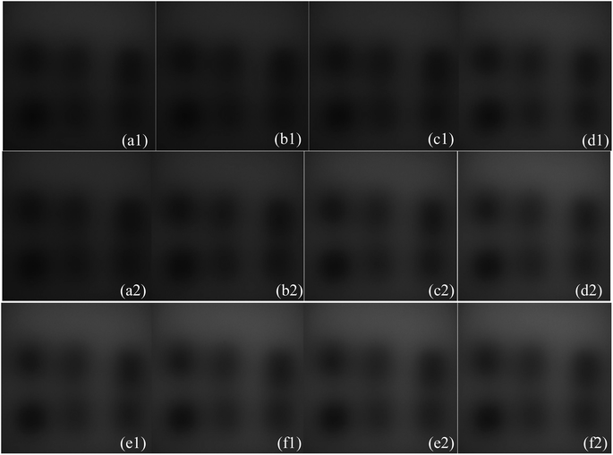
4. Image scattering coefficient correction. Before capturing images, obtain the ground truth images of all wavelengths for the heterogeneities, as shown in Fig. 10. Utilize a SPM to statistically analyze different spatial feature points in images to calculate the matching degree between each set of original images, FA images, M_D images, M_D-FA images and their corresponding ground truth images for different wavelengths. Based on the obtained matching coefficients, proportionally adjust the grayscale values of the images in a sequential manner. Fig. 11 shows the scattering coefficient before and after correction.

Fig. 10 Ground truth image of 4 wavelengths (a) ground truth image of green light wavelength; (b) ground truth image of blue light wavelength; (c) ground truth image of red light wavelength; (d) ground truth image of near-infrared light.

Fig. 11 Preprocessed images before and after scattering coefficient correction (a) original images; (b) FA image; (c) 4 Hz M_D images; (d) 3.5 Hz M_D images; (e) 4 Hz M_D-FA images; (f) 3.5 Hz M_D-FA images. Note: 1 means before scattering coefficient correction, 2 means after scattering coefficient correction.

3.4 Image U-Net network semantic segmentation

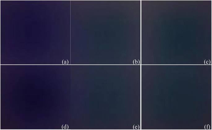
1. MTI U-Net semantic segmentation. Firstly, to promote the potential of multi-spectral transmission images in breast cancer detection, the four-wavelength original MTI are combined in the order of blue light, green light, red light, and near-infrared light, according to the proportions of an RGB color image, resulting in a pseudo-color image as shown in Fig. 12a. Then, input the obtained pseudo-color image into the U-Net semantic segmentation network model for training, obtaining semantic segmentation annotations for the six heterogeneities in pseudo-color image, as shown in Fig. 12b. Finally, acquire the original segmentation images of six heterogeneities through mask processing, as shown in Fig. 12c.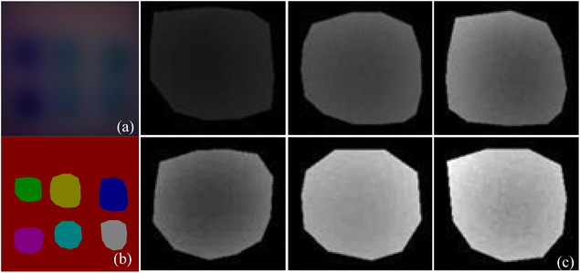

Fig. 12 U-Net network semantic segmentation process (a) original pseudo-color image; (b) semantic segmentation map of six different heterogeneities; (c) mask segmentation of original image.

2. Obtaining pseudo-color images. Based on the proportional relationships of RGB primary colors in color image, recombine segmentation images to obtain original pseudo-color images, M_D pseudo-color images, FA pseudo-color images and M_D-FA pseudo-color images. The four-wavelength images are combined in the order of blue, green, red and near-infrared light, with each combination comprising every 3 wavelengths, resulting in a total of A³₄ = 24 combinations. This yields 57 600 frames of original pseudo-color images, 115 200 frames of M_D pseudo-color images, 4800 frames of FA pseudo-color images, and 9600 frames of M_D-FA pseudo-color images. The obtained pseudo-color images are divided successively according to the mask region, and the 6 different heterogeneities are shown in Fig. 13.

Fig. 13 Six types of heterogeneous pseudo-color images after U-Net network segmentation (a) pseudo-color image of heterogeneity 1; (b) pseudo-color image of heterogeneity 2; (c) pseudo-color image of heterogeneity 3; (d) pseudo-color image of heterogeneity 4; (e) pseudo-color image of heterogeneity 5; (f) pseudo-color image of heterogeneity 6.

3.5 Heterogeneous detection

3.5.1. Dataset creation. Six categories of pseudo-color images after multi-spectral semantic segmentation before and after scattering correction are made into original dataset a(a1 and a2), FA dataset b(b1 and b2), 4 Hz M_D dataset c(c1 and c2), 3.5 Hz M_D dataset d(d1 and d2), 4 Hz M_D-FA dataset e(e1 and e2) and 3.5 Hz M_D-FA f(e1 and e2). The images in dataset are divided into 6 categories: potato block 1, potato block 2, carrot block 1, carrot block 2, pumpkin block 1 and pumpkin block 2. And data sets a, b, c, d, e and f are randomly divided into training sets, verification sets and test sets using random functions, and the ratio is set to 6 : 1 : 3 according to the traditional partition ratio in the field of machine learning.

3.5.2. Model training. VGG16, VGG19, ResNet50 and ResNet101 networks are selected as the heterogeneous classification models. The datasets a, b, c, d, e and f are input into the VGG and ResNet networks for training according to the specified ratios. The best model for different datasets is established by comparing the accuracy, precision, recall and F-score of models. For VGG networks, the batch size is set to 32, Adam optimizer is used, the initial learning rate is set to 0.0001, the number of iterations is set to 30, and the training step size is set to 100. For ResNet networks, the batch size is set to 16, Adam optimizer is also used, the initial learning rate is set to 0.0001, the number of iterations is set to 80, and the training step size is also set to 100.

3.5.3. Data visualization. The visualization of the first 36 channel feature maps before the convolutional layers of VGG/ResNet network is shown in Fig. 14. In Fig. 14, the lower layers of the network, such as conv1_2, primarily extract color and edge features from the pseudo-color images of heterogeneities. The middle layers of the network, such as conv3_3, mainly capture simple texture features of the heterogeneities. Meanwhile, the higher layers of the network, like conv5_3, predominantly extract abstract features of the heterogeneities at a finer level.

Fig. 14 Original image and convolutional feature maps (a) pseudo-color image of heterogeneous entities; (b) feature map of conv1_2; (c) feature map of conv2_2; (d) feature map of conv3_3; (e) feature map of conv4_3; (f) feature map of conv5_3.

4. Results and analysis

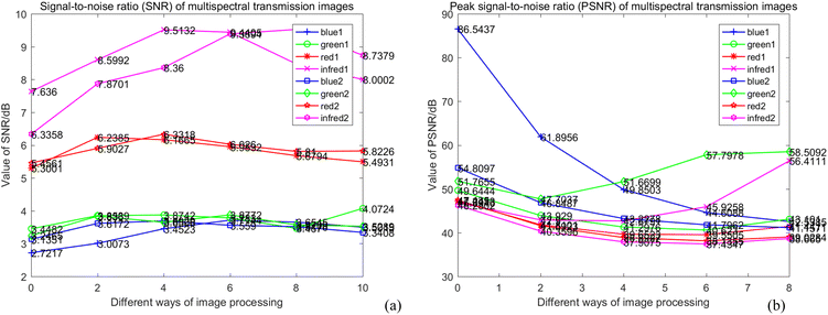
After M_D, FA and scattering correction, the quality of MTI is improved significantly. Among them, the gray level of the image is stretched, the SNR is gradually increased. In deep learning networks (VGG and ResNet), pseudo-color images with different wavelength fusion can effectively detect and classify heterogeneities.

(1) M_D, FA and scatter correction significantly improve the quality of images. To clearly demonstrate the changes in image quality before and after preprocessing, the SNR and Peak Signal-to-Noise Ratio (PSNR) are calculated, as shown in eqn (7)–(9), and the results are shown in Table 2 and Fig. 15. A higher SNR indicates better image quality, manifested in clearer imaging of the tissues needed. A positive PSNR value indicates a significant increase in the grayscale levels of image after preprocessing, which is beneficial for the classification of heterogeneities within the image.

where K(i,j) represents ground truth image; f(i,j) represents the pixel value in image; represents the average value of image pixels; mn represents the size of image; I(i,j) represents processed image. From Table 2, it can be observed that: ① the SNR of all wavelength images obtained by different preprocessing methods has a certain improvement compared with original image. (a) Prior to image scattering coefficient correction, the SNR of the 3.5 Hz M_D image in the blue wavelength experiences the most significant increase, which is 36.5%. (b) After correction of image scattering coefficients, the highest SNR improvement is observed in the near-infrared light wavelength with a 4 Hz M_D image, reaching 50.34%. ② The SNR results before and after the correction of scattering coefficients for different wavelength images are shown in Fig. 15a. (a) In the blue light wavelength, the SNR of 3.5 Hz M_D image and the 4 Hz/3.5 Hz M_D-FA image are lower than the image before scattering correction, while other preprocessing methods are higher than the SNR before scattering correction. (b) In the green light wavelength, except for the SNR of 3.5 Hz M_D and 4 Hz M_D-FA image, which are higher than before scattering correction, other preprocessing methods are lower than the SNR before scattering correction. (c) In the red light wavelength, except for FA image, the SNR of other image preprocessing methods are higher than before scattering correction. (d) In the near-infrared light wavelength, except for the 3.5 Hz M_D image, the SNR of other image preprocessing methods are higher than before scattering correction. ③ The PSNR of images at all wavelengths under different preprocessing methods is positive. As shown in Fig. 15b, the scattering coefficients of FA and 4 Hz/3.5 Hz M_D images at the blue wavelength, 3.5 Hz M_D images and 4 Hz M_D and FA images at the green wavelength before and after correction are significantly different, and the scattering coefficients of other preprocessing methods change little.

Table 2 Comparison of SNR and PSNR for different wavelength images under different preprocessing methods

Image/preprocessing			Original	FA	4 Hz M_D	3.5 Hz M_D	4 Hz M_D-FA	3.5 Hz M_D-FA
Non-scattering correction	Blue1	SNR1	2.7217	—	—	—	—	—
		SNR2	—	3.0073	3.4523	3.7144	3.6545	3.5015
		PSNR	—	86.5437	61.8956	49.8503	44.6088	42.5385
	Green1	SNR1	3.4482	—	—	—	—	—
		SNR2	—	3.8539	3.8742	3.7830	3.4670	4.0724
		PSNR	—	49.6444	43.9290	41.2976	40.6230	43.1010
	Red1	SNR1	5.3001	—	—	—	—	—
		SNR2	—	6.2385	6.1665	5.9532	5.6794	5.4931
		PSNR	—	47.2423	41.8101	39.6523	39.5505	41.4411
	Infra1	SNR1	7.6360	—	—	—	—	—
		SNR2	—	8.5992	9.5132	9.4405	8.4726	8.0002
		PSNR	—	46.8916	42.9000	42.6791	45.9258	56.4111
Scattering correction	Blue2	SNR1	3.1351	—	—	—	—	—
		SNR2	—	3.6172	3.6929	3.5590	3.5176	3.3408
		PSNR	—	54.8097	46.8487	43.2278	41.7962	41.1571
	Green2	SNR1	3.2465	—	—	—	—	—
		SNR2	—	3.8360	3.6506	3.8772	3.5709	3.5289
		PSNR	—	51.7655	47.7037	51.6699	57.7978	58.5092
	Red2	SNR1	5.4561	—	—	—	—	—
		SNR2	—	5.9027	6.3318	6.0260	5.8100	5.8226
		PSNR	—	47.4350	41.5923	38.8927	38.1355	39.0284
	Infra2	SNR1	6.3358	—	—	—	—	—
		SNR2	—	7.8701	8.3600	9.3894	9.5254	8.7379
		PSNR	—	46.2502	40.3596	37.9075	37.4347	38.6650

---

Fig. 15 Comparison of SNR and PSNR under different image preprocessing methods before and after scattering coefficient correction (a) comparison of SNR under different image preprocessing methods; (b) PSNR comparison diagram under different image preprocessing methods.

(2) Both VGG and ResNet network models can effectively detect heterogeneity in MTI. To comprehensively measure the performance of model, this paper takes accuracy, precision, recall and F-score as evaluation indicators. True Positive (TP) represents the positive sample predicted by the model, True Negative (TN) represents the negative sample predicted to be negative, False Positive (FP) represents the negative sample predicted to be positive, and False Negative (FN) represents a positive sample that is predicted to be negative. Recall rate and precision rate are a pair of contradictory quantities, the recall rate is relatively low when the precision rate is high. When the recall rate is relatively high, the precision rate is relatively low, so when the recall rate and the precision rate are relatively high, it means that the classification effect of this network is better. F-score is used to measure both recall and precision attributes. The definition equations for calculating the above evaluation indicators through the confusion matrix is as follows:

The VGG16 and VGG19 models have both demonstrated effective classification detection of heterogeneities in MTI. Pseudo-color images fused with different wavelengths are trained in the VGG16 and VGG19 networks respectively to achieve the classification of heterogeneity in multi-spectral images. The results are shown in Table 3. From Tables 3 and it can be observed that: ① compared to original images, all image preprocessing methods significantly enhance the accuracy of heterogeneous classification. The widest increase in heterogeneous classification accuracy is achieved with the 3.5 Hz M_D images without scatter correction, reaching 18.53%. ② Both before and after scatter correction, the overall classification accuracy of the VGG19 network model surpasses that of VGG16. ③ After scatter correction, the overall heterogeneous classification accuracy of both VGG16 and VGG19 network models increases compared to before scatter correction, and this accuracy is also higher than before scatter correction across all preprocessing methods. ④ Before scatter correction, the highest classification accuracy for heterogeneities in the 3.5 Hz M_D images is attained in the VGG16 network model, reaching 91.28%. In contrast, the VGG19 network model achieves its highest classification accuracy with the 3.5 Hz M_D-FA images, reaching 91.99%. ⑤ After scatter correction, both VGG16 and VGG19 network models attain their peak classification accuracy for heterogeneities in the 3.5 Hz M_D-FA images, specifically 94.93% and 95.47%, respectively.

Table 3 Classification results of 6 different heterogeneities by VGG16/19 network model

Data type		VGG16				VGG19
		Accuracy%	Precision%	Recall%	F 1-Score	Accuracy%	Precision%	Recall%	F 1-Score
Non-scattering correction	Original	77.01	78.73	77.40	0.7679	83.62	84.26	83.56	0.8386
	FA	81.79	82.89	81.52	0.8196	84.13	84.54	84.13	0.8429
	4 Hz M_D	88.33	89.27	88.33	0.8805	89.05	89.54	89.05	0.8871
	3.5 Hz M_D	91.28	92.06	91.28	0.9079	89.52	90.26	89.52	0.8925
	4 Hz M_D-FA	90.58	91.30	90.57	0.9005	91.41	92.01	91.41	0.9095
	3.5 Hz M_D-FA	88.57	89.46	88.57	0.8827	91.99	92.96	91.99	0.9161
Scattering correction	Original	83.72	84.57	83.50	0.8374	84.84	85.41	84.71	0.8500
	FA	84.64	84.98	84.85	0.8477	85.14	85.40	85.29	0.8532
	4 Hz M_D	91.30	92.22	91.30	0.9080	95.00	95.25	95.00	0.9489
	3.5 Hz M_D	92.18	93.69	92.18	0.9191	95.07	95.46	95.07	0.9500
	4 Hz M_D-FA	94.53	94.59	94.53	0.9442	95.27	95.43	95.27	0.9516
	3.5 Hz M_D-FA	94.93	95.37	94.93	0.9487	95.47	95.66	95.47	0.953

---

The ResNet50 and ResNet101 models further improved the accuracy of heterogeneous classification in MTI, as shown in Table 4. From Table 4, it can be observed that: ① compared to original images, all image preprocessing methods effectively improved the accuracy of heterogeneous classification. The widest increase in heterogeneous classification accuracy is achieved with the 3.5 Hz M_D-FA images with scatter correction, reaching 10.21%. Furthermore, both before and after scatter correction, as the preprocessing methods are progressively applied, the classification accuracy of the ResNet network models also gradually increases. ② Before and after scatter correction, the overall classification accuracy of ResNet101 network model is higher than that of the ResNet50 network model, but the increase in accuracy with different preprocessing methods is relatively small. ③ After scatter correction, the overall heterogeneous classification accuracy of both ResNet50 and ResNet101 network models surpasses that before scatter correction, and this accuracy is also higher than before scatter correction under all preprocessing methods. ④ Before and after scatter correction, the ResNet network models achieve the highest classification accuracy of heterogeneities in the 3.5 Hz M_D-FA images. Specifically, the accuracies are 95.33% and 95.13% before scatter correction, and 98.06% and 98.47% after scatter correction for ResNet50 and ResNet101, respectively.

Table 4 Classification results of 6 different heterogeneities by ResNet50/101 network model

Data type		ResNet50				ResNet101
		Accuracy%	Precision%	Recall%	F 1-Score	Accuracy%	Precision%	Recall%	F 1-Score
Non-scattering correction	Original	88.57	89.46	88.57	0.8827	88.69	89.20	8869	0.8839
	FA	88.75	89.51	88.75	0.8843	88.87	89.24	88.87	0.8854
	4 Hz M_D	93.88	94.21	93.88	0.9393	94.63	95.01	94.63	0.9464
	3.5 Hz M_D	94.76	94.93	94.76	0.9473	94.89	95.20	94.89	0.9489
	4 Hz M_D-FA	96.13	96.27	96.13	0.9614	96.27	96.37	96.27	0.9627
	3.5 Hz M_D-FA	95.13	95.49	95.13	0.9505	95.33	95.72	95.33	0.9527
Scattering correction	Original	89.11	90.34	89.11	0.8881	89.35	90.07	89.35	0.8911
	FA	89.35	89.90	89.35	0.8901	89.58	90.15	89.58	0.8927
	4 Hz M_D	95.13	95.49	95.13	0.9505	95.33	95.72	95.33	0.9527
	3.5 Hz M_D	96.47	96.52	96.47	0.9647	96.93	97.00	96.93	0.9694
	4 Hz M_D-FA	97.57	97.66	97.57	0.9757	97.92	97.96	97.92	0.9791
	3.5 Hz M_D-FA	98.06	98.06	98.06	0.9805	98.47	0.9849	98.47	0.9847

---

(3) Analysis and discussion of experimental results. (a) Based on the analysis of experimental results, different combinations of SPM, M_D, and FA techniques were employed to varying degrees to enhance the quality and clarity of images. Compared with the original images, all the image preprocessing methods effectively improved the classification accuracy of heterogeneities in both VGG and ResNet models. Notably, the overall classification accuracy of the ResNet model was higher than that of the VGG model. Specifically, the accuracy of heterogeneous classification for 3.5 Hz M_D images with un-scattered correction increased by the widest margin, reaching 18.53% in the VGG model. In contrast, 3.5 Hz M_D-FA images with scattering correction exhibited the largest increase in heterogeneous classification accuracy, reaching 10.21% in the ResNet model. Moreover, as can be seen from Table 5, the p-values are all less than 0.001, strongly indicating that the different models after correction have significantly improved performance compared to those before correction. Additionally, the F-values are all above 150, further confirming that the differences between the models before and after correction are much larger in terms of inter-group variance than intra-group variance, thereby further reinforcing the significance of the model performance improvements. Despite these significant advantages, the study faces limitations, including the complexity and computational overhead of preprocessing steps, which may hinder real-time applicability. Furthermore, the techniques' sensitivity to specific parameters necessitates further experimentation and tuning. Lastly, the evaluation environment was limited to phantom-based experiments, which may not fully capture the nuances and complexities of real-world breast tumor imaging, highlighting the need for further validation in clinical settings with a larger and more diverse patient population to confirm the generalizability of the results.

Table 5 Analysis of variance (ANOVA) before and after scattering correction for different models

Model	F-Value	p-Value
VGG16	151.28	<0.001
VGG19	155.61	<0.001
ResNet50	155.71	<0.001
ResNet50	157.81	<0.001

---

5. Discussions

In our study, we utilized a combination of SPM, M_D, and frame accumulation FA techniques to significantly enhance the quality and clarity of MTI, thereby facilitating more accurate heterogeneous classification. These preprocessing methods effectively reduced noise, improved contrast, and enhanced image details. Furthermore, we employed deep learning models, particularly VGG16/19 and ResNet50/101, which have proven effective in image recognition and classification tasks due to their ability to learn complex patterns and features from large datasets. The models captured subtle differences between heterogeneous regions in the MTI, resulting in improved classification performance. Additionally, we introduced multi-spectral fusion pseudo-color images obtained through U-Net semantic segmentation, providing additional information for the classification task by leveraging a richer set of features from images of different wavelengths. Specifically, we observed that 3.5 Hz M_D images without scatter correction significantly increased heterogeneous classification accuracy, potentially due to the effectiveness of the M_D technique in feature extraction and the model's ability to focus on raw signals without distraction from scattered light. The VGG19 model demonstrated higher overall classification accuracy compared to VGG16, likely due to its increased depth and complexity, allowing it to learn more nuanced features. Scatter correction further improved classification accuracy by reducing noise and artifacts caused by scattered light. Ultimately, the highest classification accuracy was achieved with 3.5 Hz M_D-FA images in both VGG and ResNet models, highlighting the combined benefits of M_D and FA techniques in extracting relevant features and enhancing the signal-to-noise ratio, respectively.

In the context of enhancing MTI for heterogeneous classification, the algorithm complexity of the proposed method involves considering the individual complexities of SPM, M_D, and FA. SPM scales as O(N^2*L) with image size and pyramid levels, M_D approximates as O(N^2*P) with potential for parallel processing, and FA scales as O(N^2*K). While these preprocessing steps add computational overhead, they significantly improve image quality and feature extraction, leading to high classification accuracy (95.47% with VGG19 and 98.47% with ResNet101). The trade-offs between preprocessing time and accuracy improvements justify the computational cost, particularly in clinical applications requiring high accuracy. Future work aims to optimize the preprocessing pipeline for reduced computation time while maintaining accuracy.

The proposed method significantly enhances heterogeneous classification accuracy using MTI within deep learning models, but it faces challenges in transitioning to clinical applications. Notably, the use of phantoms in experiments may not fully capture the complexity and variability of real-world patient data, which includes diverse anatomical structures, tissue types, and disease states that affect light absorption and scattering. Therefore, additional validation using a larger and more diverse set of clinical data is essential to ensure the robustness and generalizability of the method in a clinical setting.

The proposed method, leveraging MTI within deep learning models, significantly improves heterogeneous classification accuracy. However, it faces challenges in algorithmic complexity and integration into clinical workflows. The preprocessing steps, including SPM, M_D, and FA, increase computational overhead, while the deep learning models (VGG16/19, ResNet50/101) demand substantial computational resources. To address these limitations, future work should focus on optimizing the preprocessing pipeline for efficiency, exploring integration into clinical workflows through user-friendly tools, and reducing the computational requirements of the deep learning models using techniques such as model compression or distillation. These efforts are crucial to ensure the robustness, generalizability, and clinical applicability of the proposed method.

6. Conclusion

In this study, we address the challenges associated with identifying heterogeneities in MTI of biological tissues, which are often obscured by absorption and scattering effects during transmission. The originality of our work lies in the innovative combination of SPM, M_D, and FA techniques to enhance image quality and, consequently, improve the accuracy of heterogeneous classification within DLNM. Firstly, we designed experiments to collect MTI of phantoms, which simulate breast tissue, leveraging the strong transmissibility and tomographic distribution characteristics of breast tissue. Potatoes, carrots, and pumpkins were chosen as heterogeneous models to represent different tissue densities and scattering properties, thereby mimicking breast cancer conditions. While this phantom-based approach may be influenced by other undisclosed factors, it provides a valuable initial framework for detecting heterogeneity within breast tissue. Secondly, we applied a multi-faceted preprocessing approach that involved separately processing the images through various combinations of SPM, M_D, and FA techniques. These combinations significantly improved the quality of the images, facilitating the extraction of heterogeneous feature information from multi-spectral images. By enhancing the image quality, we made it easier for DLNM to identify and classify the heterogeneities. Finally, we utilized U-Net semantic segmentation to generate multi-spectral fusion pseudo-color images, which were then inputted into VGG16/19 and ResNet50/101 networks for heterogeneous classification. The results demonstrated that all preprocessing methods effectively improved the classification accuracy of heterogeneities in both VGG and ResNet network models compared to the original images. Notably, after scatter correction, the images processed with 3.5 Hz M_D-FA achieved the highest classification accuracy of heterogeneities, reaching 95.47% in the VGG19 model and 98.47% in the ResNet101 model.

The significance of our study lies in its ability to overcome the limitations of traditional MTI techniques, which often struggle with image quality and heterogeneous classification accuracy. By incorporating SPM, M_D, and FA techniques, we have demonstrated a substantial improvement in both areas. This advancement not only enhances the clinical application of MTI technology in breast tumor screening but also opens up new possibilities for studying and identifying heterogeneities in other biological tissues. Moreover, existing clinical examination techniques often fall short in meeting all the characteristics required for effective breast tumor detection simultaneously, including regularity, non-radiation, cost-effectiveness, convenience, and ease of implementation. Our study represents an innovative attempt in this field by proposing the utilization of optical multi-spectral transmission imaging for breast cancer detection. Our approach aims to address these challenges and provide a comprehensive solution that meets the diverse needs of breast tumor screening. While our study has shown promising results, it is not without limitations. The preprocessing steps are complex and sensitive to specific parameters, which may hinder real-time applicability and require further experimentation. Additionally, our evaluation was limited to phantom-based experiments, and further validation in clinical settings with a larger, diverse patient population is necessary to strengthen the clinical relevance of our findings. Despite this, this study presents a valuable concept for detecting heterogeneity within breast tissue and offers a foundation for future research in this area.

Ethical statement

For our research involving the use of phantoms, ethical approval is not required as it does not involve the use of humans or animals.

Author contributions

Fulong Liu: conceived and designed the experiments, performed the experiments, analyzed the data, wrote the paper. Gang Li: contributed reagents, materials, and analysis tools, reviewed and edited the manuscript. Junqi Wang: asssisted with data analysis, provided critical feedback, and helped revise the manuscript.

Conflicts of interest

The authors declare that they have no conflict of interest.

Acknowledgements

This work was supported by the Fundamental Research Funds for the Central Universities of Jiangsu Province (Natural Science), with the project number of 24KJB310022. Thank you for the equipment provided by the State Key Laboratory of Precision Measurement Technology and Instruments of Tianjin University.

References

1. W. Y. Hu, D. D. Xu and N. L. Li, Cancer Control, 2023, 30 DOI:10.1177/10732748231209193.
2. A. N. Giaquinto, H. Sung and K. D. Miller, Ca-Cancer J. Clin., 2023, 72, 524–541.
3. S. Hofvind, N. Moshina and Å. S. Holen, Radiology, 2021, 300, 66–76.
4. D. Coronado-Gutierrez, G. Santamaria and S. Ganau, Ultrasound Med. Biol., 2019, 45(11), 2932–2941.
5. S. Taralli, M. Lorusso and E. Perrone, Cancers, 2023, 15, 908.
6. A. Alikhassi, X. Li and F. Au, Breast Cancer Res. Treat., 2023, 321–334.
7. V. Ntziachristos and B. Chance, Breast Cancer Res., 2000, 3(1), 41–46.
8. X. Yang, G. Li and L. Lin, Conference on Optics in Health Care and Biomedical Optics VII, 2016.
9. F. L. Jiang, P. C. Liu and X. D. Zhou, Pattern Recognit. Lett., 2019, 128, 30–37.
10. R. Hou, Y. H. Zhao and S. M. Tian, J. Vis. Commun. Image Represent., 2019, 64.
11. H. Y. Tang, D. Kim and G. Li, Opt. Lett., 2012, 37(8), 1361–1363.
12. X. Yang, Y. J. Hu and G. Li, Rev. Sci. Instrum., 2016, 87(11), 115106.
13. Y. J. Hu, X. Yang and M. J. Wang, J. Mod. Opt., 2016, 63, 1539–1543.
14. E. Verburg, C. H. van Gils and B. H. M. van der Velden, Radiology, 2022, 302(1), 29–36.
15. D. N. F. P. Mohamad, S. Mashohor and R. Mahmud, Artif Intell Rev., 2023, 56(12), 15271–15300.
16. O. B. Naeem, Y. Saleem and M. U. G. Khan, Arch. Comput. Methods Eng., 2024, 2431–2449.
17. K. J. Tsai, M. C. Chou and H. M. Li, Sensors, 2022, 22, 1160.
18. M. M. Abdelsamea, M. H. Mohamed and M. Bamatraf, Cancer Inf., 2019, 18 DOI:10.1177/1176935119857570.
19. N. Rane, J. Sunny and R. Kanade, Int. J. Eng. Res. Sci. Technol., 2020, 9, 576–580.
20. M. M. Srikantamurthy, V. Rallabandi, D. B. Dudekula, S. Natarajan and J. Park, BMC Med. Imaging, 2023, 23, 1–15.
21. H. Li, S. Zhuang, D.-a. Li and J. Zhao, Biomed. Signal Process., 2019, 51, 347–354.
22. Y. Mo, C. Han and Y. Liu, IEEE Trans. Med. Imaging, 2023, 1696–1706.
23. H. Liu, Y. Chen and Y. Zhang, Eur. Radiol., 2021, 31, 5902–5912.
24. G. Ayana, K. Dese and S.-W. Choe, Cancers, 2021, 13, 738.
25. G. Ayana, J. Park and J.-W. Jeong, Diagnostics, 2022, 12, 135.
26. Y. Zhang, J.-H. Chen and Y. Lin, Eur. Radiol., 2021, 31, 2559–2567.
27. M. Jiang, D. Zhang and S.-C. Tang, Eur. Radiol., 2021, 31, 3673–3682.
28. H. Li, D. Chen and W. H. Nailon, IEEE Trans. Med. Imaging, 2021, 41, 3–13.
29. S. Xu, E. Adeli and J.-Z. Cheng, Int. J. Imaging Syst. Technol., 2020, 30, 1095–1107.
30. K. Sun, Y. Xin and Y. Ma, J. Intell. Fuzzy Syst., 2022, 42, 4205–4220.
31. C. Xu, Y. Qi and Y. Wang, Biomed. Signal Process., 2022, 71, 103178.
32. N. R. Rajalakshmi, R. Vidhyapriya and N. Elango, Int. J. Imaging Syst. Technol., 2021, 31, 59–71.
33. Y. Lei, X. He and J. Yao, Med. Phys., 2021, 48, 204–214.
34. S. Hussain, X. Xi and I. Ullah, Comput. Biol. Med., 2022, 149, 105995.
35. L. Zhu, R. Chen and H. Fu, Proceedings, PartVI 23, Springer, Lima, Peru, October 4–8, 2020, pp. 160–170.
36. G. Chen, Y. Dai and J. Zhang, Comput. Methods Programs Biomed., 2022, 225, 107086.
37. V. K. Singh, M. Abdel-Nasser and F. Akram, Expert Syst. Appl., 2020, 162, 113870.
38. J. Xing, Z. Li and B. Wang, IEEE/ACM Trans. Comput. Biol. Bioinf., 2020, 18, 2555–2565.
39. M. Byra, P. Jarosik and K. Dobruch-Sobczak, arXiv, 2020, preprint, arXiv:200110061,  DOI:10.48550/arXiv.2001.10061.
40. J. Li, Q. Zheng and M. Li, in Medical Image Computing and Computer Assisted Intervention-MICCAI 2022: 25th International Conference, Singapore, September 18-22, 2022, Proceedings, Part IV, Springer, 2022, pp. 391–400.
41. R. Huang, Z. Xu and Y. Xie, Expert Syst. Appl., 2023, 119962.
42. S. Wang, K. Sun and L. Wang, IEEE Trans Neural Netw Learn Syst., 2021, 1788–1800.
43. T. Lv and X. Pan, IEEE Trans Neural Netw Learn Syst., 2021, 2443–2457.
44. B. Gecer, S. Aksoy and E. Mercan, Pattern Recognit., 2018, 84, 345–356.
45. Z. Guo, H. Liu and H. Ni, Sci. Rep., 2022, 9, 882.
46. J. X. Wang, Y. J. Zheng and J. Ma, Med. Image Anal., 2022, 83, 104446.
47. H. Li, D. Chen and H. William, IEEE Trans. Med. Imaging, 2022, 41(1), 3–13.
48. Y. Wang, Z. Z. Wang and Y. Q. Feng, IEEE Trans. Med. Imaging, 2022, 41(3), 559–570.
49. Y. Luo, Q. Huang and X. Li, Pattern Recognit., 2022, 108603.
50. Z. He, M. W. Lin and Z. S. Xu, Inf. Sci., 2022, 608, 1093–1112.
51. W. C. Ding, J. Wang and W. J. Zhou, IEEE J Biomed Health Inform., 2022, 26(9), 4474–4485.
52. Y. F. Yang, Z. J. Liu and J. Huang, Theranostics, 2023, 13(4), 1342–1354.
53. T. T. Zheng, F. Lin and X. L. Li, Eclinicalmedicine, 2023, 58, 101899.
54. Y. Z. Luo, Q. H. Huang and L. Z. Liu, Pattern Recognit., 2023, 1793–6381.
55. S. H. Diao, W. R. Luo and J. X. Hou, IEEE J Biomed Health Inform., 2023, 27(3), 1535–1545.
56. J. Wu, Z. Xu, L. Shang, Z. Wang, Z. H. Wang, S. W. Zhou, H. Shang and J. H. Yin, Opt. Lasers Eng., 2023, 168, 1.1–1.8.
57. S. Kumbhare, A. B. Kathole and S. Shinde, Biomed. Signal Process., 2023, 86, 105080.
58. K. Atrey, B. K. Singh, N. K. Bodhey and R. B. Pachori, Biomed. Signal Process., 2023, 86, 104919.
59. S. Almutairi, S. Manimurugan, B. G. Kim, M. M. Aborokbah and C. Narmatha, Appl. Soft Comput., 2023, 110292.
60. A. Sahu, S. Meher and P. K. Das, Biomed. Signal Process., 2024, 105377.
61. P. Xiao, Z. Qin and D. J. Chen, IEEE Internet Things J., 2023, 10(11), 9878–9891.
62. T. Viriyasaranon, S. M. Woo and J. H. Choi, IEEE J Biomed Health Inform., 2023, 27(4), 2003–2014.
63. R. Ding, X. Zhou, D. Tan, Y. Su, C. Jiang, G. Yu and C. Zheng, Complex Intell. Syst., 2024, 10(3), 4571–4587.
64. T. Mahmood, T. Saba, A. Rehman and S. Alamrifaten, Expert Syst. Appl., 2024, 249, 123747.
65. K. Jabeen, M. A. Khan and R. Damasevicius, Eng. Appl. Artif. Intell., 2024, 137.
66. L. L. Liu, Y. Wang and P. Zhang, IEEE J Biomed Health Inform., 2024, 28(1), 110–121.
67. B. Almaslukh, Biomed. Signal Process., 2024, 98, 106743.
68. E. D. Carvalho, C. De and S. Da, Biomed. Signal Process., 2024, 93, 106199.
69. M. A. K. Raiaan, N. M. Fahad, M. S. H. Mukta and S. Shatabda, Biomed. Signal Process., 2024, 94, 106279.
70. K. Jabeen, M. A. Khan and A. Hamza, CAAI Trans. Intell. Technol., 2024.
71. C. Wang, Y. H. Chen and F. B. Liu, IEEE Trans. Med. Imaging, 2024, 43(1), 392–404.
72. W. S. Admass, Y. Y. Munaye and A. O. Salau, J. Big Data, 2024, 11(1).
73. N. Suganthi, S. KotagirI, D. R. Thirupurasundari and S. Vimala, Biomed. Signal Process., 2024, 94, 106239.
74. T. Babita and D. R. Nayak, Expert Syst. Appl., 2024, 24, 123569.
75. F. F. Ting, Y. J. Tan and K. S. Sim, Expert Syst. Appl., 2019, 120, 103–115.
76. L. Shen, L. R. Margolies and J. H. Rothstein, Sci. Rep., 2019, 9, 12495.
77. W. C. Ding, J. Wang and W. J. Zhou, IEEE J Biomed Health Inform., 2022, 26(9), 4474–4485.
78. Y. Z. Luo, Q. H. Huang and X. L. Li, Pattern Recognit., 2022, 124, 108427.
79. H. Aljuaid, N. Alturki and N. Alsubaie, Comput Meth Prog Bio, 2022, 223, p. 106951.
80. A. Mohamed, E. Amer and N. Eldin, J. Comput.-Mediat. Commun., 2022, 1(1), 27–37.
81. Q. C. Wang, H. Chen, G. N. Luo, B. Li, H. Shang, H. Shao, S. Sun, Z. Wang, K. Wang and W. Cheng, Eur. Radiol., 2022, 32(10), 7163–7172.
82. A. Sahu, P. K. Das and S. Meher, Biomed. Signal Process., 2023, 80, 104292.
83. A. A. Yurdusev, K. Adem and M. Hekim, Biomed. Signal Process., 2023, 80, 104360.
84. G. S. B. Jahangeer and T. D. Rajkumar, Multimed. Tools. Appl., 2020, 8(5), 7853–7886.
85. B. Abhisheka, S. K. Biswas and B. Purkayastha, Arch. Comput. Methods Eng., 2023, 30(8), 5023–5052.
86. Y. Cao, C. Wang, Z. Li, L. Zhang and Z. Lei, 2010 IEEE Computer Society Conference on Computer Vision and Pattern Recognition, San Francisco, CA, USA, 2022, pp. 3352–3359,  DOI:10.1109/CVPR.2010.5540021.
87. O. Ronneberger, P. Fischer and T. Brox, Med Image Comput Comput Assist Interv., 2015, 234–241.
88. K. Simonyan and A. Zisserman, Comput. Sci., 2014.
89. K. M. He, X. Y. Zhang and S. Q. Ren, IEEE Conference on Computer Vision and Pattern Recognition, 2016.

---