Non-Newtonian dynamics modelled with non-linear transport coefficients at the mesoscale by using dissipative particle dynamics
Received
25th July 2024
, Accepted 15th November 2024
First published on 28th November 2024
Abstract
We derive the algorithms for the dynamics of the standard dissipative particle dynamics model (DPD) for a velocity-dependent friction coefficient. By introducing simple estimators of the local rate of strain we propose an interparticle friction coefficient that decreases for high deformation rates, eventually leading to the macroscopic shear-thinning behaviour. We have derived the appropriate fluctuation–dissipation theorems that include the correction of the spurious behaviour due to the coupling of the non-linear friction and the fluctuations. The consistency of the model has been numerically investigated, including the Maxwell–Boltzmann distribution for the particle velocities as well as the comparison with the standard linear model for various stresses. The shear-thinning behaviour is clearly reported. Finally, along with the important methodological aspects related to the derivation of the algorithms for non-linear interparticle friction, we introduce a novel two-step algorithm that permits us the integration of the dynamic equations of the DPD model without the explicit derivation of the corrective terms due to the spurious behaviour.
1 Introduction
The study of mesoscale phenomena holds a significant place in many domains of physics, chemistry, material science and engineering, including problems in condensed matter physics, complex fluids, and biophysics, among many others.1,2 These systems exhibit intricate behaviours resulting from the collective interactions of particles operating at intermediate lengths and time scales, in which the effect of the thermal agitation is relevant, as occurs in soft systems, spanning from polymer solutions, colloidal suspensions, to biological membranes. Among the computational methods used to describe this type of systems, dissipative particle dynamics (DPD) has risen as an adaptable approach increasingly used in recent years. As a coarse-grain (CG) model, DPD allows for the extension of the time and space domains that limit ordinary molecular dynamic simulations, although it requires the knowledge of appropriate expressions for the interaction forces, friction forces as well as all the other properties transported by the DPD particles in the generalised models.3–5 Furthermore, in contrast with molecular dynamics, DPD simulations require the explicit consideration of friction and random forces to model the exchanges between the resolved and the coarse-grain degrees of freedom embedded in each DPD particle, due to the coarse-grain. Therefore, the DPD dynamics is formulated through Langevin-like equations. However, the crucial difference between DPD and the classical Langevin description of colloidal particles in a thermal bath is the absence of the latter, as the friction and random forces are exerted between particle pairs, in such a way that the total momentum of the system is conserved. These conservation laws, namely, number of particles and momentum, are at the origin of the hydrodynamic behaviour of DPD at long time and long wavelength, which is one of the most prominent features of the model. In this article, we address the problem of the construction of a suitable algorithm for DPD-like systems with non-linear dissipative coefficients.
Initially introduced in 1992 by Hoogerbrugge and Koleman,6 Espanol and Warren7 later provide the necessary thermodynamic consistency through a fluctuation–dissipation theorem (FD). Such FD introduces the reservoir temperature through the strength of the random forces, so that the Maxwell–Boltzmann equilibrium distribution for the particle velocity is sampled by the dynamics. An important step forward was introduced later by Groot and Warren8 who addressed for the first time the problem of relating the model parameters to the physical properties of the system to be simulated. The scope of application was further extended with the introduction of density-dependent potentials,9,10 and more recently with density- and temperature-dependent potentials, in the context of the Generalised energy-conserving formulation.5,11 Different review articles address the scope of the developments and applications of the method.1,12,13
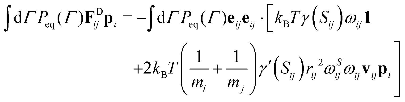
In the standard DPD method, the friction force FDij is defined as
| | 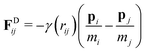 | (1) |
where
pi is the particle momentum,
ri is its position, and
mi, its mass. The coefficient
γ depends only on the interparticle distance
rij = |
ri −
rj| to maintain Galilean invariance, is positive-definite, and is non-zero only if
rij <
rc, where
rc is the cutoff radius. Since the dynamic equation is formulated as a Langevin-like equation for the particle momenta, the latter will vary discontinuously in time due to the action of the random forces, δ
pRij/δ
t in view of
eqn (5). Due to the discrete nature of the algorithm, such variation is finite. Instead, the particle positions are continuous functions although, non-differentiable (
cf.eqn (4)). Therefore, while momenta will change rapidly, positions will vary in a much larger time scale, so that the latter are taken as constants in the integration of momenta in the usual algorithms. This fact is very relevant, as it places the dissipative friction forces within the domain of the so-called linearity between the fluxes and the thermodynamic forces, in Onsager's definition of irreversible phenomena.
14,15 This means that, in the particular case of the standard isothermal DPD, the equilibrium probability distribution for a pair of particles
i and
j is Maxwellian, namely,
Peq ∝ exp[−(
pi2/2
mi +
pj2/2
mj)/
kBT], where
T is the absolute temperature and
kB is Boltzmann's constant. Therefore, for this given pair, we can write the following property,
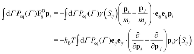
| | 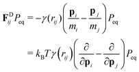 | (2) |
eqn (2) expresses the linearity between the friction force and derivatives of
Peq with respect to the momenta, which ultimately is the corresponding thermodynamic force, according to Onsager. As a consequence, the equilibrium average of the friction force is zero, as
| | 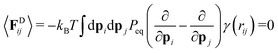 | (3) |
where partial integration has been used to obtain the right-hand side of this last equation. However, if such a linearity is not satisfied because
γ also depends upon the momenta, then one would in general have 〈
FDij〉 ≠ 0, which contradicts the symmetry requirements of the equilibrium state. In the context of the Langevin equations, this is the well-known spurious drift,
16,17 which needs the appropriate correction in the stochastic equation of motion. However, the situation is wider as in some cases no spurious drift is present but nevertheless a corrective term is required, as we will later see. Therefore, along the article we will use the expression spurious behaviour to account for this general situation.
Such linearity is ubiquitous in DPD models, regardless of whether they are isothermal, energy-conserving, or other types. However, in complex fluids, e.g. non-Newtonian liquids, the viscosity depends on the rate of strain. Therefore, since DPD is a coarse-grain model, the simulation of non-Newtonian fluids within the DPD framework should quite naturally entrain friction coefficients depending on the rate of strain, which ultimately depends on the velocity field. From a wider perspective of applications of DPD-like methods (energy-conserving,3,4 GenDPDE,11,18 among others,1,12,13) it is a natural situation to have systems in which the dissipative coefficients, like γ, depend on the fluctuating temperature, the particle relative velocity or any other variable that rapidly fluctuates in a dynamic stochastic equations of motion.
In this article, we address the problem of developing the appropriate dynamic equations for non-linear DPD applications. Although the treatment of the spurious drifts in simple Langevin equations is well known, the required derivation for complex dynamic models like DPD may be daunting if analytically carried out. Together with the derivation of such corrective terms, which is our first important result, in addition we propose a novel numerical method, based on the works of Lax19 and Fixman,20 which allows us to produce the appropriate integration algorithms, consistent with the thermodynamic equilibrium conditions, without the complex analytical derivation of the corrective terms. Moreover, the theoretical analysis permits us to cast the formulation into a clear and generalisable way, which we believe transcends the specific goals of this article.
As a proof of concept, we have applied this framework to reproduce the non-Newtonian behaviour observed in polymeric liquids. Polymers have been simulated using the DPD approach soon after the DPD method was introduced,21–23 including rheological applications in recent times.24,25 All these models have in common that they reproduce the structural complexity of the polymeric molecules with arrays of particles connected by springs, which introduce elastic forces, allow for conformational changes and keep the integrity of the polymer molecule. The non-Newtonian behaviour observed within these types of models arises from the coupling between the externally imposed shear flow and the induced conformational changes of the polymer molecule, which results in a rheological behaviour depending on the rate-of-strain, i.e., the local deformation rate affecting the molecular conformation. In rheological studies,26 the complexity of the mesoscopic model for the polymer can be reduced to a so-called dumbbell model, representing the longest molecular relaxation time, for computational economy. Also rather commonly, the finite extensibility of the chain is included in the FENE dumbbell model.27 Hence, the non-linearity in the rheological response in the dumbbell and general bead-spring models is coupled to the slow dynamics of the internal coordinates of the polymer, namely, the end-to-end distance, associated with the aforementioned longest relaxation time. Therefore, the DPD models used to simulate both the polymer molecule as well as the solvent remain within the framework of the usual linear DPD dynamic models. Therefore, to bring the non-linearity into the DPD model itself, we have introduced a larger degree of coarse-grain in which an, e.g., dumbbell model is virtually embedded in one single DPD particle. Thus, the coupling between the local fluid flow and the polymer conformation is transferred to a specific form of the interparticle friction which depends on the local rate-of-strain, ignoring the dynamics of the internal coordinate. Such an example must reproduce the non-Newtonian behaviour, if the proper selection of the velocity-dependent friction is made. Therefore, the model presented here is the simplest non-linear model within the isothermal DPD framework, and will serve as a proof of the internal consistency of the algorithms introduced in the article. Therefore, the example treated in this article is conceptually relevant and produces the intended non-Newtonian behaviour understandable for the practitioners. However, the importance of our analysis is the generality of the methodology and our ultimate goal is to apply the same scheme to future more complex applications.
The article is organised as follows. In Section 2 we propose the dynamic equations of the standard DPD model, along with the corrections introduced to address the problem of a velocity-dependent friction parameter. We also derive estimators of the local rate of strain, which allows us to formulate a form of the friction parameters depending on these estimators. We also comment on the obtained expressions for the random forces (derived in Appendix A) and introduce the so-called two-step algorithm, which is analysed in comparison with the previous algorithms with corrections. In Section 3 we describe the simulation setup as well as the parameters used in the numerical tests of the algorithm. In Section 4 we analyse and discuss the obtained results. These include, on the one hand, equilibrium simulations to obtain the velocity probability distribution, and the calculation of the zero-shear viscosity using the Einstein–Helfand method. On the other, we study the viscosity of a series of non-equilibrium simulations performed ad increasing stress. Finally, in Section 5 we review the main results obtained in this article.
2 Theoretical framework and analysis
In this section, we start by introducing the isothermal DPD algorithm for a general non-linear model. Next, we define two estimators of the local rate of strain, which are used to produce velocity-dependent friction coefficients, as a case study. Next, we propose the DPD algorithm with the analytical corrections to the spurious behaviour for the cases studied. Finally, we describe the so-called two-step algorithm, which does not require the analytical evaluation of the correction, and prove that it is numerically equivalent to the standard algorithm previously derived.
2.1 The isothermal DPD algorithm
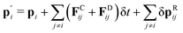
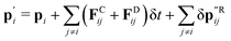
Let us consider that the state of the system at time t is denoted by a point Γ = ({pi}, {ri}) in phase space, where {pi} and {ri} stand for all particle momenta and positions, respectively. The state of the system at t + δt is represented using primed variables as  and is calculated according to the following algorithm:
| |  | (4) |
| |  | (5) |
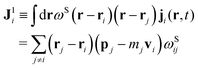
Here, FCij, FDij, and δpRij represent the conservative force, dissipative force, and random momentum exchange between particles i and j, respectively. The expressions for these terms are written as,| | 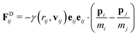 | (7) |
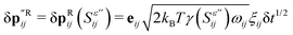
| | δpRij = eij(Γij![[thin space (1/6-em)]](https://www.rsc.org/images/entities/char_2009.gif) ξijδt1/2 + Λijξij2δt + ⋯) ξijδt1/2 + Λijξij2δt + ⋯) | (8) |
In comparison with the standard DPD algorithm, in eqn (7) we have introduced explicitly the dependence of the friction coefficient in the pair relative velocity vij ≡ pi/mi − pj/mj,| | | γij = γ0(rij, vij)ω(rij) | (9) |
which makes the algorithm non-linear, from the perspective of Onsager's theory of irreversible processes.28,29 Notice that the friction coefficient is Galilean invariant, and therefore this new dependence does not impair the overall momentum conservation. Furthermore, angular momentum conservation will require further symmetry properties, which we will discuss when introducing the specific model for the analysis, later on. In the linear model, γ0 is a constant friction coefficient, which here we extend to be a function of the interparticle positions and the relative velocities as well. ω(rij) is a positive definite, monotonously decreasing, spherically symmetric weighting function, which vanishes for rij ≥ rc. In this work, we use the usual quadratic form| |  | (10) |
On the other hand, we have also adopted a more general form of the random contribution, here expressed as a series expansion in terms of ξδt1/2, to indicate that complex forms of the dissipation imply more complex expressions of the random term.16,30 In eqn (8), ξij is a normalized Gaussian number satisfying,| | | 〈ξij(t)ξkl(t′)〉 = 〈δikδjl − δilδjk〉δtt′ | (12) |
where δtt′ is 1 if t and t′ belong to the same time interval in discrete-time simulations, and 0 otherwise.
The random force can then be defined from the random momentum exchanged, according to
| | 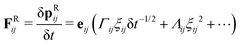 | (13) |
Notice that the random force in a discrete algorithm depends on the size of the time step.
31 In the expressions above,
rij = |
rij|, and
eij =
rij/
rij.
The coefficients Γij and Λij are calculated from the appropriate fluctuation–dissipation theorem later on, as they depend on the specific model used for the non-linear friction coefficient.
2.2 Local estimator of the rate of strain
Before the form for the non-linear friction coefficient is given, in this section we analyze the expected form for the local rate of strain estimator experienced by the central particle i. To this end, in analogy with smoothed particle hydrodynamics,18,32 we review the formulation of the momentum transport equations from a Lagrangian perspective.
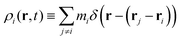
Let us define the momentum density j and mass density ρ according to,
| |  | (14) |
| |  | (15) |
where
r is a field point. Classically, the so-called baricentic velocity field
v is defined from the relation
| | | j(r, t) ≡ ρ(r, t)v(r, t) | (16) |
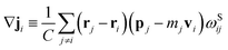
The local rate of strain in a given point of the fluid is thus associated to the components of the velocity gradient tensor ∇
v. In what follows, we estimate the value of such rate of strain from particle coordinates and momenta.
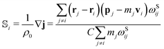
Let us define the local momentum density around a particle i as,
| |  | (17) |
We can now introduce several moments of the momentum density in the immediate vicinity of particle
i. The zero and first-order moments are defined as,
| | 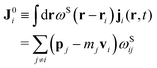 | (18) |
| |  | (19) |
In these equations,
ωSij is a weighting function, positive-definite and with a finite range,
rc. The superscript “
S” indicates that this weighting function is not necessarily equal to that of
eqn (10). Higher-order moments can be defined although they are not relevant for our analysis. Hence, from a continuum standpoint, let us introduce a multipolar expansion of the local momentum density around particle
i| | | ji(r, t) ≈ (r − ri)·∇ji + (r − ri)(r − ri):∇∇ji +⋯ | (20) |
where the zero-order term has been omitted as is zero by construction. Thus, retaining terms only up to the first order, we can write
| |  | (21) |
Due to the isotropy of the kernel together with the homogeneity of the system, this integral is approximately zero, to the lowest order. On the other hand,
| |  | (22) |
The angular integration has been analytically performed due to the isotropy, yielding the identity matrix

and the geometric factor
C, which depends on the mathematical expression for the kernel
ωS. Therefore, comparing
eqn (19) with
eqn (22), we can estimate the local momentum gradient,
i.e.,
| |  | (23) |
We similarly introduce a multipolar expansion of the mass density together with the calculation of the different moments. The local mass density field reads,
| |  | (24) |
In this case, the first non-zero contribution is the zero moment,
i.e.| | 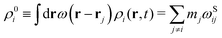 | (25) |
Therefore, we can finally construct the estimator of the rate of strain as a second order tensor,
i.e.,
| |  | (26) |
The expression of  in eqn (26) is multibody, which breaks the pairwise additiveness of the friction forces that is central in the DPD model. Therefore, rather than implementing the estimator as indicated in eqn (26), here we introduce a simplified version involving only pairwise contributions. Although this may seem very restrictive, is sufficient for the purpose of the article that is to show the modifications needed for the standard DPD equations for non-linear situations. Therefore, we choose this simplified model as is sufficient to meet this purpose. Effectively, we decompose
  into pairwise contributions
  , with
| |  | (27) |
We will use this pairwise definition from now on.
2.2.1 Non-linear model for the interparticle friction.
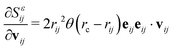
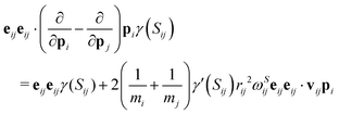
In our simplistic model, we consider a scalar friction γ0cf.eqn (9). We thus use the estimator eqn (27) to introduce a scalar which will modulate the actual friction between two particles, depending on the estimated rate of strain. For the first model, we choose Sαij as| | 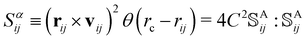 | (28) |
Here, 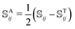 is the antisymmetric tensor, where the superindex T stands for transpose, and we have chosen ωSij = θ(rc − rij). The quantity |rij × vij| is a measure of the rate of the local shearing motion of the particles i and j. However, as constructed, one cannot distinguish between the pure deformation of the local environment of particle i from a pure rigid body rotation of the same environment. To construct such estimator more than two particles are required, as it is expressed by eqn (25). For bounded flows, as in the Couette geometry that we explore in this article, neither free interfaces nor pure rotations are present and the use of such a simplified estimator for the shear rate is pertinent.
For the second model we introduce,
| | 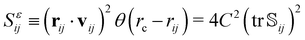 | (29) |
where

stands for the trace of

. For the same reasons expressed before, this estimator cannot distinguish a pure deformation of the volume element from a variation in its volume. The overlapping of these two modes of motion has been recently discussed in the context of other Lagrangian methods like SPH.
18,32
The pairwise additiveness of the local rate of strain proposed in eqn (28) and (29) allows us to discuss the new proposed algorithm for the integration of the non-linear cases.
Next, we propose the velocity-dependent friction coefficient given by,
| | | γij = (γ0e−γ1Sij)ωij ≡ γ(Sij)ωij | (30) |
In this equation,
γ0 is the zero-shear friction coefficient and
γ1 is a prefactor that measures the strength of the shear rate estimator in the form given by either
eqn (28) or (29). The functional form of
eqn (30) is introduced to macroscopically reproduce the shear-thinning behaviour, common in many polymeric materials, as an interesting example to show that the new DPD algorithm is capable of reproducing non-Newtonian behaviour from a non-linear dissipation law.
The two estimators for the local shear given in eqn (28) and (29) require two distinct forms of the fluctuation–dissipation theorem. Effectively, in Appendix A we demonstrate that for the case of eqn (28) it suffices that
| |  | (31) |
We find that, despite the non-linearity of the friction law,
Λij = 0 for this case. However, for the case of
eqn (29) we demonstrate also in Appendix A that,
| |  | (32) |
The presence of the second term (
i.e. Λ ≠ 0) is entirely due to the non-linearity and has to be analytically determined
a priori to construct an explicit algorithm, as in
eqn (4) and (5), with
eqn (6)–(8). Notice that the average of this second term is zero in equilibrium. Therefore, strictly speaking is not a correction of any spurious drift, as also 〈
FDij〉
eq = 0. However, it is a necessary correction needed to produce the Marwell-Boltzmann distribution.
2.3 The two-step algorithm
The analytical calculation of the extra term of the random contribution for the second model can be avoided by introducing an implicit algorithm in two steps. For this analysis, we specialise in the model of eqn (29), which is the only one that requires correction of the spurious behaviour.
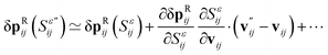
Effectively, let us consider an initial step in which we calculate an intermediate momentum p′′ according to the equation,
| |  | (33) |
with
| |  | (34) |
where the values used for the state variables are evaluated at
t. Next, we reevaluate the friction coefficient using this intermediate momentum,
i.e.,
| |  | (35) |
| |  | (36) |
The corrected random term

is then calculated as,
| |  | (37) |
Then, we finally update the momenta using,
| |  | (38) |
with all the forces calculated at
t and only the random contribution is calculated using the intermediate momenta. It is very important that the random number
ξij used in
eqn (37) is the same sorted to calculate the right-hand side of
eqn (34). We thus state that the use of the corrected random term
eqn (37) in the dynamic equation
eqn (38) satisfies Detailed Balance and, as a consequence, the dynamics of the system correctly samples its equilibrium probability distribution, which is the Maxwellian distribution for the standard isothermal DPD.
To prove the previous statement, we next proceed to demonstrate that the random contribution  is actually identical to the right-hand side of eqn (32), up to the order of validity of the algorithm,
  . We start by expanding eqn (37) up to first order in
  , i.e.,
| |  | (39) |
The first factor in the second term in
eqn (39) can be further developed to obtain,
| | 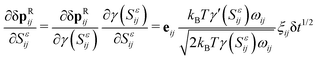 | (40) |
The second factor in turn reads,
| |  | (41) |
Since
eij·
eij = 1, finally, using
eqn (35) to obtain

, substituting
eqn (40) and (41) into
eqn (39) we arrive at,
| |  | (42) |
This expression is identical with
eqn (32), so the two-step algorithm produces the same second-order term in (
ξ2δ
t) as we have determined in Appendix A, as part of the fluctuation–dissipation theorem, provided that the time-step is small enough.
Therefore, the two-step algorithm is an attractive way to deal with non-linear Langevin equations in that the extra term does not require an explicit evaluation. A drawback of the method, however, is that the random number ξij should be used twice: for the estimation of  and for the subsequent calculation of the total random term δpRij.
2.4 Generality and limit of validity of the two-step algorithm
The results obtained in the previous subsection may appear specific to that particular problem, but the applicability of the method transcends this case and can be applied to any problem with the characteristics described here.
Let us consider a mesoscopic system whose state is characterised by a given observable x. In general, we can also consider that along with x its momentum p and internal energy u, complete the description of the state. The equilibrium distribution function in the Canonical ensemble is of the form,
| | 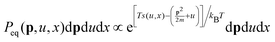 | (43) |
where
s(
u,
x) is the entropy of the system at a given state characterised by (
p,
u,
x), according to Einstein's theory of thermodynamic fluctuations.
33 Denoting,
| |  | (44) |
the so-called thermodynamic force related to the variable
x is
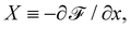
with all the other variables kept constant. In the spirit of Onsager's theory of non-equilibrium thermodynamics, one writes,
which is a definition of the kinetic dissipative coefficient
α. In the linear domain,
α is a constant. However, here we have centered our interest on situations in which
α is a function of the state variable
x. The case of the coupling with other fluctuating variables in the non-linear regime will be addressed elsewhere.
The properties of the random contribution δxR are determined by the Detailed Balance condition, as developed in Appendix A. Proposing a general expansion of the form δxR = Γξδt1/2 + Λ(ξδt1/2)2 + ⋯, as in eqn (8), the evaluation of the first moment yields,
| |  | (46) |
with
Γ = (
p,
u,
x). In general, due to
eqn (44), the following relation is satisfied within the integral,
| | 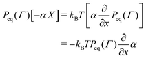 | (47) |
Therefore, ought to 〈δ
xR〉
ξ =
Λ the choice
| |  | (48) |
exactly eliminates this term if ∂
α/∂
x ≠ 0,
i.e., in the non-linear case. Using
(48), the second moment yields
Next, consider the prescription for the two-step algorithm to calculate the first step,
In the second step, the random term then reads,
| | 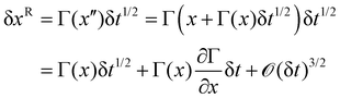 | (51) |
Given the structure of the dynamic equation
eqn (45) and the probability distribution
eqn (43), it is verified that,
| | 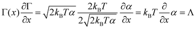 | (52) |
which produces the needed
Λ-term up to

, Q.E.D.
3 Simulation setup
In this section, we detail the setup of numerical experiments designed to investigate the equilibrium and rheological behavior of the system for the different models introduced. Our simulations encompass both equilibrium (EQ) and non-equilibrium (N-EQ) scenarios. For both cases, we utilized the code developed by the Molecular Simulation group at the University of Rovira i Virgili. This code has been validated by several research papers, including Malaspina et al.34 The integration algorithm is a velocity-Verlet and the force loop is parallelised using a nearest-neighbour list.
3.1 Simulation parameters
The simulations are conducted for a system with N = 20000 DPD particles. As we are not using the standard DPD parameters, we have to provide an intuitive picture of the scales used to make the equations dimensionless. We shall assume that there is an underlying physical fluid in a given equilibrium state characterised by a reference pressure and temperature (PR, TR), which we coarse-grain (CG) into a DPD particle via decimation through a scale factor ϕ. The physical number density of the reference state cR and the degree of CG allows us to define a scale of length l = (ϕ/cR)1/3, which is the average distance between DPD particles. The particle mass is m0 = ϕMw/NA, where Mw is the molecular mass and NA is Avogadro's number. For the energy, we take u = PRϕ/cR, rather than kBT, as is the customary choice. The time scale is then  . Using these scales from our reference system, we choose the mass of the DPD particle to be m = 1. We will analyse two different densities, namely n = 16 and n = 32. The dimensionless volume of the system corresponding to n = 16 is V = 1250, while for density n = 32, we selected V = 625. For equilibrium simulations, the box is cubic, with lateral sizes L = 10.77 and L = 8.55 for n = 16 and n = 32, respectively. For N-EQ simulations, the size on the x-direction is Lx = 2L while Ly = Lz = L. Therefore, V = 2L3, which gives L = 8.55 and L = 6.79 for the two densities. Moreover, the dimensionless temperature of our simulated system is 0.1, corresponding to a physical temperature T = 0.1u/kB, should we set the physical value of u. This temperature is used in the random force of the algorithm in all equilibrium and non-equilibrium simulations in this article. The chosen set of parameters does not necessarily correspond to any physical state of the reference system. The selection of the appropriate time-step δt = 10−4 is carefully considered and validated in Appendix B, using the measure of the viscosity to set the appropriate value. Periodic boundary conditions are applied in all three spatial coordinates. The thermalisation induced by the random force physically represents the coupling of the system with a heat reservoir at the same nominal temperature T. However, in the non-equilibrium simulations (cf. Section 3.3), we inject energy into the system, due to the momentum push at each slab, which eventually drains into the reservoir through the dissipative forces. Due to this phenomenon, kinetic temperatures that differ from the nominal temperature of the random force are observed at high rates of strain.
Table 1 provides a summary of the input parameters in dimensionless units. Each simulation variant is assigned a unique identifier for ease of reference: ref represents the reference case with a γ1 = 0 (see eqn (30)), corresponding to the standard isothermal DPD. Cross and Dot cases feature the two estimators used in the simulations, according to eqn (28) and (29), respectively, while the Two-step-dot case corresponds to the parameters used in the application of the two-step algorithm with the Dot estimator.
Table 1 Simulation parameters. We have labelled each simulation according to the rate of strain estimator or reference model. To address the different densities along the article we use digits next to the label. For example Dot32 indicates density 32 for case Dot
| Particles (N) |
γ
0
|
γ
1
|
k
B
T
|
r
c
|
δt |
Label |
| 20000 |
5 |
0 |
0.1 |
1 |
10−4 |
Ref
|
| 20000 |
5 |
1 |
0.1 |
1 |
10−4 |
Cross
|
| 20000 |
5 |
1 |
0.1 |
1 |
10−4 |
Dot
|
| 20000 |
5 |
1 |
0.1 |
1 |
10−4 |
Two-step-dot
|
For simplicity, we choose to set the conservative forces (FCij = 0) across all models. This type of DPD model is often referred to as ideal DPD.
3.2 Equilibrium probability distribution simulations
The test on the thermodynamic consistency of the algorithm requires the evaluation of the equilibrium probability distribution of the particle momenta. Methodologically, once the system is equilibrated, we record the modulus of the velocity of all the particles for the last 2000 time-steps (over 40 million samples), and classified them in 150 bins, for velocities ranging from 0 to 2 in dimensionless units. The resulting histogram is normalised and then compared to the theoretical Maxwell–Boltzmann velocity distribution, for the same nominal temperature and particle mass, i.e.,| | 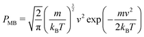 | (53) |
where| |  | (54) |
The parameters of the simulations are the same as in Table 1.
3.3 Non-equilibrium viscosity calculations
For the non-equilibrium simulations, we employ a variation of the boundary-driven PeX algorithm, a method originally introduced by Müller-Plathe et al.35,36 The PeX method used for viscosity calculations31 considers a simulation box with Lz = Ly = L and Lx = 2L with two narrow slabs defined at specific positions along the x-axis, dividing the simulation box into two identical moieties, across the periodic boundary conditions. The centre of the box is considered as the coordinate origin, and the slab centres are located at x1 = −Lx/4 and x2 = +Lx/4, each with a width of Δx = Lx/10 (see Fig. 1). In the original method,36 a virtual elastic collision was produced between the particle with larger −vz in slab at x1 and that of larger vz in the slab at x2. Such collision transfers a net amount of momentum between the slabs Δpz, which eventually produces a net flow within the slabs in the directions given in Fig. 1, while conserving total momentum and energy. If this process is repeated every Δt, the system eventually arrives to a steady state, where a linear velocity gradient develops in each of the two moieties in which the system is divided. The stress Πzx exerted onto every slab can be obtained from the ratio,| |  | (55) |
where ΣΔpz stands for the accumulated momentum transferred over a given period of time Δt, after the steady state is reached. Notice the factor 2 in the denominator due to the propagation of the stress to the two halves of the simulation box. At the same time, phenomenologically one has,| |  | (56) |
which is the constitutive equation that relates the exerted stress with the velocity gradient through the viscosity of the system, μ. Therefore, once the velocity gradient dvz/dx is measured, as the stress is known and constant across the simulation box, its ratio is the measure of the viscosity. However, if the original procedure is to be used, the maximum velocity gradient that can be obtained is limited by the width of the velocity distribution function. Effectively, such width is of the order of 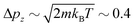 (the latter, in dimensionless units). For the problem that we are addressing, this difference is not enough to produce high shear rates. We have thus introduced a variation in the original PeX method replacing the virtual collision by simply adding +Δpz to the selected particle with minor vz in slab 1 and −Δpz to that with major vz in slab 2 every δt, with no restriction on the size of Δpz. Although the total momentum conservation is maintained, the energy is not, as the procedure effectively pumps kinetic energy into the system. In the steady state, such energy influx is eventually dissipated by the friction forces, but the kinetic temperature of the system is therefore affected by the viscous heating. For each model and density, we have considered several cases characterised by a momentum Δpz transferred at every time-step, as indicated in Tables from 3 to 7. The resulting velocity profile, vz(x), is determined by dividing the whole box in the x-direction into 40 bins. At given instants of time, a snapshot of the system is taken and the z-component of the velocity field is obtained from the following average over the bin,
| | 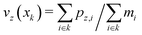 | (57) |
where k here indexes the bin. The procedure is repeated at different decorrelated instants. The final velocity profile is ultimately obtained from an average over a number of 5000 instantaneous profiles. Next, we calculate the resulting velocity gradient over a sufficiently wide region in the middle of the box, where the profile is linear, by a linear regression.
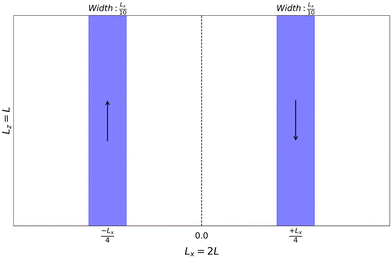 |
| | Fig. 1 Visualizing the slabs' configuration and added momentum direction in our N-EQ simulation. | |
The dynamic temperature Td field is determined from the kinetic energy in the directions orthogonal to the streaming motion, according to the energy equipartition relation,
| |  | (58) |
where
Nk is the number of particles in the
kth bin. Notice that in equilibrium
Td =
T enforced by the fluctuation–dissipation theorem, according to either
eqn (31) or (32).
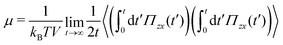
3.4 Validation with Einstein–Helfand zero-shear viscosity calculations
For verification purposes, we have conducted equilibrium simulations to determine the zero-shear viscosity of the Cross and Dot non-linear models, along with the two-step algorithm, using the Einstein–Helfand (EH) method, to validate the non-equilibrium simulations at vanishing rate of strain. The test also serves to validate that the dynamics induced by the two-step algorithm are consistent with the standard algorithms for non-linear models.
To obtain the numerical values of the viscosity in equilibrium, we employ the method developed by Malaspina et al.31 In this reference, the authors propose the use of the standard Einstein–Helfand formula,37
| |  | (59) |
where
V denotes the volume, whereas the relevant
xz-component of the stress tensor
Πzx is given by the expression,
| | 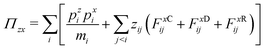 | (60) |
as demonstrated in ref.
31. In our analysis, we have considered an ideal DPD model,
i.e.,
FCij = 0. Moreover, notice that the random force is defined from
eqn (13) and therefore also contains second-order terms,

used to correct the spurious contributions due to the non-linear friction. This fact is in agreement with the mechanistic interpretation of the stress tensor given in ref.
31. For the two-step algorithm, the contribution of
FRij to the stress is calculated using the value of the random force after the first step.
Finally, to avoid finite-size effects in the evaluation of the correlation function, we must consider the linear portion up to a limiting time, tmax ≪ L2/4π2ν, where L is the size of the simulation box and ν = μ/ρ is the evaluated kinematic viscosity of the model (see ref. 31 for details).
4 Results and discussion
In this section, we present the outcomes of the numerical simulations proposed earlier. First, the equilibrium (EQ) simulations, on the one hand, are used to test the capacity of the non-linear models to correctly sample the equilibrium distribution. On the other, the zero-shear viscosity obtained from the EH correlation is used to also test the dynamics of the models, as that viscosity should be consistent with the non-equilibrium measurements at vanishing shear, as well as with the properties of the standard linear model.
Second, the non-equilibrium (N-EQ) simulations are performed at the increasingly larger rate of strain (shear rate), where the features of the non-linear model are revealed at large shear rates. To correctly interpret the measured viscosity we have to consider that two contributions to the viscosity exist in ideal DPD models.38 The kinetic contribution is due to the momentum transport due to particle agitation. This contribution scales as kBTd/γrc3, and is independent of the particle density. It is thus expected that this contribution will increase with decreasing friction and increasing dynamic temperature Td. Both situations will simultaneously occur at high shear rates. The second contribution is purely dissipative and is in turn proportional to γn2rc5. Therefore, to observe the shear thinning behaviour39 we have selected simulation parameters such that, at least in equilibrium, the model's viscosity is dominated by the dissipative contribution, which will decrease with decreasing interparticle friction. The condition of dominating dissipative contribution is satisfied always that kBTd ≪ γ2n2rc8 for the ideal DPD case,8 analised along this article.
4.1 Maxwell–Boltzmann distribution
The thermodynamic consistency of the algorithms proposed requires that the dynamics of the resolved variables sample the appropriate equilibrium distribution, set by the principles of statistical mechanics. For the present case of an ideal DPD model, the resolved variables are particle positions and momenta. Therefore, in equilibrium, with no external fields acting on the particles, the relevant distribution should be Maxwell–Boltzmann for particle momenta.
In Fig. 2, we present the validation tests regarding Cross16, Dot16 and Two-step-dot16 models as described in Table 1. All the simulations produce the appropriate distribution at the nominal temperature T set by the random forces, according to eqn (31) or (32). As it is clear from the figure, all the plots are indiscernible from the theoretical curve (dashed line), showing that all the algorithms generate dynamics that evolve to the appropriate thermal equilibrium. In particular, notice that the two-step algorithm gives an excellent agreement with the theoretical distribution. Therefore, its thermodynamic consistency is verified. This is the first important result of the present article.
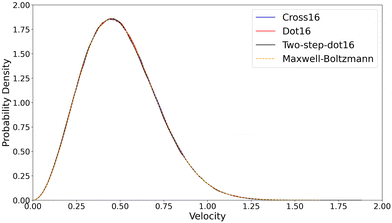 |
| | Fig. 2 Velocity distribution function computed in EQ simulations compared to the Maxwell–Boltzmann distribution at the same temperature. We tested the Cross16, Dot16 and Two-step-dot16 models with T = 0.1. The rest of the parameters are given in Table 1. | |
4.2 Analysis of the zero-shear viscosity
We have selected a minimal momentum transfer of Δpz = 0.01 to produce the smallest stress in all models (see Table 3), which allows us to work within the linear response regime in the calculation of the viscosity through the induced velocity gradient, according to eqn (55). In this regime, the friction experienced by the particles is the value of the equilibrium friction.
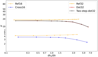
Fig. 3 shows the obtained velocity profile, in which an extended linear region in each of the two moieties is observed. The velocity gradient is thus obtained from this linear part. These two linear regions are connected through a smooth transition across the slab, as expected. Table 2 collects the results of the zero-shear viscosity obtained from the N-EQ simulations, compared to EH results from EQ simulations. The N-EQ results and the EH values are in a very good agreement in all cases. Here, we have to stress that the results obtained from cases Dot and Two-step-dot are also in perfect agreement with each other for both, the EH calculation of the shear viscosity and the low-shear limit of the N-EQ simulations, as well. Therefore, the two-step algorithm also produces dynamic consistency, which constitutes the second important result of this article.
 |
| | Fig. 3 Averaged velocity profile and corresponding linear regression in the middle area for the N-EQ Cross16 case with Δpz = 0.01. The regions where the velocity gradient changes sign correspond to the position of the slabs. | |
Table 2 Zero-shear viscosity results for EH and N-EQ methods. Numbers inside the parentheses next to names indicate the density, while the digit inside the parentheses in the ciphers represent the error in the estimation
| Case |
EH (16) |
N-EQ (16) |
EH (32) |
N-EQ (32) |
|
Ref
|
4.223(4) |
4.29(3) |
18.443(4) |
18.2(2) |
|
Cross
|
3.985(1) |
3.72(3) |
15.87(1) |
15.87(6) |
|
Dot
|
4.082(2) |
3.99(2) |
17.171(5) |
16.81(9) |
|
Two-step-dot
|
4.193(2) |
3.95(2) |
16.78(1) |
16.83(9) |
4.3 Non-linear regime: shear-thinning
Shear thinning, also known as pseudoplasticity, is a property of certain fluids where the viscosity decreases as the rate of strain increases. This behavior contrasts with the response of Newtonian fluids, for which the viscosity remains constant, independently of the shear rate (see ref. 39 for details). With our choice of parameters, selected to make the dissipative contribution much larger than the kinetic, it is expected that a significant decrease of the friction coefficient between the particles would produce a decrease in the viscosity, showing the aforementioned shear-thinning behaviour. In Tables 3 and 4 we show the results for the viscosity as a function of the rate of strain of the Ref16 linear and the Cross16 non-linear cases, respectively. The two sets of simulations are performed at the same overall density, nominal temperature T, and stress. The tables also gather the values of the stress, the velocity gradient and density in the central region, for completeness. For the reference case Ref16, we observe that the density in the central part of the simulation box and kinetic temperatures are close to the nominal ones over the whole range of stresses analysed. A slight increase of the kinetic temperature with the stress, accompanied by a slight increase in the shear viscosity, linearly proportional to the kinetic temperature, is observed. Therefore, the slight non-Newtonian behaviour of the case Ref16 is due to the increase of the kinetic contribution as a result of the heating of the system as the energy introduced through the stress is increased. As far as the Cross16 case is concerned, Table 4 shows a clear decrease of the viscosity with the shear rate. This is the signature of the shear-thinning behaviour induced by the non-linear friction. For this case, the increase of the temperature is, however, more noticeable than for the Ref16 case. Such an increase of the temperature is related to the viscous-heating proportional to Πzx∂vz/∂x. As the stress is the control parameter, the smaller the viscosity, the larger the shear rate and, therefore, the larger the dynamic temperature. As a consequence, increasing the stress imposed on the system eventually makes kBTd > γ2n2rc8 and the kinetic viscosity dominates the overall behaviour (not shown). Therefore, the shear-thinning is only observed in a window of externally imposed stresses satisfying simultaneously the two conditions, γ1Sij ≥ 1 (cf.eqn (30)) and kBTd ≪ γ2n2rc8.
Table 3 Results of N-EQ simulations for the Ref16 case (cf.Table 1). All quantities are evaluated at the central linear region between the slabs
| Δpz |
Π
zx
|
dvz/dx |
T
d
|
Density |
μ
|
| 0.01 |
0.68 |
0.160(1) |
0.1002(1) |
16.0(1) |
4.29(3) |
| 0.025 |
1.71 |
0.397(5) |
0.1011(1) |
16.0(1) |
4.31(5) |
| 0.05 |
3.42 |
0.784(4) |
0.1033(1) |
16.0(1) |
4.36(2) |
| 0.075 |
5.13 |
1.153(9) |
0.1061(1) |
15.89(7) |
4.45(3) |
| 0.1 |
6.84 |
1.522(6) |
0.1089(1) |
15.92(9) |
4.49(2) |
| 0.15 |
10.26 |
2.247(1) |
0.1141(2) |
15.87(3) |
4.57(2) |
| 0.2 |
13.68 |
2.92(2) |
0.1192(3) |
16.01(7) |
4.69(4) |
Table 4 Results of N-EQ simulations the Cross16 case
| Δpz |
Π
zx
|
dvz/dx |
T
d
|
Density |
μ
|
| 0.01 |
0.68 |
0.184(2) |
0.1001(1) |
16.0(1) |
3.72(3) |
| 0.025 |
1.71 |
0.460(5) |
0.1006(2) |
16.0(1) |
3.72(4) |
| 0.05 |
3.42 |
0.936(7) |
0.1031(1) |
16.1(1) |
3.65(3) |
| 0.075 |
5.13 |
1.425(9) |
0.1057(1) |
16.20(7) |
3.60(2) |
| 0.1 |
6.84 |
1.99(1) |
0.1089(1) |
16.39(5) |
3.44(2) |
| 0.15 |
10.26 |
3.54(2) |
0.1199(6) |
16.75(9) |
2.89(2) |
| 0.2 |
13.68 |
5.91(6) |
0.146(2) |
17.05(8) |
2.31(3) |
When using the Dot estimator, the window of shear rates where the shear-thinning behaviour is observable is reduced when using n = 16. To increase the weight of the dissipative contribution to the viscosity, we performed N-EQ simulations at higher density n = 32. The behaviour of this estimator is particularly important as its use requires correction of the spurious drifts due to the non-linear friction, unlike the Cross estimator. In addition, the former is the benchmark for the analysis of the performance of the two-step algorithm. In Tables 5–7 we present the values of the viscosity as a function of the shear rate, along with the dynamic temperature and the density in the linear region in the centre of the simulation box. We observe that the viscosities of the Dot32 and Two-step-dot32 are practically the same, as they are also the measured dynamic temperature, density and shear rate. We can thus conclude that the two algorithms are producing the same dynamics and that their results are indiscernible from each other. This is the third important result: in DPD simulations with non-linear models for friction, the use of the two-step algorithm permits a consistent dynamic simulation without the explicit calculation of the correction to the spurious drift. As they are structurally identical, the presence of a temperature-dependent thermal conductivity in DPDE and GenDPDE models can be also tackled using a two-step algorithm. The problem of temperature-dependent friction in DPDE and GenDPDE will be addressed elsewhere.
Table 5 Results of N-EQ simulations for Ref32 case
| Δpz |
Π
zx
|
dvz/dx |
T
d
|
Density |
μ
|
| 0.025 |
2.71 |
0.149(1) |
0.1001(1) |
32.0(4) |
18.2(2) |
| 0.075 |
8.14 |
0.444(3) |
0.1010(2) |
31.8(4) |
18.4(1) |
| 0.15 |
16.29 |
0.882(4) |
0.1018(4) |
31.8(3) |
18.47(9) |
| 0.2 |
21.72 |
1.172(2) |
0.1048(2) |
31.7(2) |
18.52(3) |
| 0.25 |
27.14 |
1.45(1) |
0.1065(3) |
31.6(4) |
18.7(1) |
| 0.3 |
32.57 |
1.740(7) |
0.1079(1) |
31.8(3) |
18.72(8) |
| 0.4 |
43.43 |
2.300(9) |
0.1112(3) |
31.5(3) |
18.89(8) |
| 0.5 |
54.29 |
2.84(1) |
0.1142(3) |
31.8(3) |
19.1(1) |
| 0.55 |
59.72 |
3.11(2) |
0.1156(4) |
32.0(3) |
19.2(1) |
Table 6 Results of N-EQ simulations for Dot32 case
| Δpz |
Π
zx
|
dvz/dx |
T
d
|
Density |
μ
|
| 0.025 |
2.71 |
0.162(1) |
0.1002(1) |
31.9(4) |
16.81(9) |
| 0.075 |
8.14 |
0.485(4) |
0.1015(2) |
31.8(4) |
16.8(1) |
| 0.15 |
16.29 |
0.981(4) |
0.1050(4) |
31.9(3) |
16.60(6) |
| 0.2 |
21.72 |
1.31(1) |
0.1085(6) |
31.8(4) |
16.5(2) |
| 0.25 |
27.14 |
1.678(9) |
0.1128(8) |
32.1(4) |
16.18(8) |
| 0.3 |
32.57 |
2.070(7) |
0.118(1) |
32.1(2) |
15.73(5) |
| 0.4 |
43.43 |
2.90(2) |
0.1350(9) |
32.7(4) |
15.00(6) |
| 0.5 |
54.29 |
4.53(7) |
0.20(1) |
31.6(7) |
12.0(2) |
| 0.55 |
59.72 |
6.3(3) |
0.22(1) |
33.3(3) |
9.5(4) |
Table 7 Results of N-EQ simulations for Two-step-dot32 case
| Δpz |
Π
zx
|
dvz/dx |
T
d
|
Density |
μ
|
| 0.025 |
2.71 |
0.161(1) |
0.1001(2) |
32.0(3) |
16.83(9) |
| 0.075 |
8.14 |
0.481(2) |
0.1014(2) |
32.2(5) |
16.94(9) |
| 0.15 |
16.29 |
0.986(8) |
0.1054(2) |
31.8(4) |
16.5(1) |
| 0.2 |
21.72 |
1.316(8) |
0.1086(3) |
32.1(4) |
16.5(1) |
| 0.25 |
27.14 |
1.680(9) |
0.1134(3) |
32.0(3) |
16.15(9) |
| 0.3 |
32.57 |
2.06(2) |
0.1186(7) |
32.2(4) |
15.8(2) |
| 0.4 |
43.43 |
2.86(1) |
0.134(1) |
33.1(2) |
15.19(2) |
| 0.5 |
54.29 |
4.5(4) |
0.200(5) |
31.7(5) |
12.2(3) |
| 0.55 |
59.72 |
6.2(2) |
0.21(1) |
28.6(8) |
9.6(3) |
In Fig. 4 we summarise the behaviour of the viscosity vs. the rate of strain for the cases analysed. First, we observe a region in which the behaviour of the non-linear cases and the linear reference case are analogous. Notice that in this region the measured viscosity is practically identical to the zero-shear viscosity of Table 2 for each individual case. However, the viscosities of the non-linear models are slightly inferior to the reference cases due to thermal agitation that makes 〈e−γ1Sij〉 ≤ 1. Second, after a given critical rate of strain  , the non-linear models show a decreasing viscosity, while the reference cases do not. The slight increase of the viscosity in the reference linear case is also observed in Ref32. In Fig. 5 we have plotted the variation of the dynamic temperature as a function of the viscous heating. The plot shows a rather linear dependence of the temperature with the dissipation rate calculated at the centre of the box. We have included the cases Dot16 and the Two-step-dot16 to show that the increase of the temperature is the steepest. Due to this effect, there is no range within which a shear-thinning behaviour can be observed. In general, from Fig. 5 we can conclude that for the DPD models analysed the dynamic temperature varies inversely proportional to the actual value of the friction between the particles. Apart from the characteristic shear-thinning behaviour observable in the N-EQ simulations for both the Dot and Cross cases, we highlight that the two-step algorithm produces the same results for all properties measured in the simulations as found with the use of the standard algorithm with the random force eqn (32). Therefore, the corresponding plots in Fig. 4 closely follow each other.
 |
| | Fig. 4 The viscosity as a function of the shear rate in N-EQ simulations shows the effect of non-linear friction implemented via the local strain rate estimators, Cross and Dot. | |
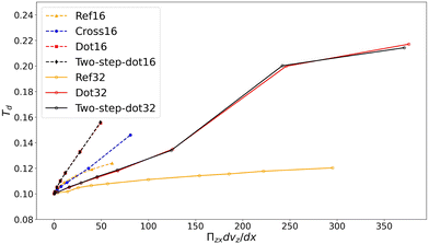 |
| | Fig. 5 Averaged temperature (eqn (58)) vs. entropy production in N-EQ simulations. | |
4.4 Inhomogeneities in the non-linear regime
The dependence of the viscosity on the rate of strain induces local inhomogeneities around the slabs, where the energy and momentum injection take place. Although this analysis is not the main objective of the present article, we discuss this problem for completeness.
We have investigated the temperature profile across the system, using the same method as in Section 3.3, dividing the box in the x-direction into 40 bins and using eqn (58) to obtain the dynamic temperature in each bin. Similarly, employing a time-averaging method, we determined the density profile for all cases by counting the number of particles in each bin. This procedure provides the dependence of the fields in the x-direction, assuming translational invariance in the z-direction. However, to understand the figures we have to take into account that the PeX procedure introduces momentum every time-step in a localised position along the z axis. Due to the interaction between the affected particle and its immediate vicinity, this effect is equivalent to the introduction of Πzz stress of the order of  which creates local inhomogeneities in the velocity vz along the z-axis, namely δvz. We can consider that, at high shear rates, the motion of the kicked particle inside the slabs scatters the neighbouring particles, inducing a δvx component in localised places along the z-axis. In steady state, this effect is balanced by a gradient in pressure from the outer regions, to reach the mechanical equilibrium in the x direction. As this effect is mechanical, it is not reflected in the dynamic temperature of the slab. Hence, no local equilibrium can be properly defined. This consideration is very important to understand the nature of the inhomogeneities found during the simulations.
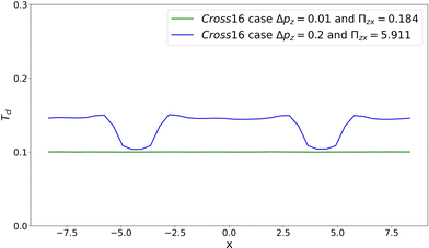
In Fig. 6, we show the dynamic temperature profile across the system for the Cross16 at low and large shear rates. In the larger shear rate employed, we observe that the slabs are colder than the central part of the system. This is due to the fact that there is no viscous heating inside the slabs, as the velocity profile is almost homogenous (see Fig. 8), leaving the temperature of the slab approximately equal to the nominal temperature of the random force. The injected energy does not increase the thermal agitation within the injection region. However, the temperature in the central part of the system is higher than the nominal. The energy introduced in the slab is uniformly dissipated in the central part, causing a temperature rise due to viscous heating.
 |
| | Fig. 6 Comparison of averaged temperature profiles (Td) for N-EQ Cross16 scenarios: low-shear (Δpz = 0.01) vs. high-shear (Δpz = 0.2) cases. | |
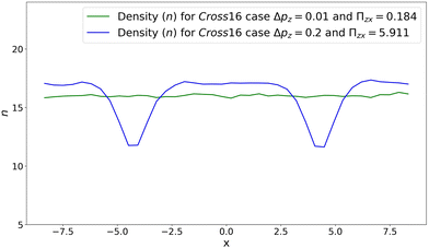
In Fig. 7, we compare the average density profiles for the same situations as in the previous case. Here, we observe a depletion of the slabs and an increase of the concentration in the central region of the two moieties of the simulation box. As the modelled system is thermodynamically equivalent to an ideal gas, i.e., P = nkBT, Fig. 6 and 7 contradict local equilibrium, as the pressure in the centre of the box would be higher than the pressure within the slab if we apply the previous equation of state with the local dynamic temperature at each region. However, if we consider the energy pumped inside the slab to estimate am effective temperature Teff = Td + Δpz2/2mkB, we obtain that the pressure values are very similar.
 |
| | Fig. 7 Comparison of averaged density profiles for N-EQ Cross16 scenarios: low-shear (Δpz = 0.01) vs. high-shear (Δpz = 0.2) cases. | |
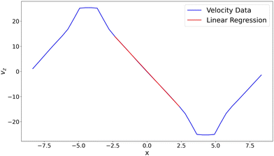
Finally, we analyse the velocity profile at high shear rate in Fig. 8, for the same Cross16 system at high shear rate. Compared to Fig. 3, the velocity profile at high shear rate, shows indications that the slabs are somehow detached from the rest of the system. Effectively, the regions of large shear rate are concentrated at the contact area between the slabs and the bulk of the system. As the stress Πxz is constant outside the slabs for the present Couette flow, the product viscosity times velocity gradient is constant across the system. Therefore, these regions of large shear are also the regions with the lower viscosity, which is responsible for such a detached motion of the slabs. This behaviour is similar to that observed in polymeric flows in ducts, where at high Deborah numbers a region of strong velocity change develops near the walls.39
 |
| | Fig. 8 Velocity profile and corresponding linear regression in middle area for the N-EQ Cross16 case with Δpz = 0.2. | |
To end this section, let us mention that even in the large shear rate situations, the measure of the viscosity is possible even under the presence of such inhomogeneities caused by the strong shear and the non-linear behaviour. The constant stress, together with the linear profile in the centre of the box allows us to obtain a significant value for the non-linear viscosity, using eqn (56).
5 Conclusions
The analysis presented in this article highlights the efficacy of the proposed model in accurately simulating complex fluids, in which the transport coefficients depend on the fast-fluctuating variable, the particle velocity in our analysis. We have derived the appropriate form of the random force, by proposing an expansion in powers of ξδt1/2, and determining the two leading coefficients through the application of Detailed Balance to the dynamic transitions. Moreover, we have further demonstrated that our two-step algorithm naturally produces the sought correction for the non-linear friction behaviour, which is our main result presented in this article. The analysis performed with both, the expanded random force and the two-step algorithm, shows that the model not only captures the intricate behavior of complex fluids, like non-Newtonian polymer liquids, but also compensates for any spurious drifts induced by the stochastic equation of motion for the DPD model. This fact suggests that our approach holds significant promise for a wide range of applications requiring precise modelling of complex fluid dynamics. The extension of the analysis to models with more than one fast random variable, like in the recently developed GenDPDE and GenDPDE-M, must provide an enhancement of the capabilities of these simulation techniques to model complex systems at the mesoscale.
Author contributions
A. N., C. S. and J. B. A. have contributed to the investigation, methodology, formal analysis, validation, visualisation and writing of the original draft. In addition, JBA has contributed to the conceptualisation and project management.
Data availability
The relevant data is included in the body of the article. Row data from simulations can be provided by the authors upon request.
Conflicts of interest
There are no conflicts to declare.
Appendices
A Derivation of the statistical properties of the random terms from detailed balance
Within this appendix, we derive the statistical properties of the random contribution from Detailed Balance, which is based on the time-reversibility of the microscopic trajectories of the underlying physical system.16 Schematically, as mentioned earlier, the algorithm provides a transition from a state point Γ = ({pi(t)}, {ri(t)}) at time t to a new point Γ′ at time t + δt. The new point is a function of the original one, the dynamic properties of the system, and of the random number ξ. The overall algorithm can be written in the following general form:where Γd represents the generic function that provides the dynamics, and its arguments represent the variables on which this function depends. The transition probability is thus given by| | | w(Γ → Γ′)δt = 〈δ(Γ' − Γd[Γ, ξ; δt])〉ξ | (62) |
The subscript ξ indicates that the average has to be determined over all realizations of the random number ξ. From this expression it follows that| |  | (63) |
The reverse trajectory is defined as Γ* → Γ*′, where 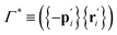 and Γ*′ ≡ ({−pi}, {ri}). The change of sign depends on the parity under time reversal of the variable.16 Thus, detailed balance indicates that
| | | Peq(Γ)w(Γ → Γ') = Peq(Γ*)w(Γ* → Γ*′) | (64) |
This last equation permits us to calculate the moments of the distribution. If we restrain the analysis up to second-order moments,16 we are under the same degree of approximation as the Fokker–Planck equation.
A.1 First moment
To obtain the first moment of the momentum distribution, let us consider the equality| | 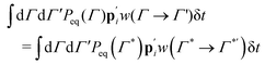 | (65) |
Notice that, on the right-hand side of this equation we can write  . Hence, the integration over Γ*′ can be readily performed. Using (63) we can write,
| | 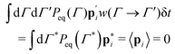 | (66) |
where we have also introduced the change of the integration variable. From this equation, using (5) and after simplifications, we have| | 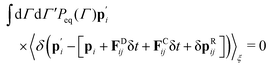 | (67) |
Integrating over Γ′ one finds,| | 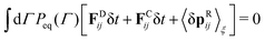 | (68) |
First, notice that, by construction, 〈FCij〉 = 0. Second, the average over the random number only affects the random term. Third, we have to analyse the average of the dissipative force in more detail, i.e.,| |  | (69) |
Using partial integration and that the probability distribution exponentially decays at the limits of the variable domain, we can further write,| | 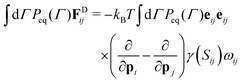 | (70) |
The right-hand side of this last equation can be further developed to give,| |  | (71) |
Next, we explicitly evaluate the gradient of the estimator using eqn (28), which gives,| | 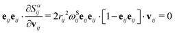 | (72) |
Thus, for this estimator, eqn (71) identically vanishes. In the case of the second estimator, eqn (29), one has| | 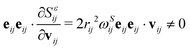 | (73) |
For this second case, we thus have,| |  | (74) |
However, the fact that the result is linear in the momentum, means that the average of this term is also zero. Therefore, the equilibrium average of the dissipative force is zero and there is no spurious drift. Therefore, to satisfy eqn (67) the equilibrium average of the second term should yield,In view of eqn (8), the average of δpRij over the random number ξ gives,| | | 〈δpRij〉ξ = Λijδt | (76) |
For convenience, as it will be apparent below, we can choose,| | 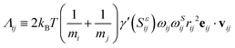 | (77) |
Obviously, the equilibrium average of this contribution vanishes.
A.2 Second moment
The starting point of the calculation is| | 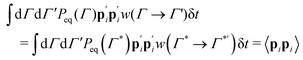 | (78) |
where, in deriving the last equation, we have used the same arguments as for the first moment. Using again eqn (5), we can write,| | 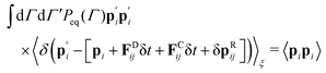 | (79) |
Again, integrating over Γ′ and keeping terms up to first order in δt only, we can write,| | 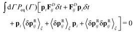 | (80) |
The contributions of the form 〈piFCij〉 do not appear because are zero as they are odd functions of the momentum. In turn, the contributions of the form and pi〈δpRij〉ξ are non-zero because of the quadratic term proportional to ξij2δt. We have also cancelled the term 〈pipi〉 as it appears on both sides of the equation. Hence, keeping terms up to first order in the time-step, one has,| |  | (81) |
Next, let us analyse the term 〈FDijpi〉. Using the explicit form of the dissipative force, we can write,
| |  | (82) |
The differentiation in the integrand produces the classical result, plus a correction due to the non-linearity of the friction coefficient, namely,
| |  | (83) |
where only
eqn (74) has been considered, as for model
Cross this contribution vanishes, in view of
eqn (72). Since
, we can thus write
| |  | (84) |
The transposed matrix follows similarly. Next, notice that, in view of the definition in
eqn (77), the second term on the right-hand side of
eqn (84) is identically cancelled. The same occurs with the transposed. We are thus left with the equality,
| |  | (85) |
where the factor 2 comes from the transposed. Therefore, for
j≠
i we can choose
In this way, the fluctuation–dissipation theorem is completely defined.
B Convergence test
To select the appropriate time-step (δt), we examined the effect of the latter on the measured viscosity in the N-EQ simulations. We conducted simulations for both the Dot16 and the Two-step-dot16 cases, focusing on the largest stress applied, namely 13.68. As the time-step is changed, the transferred momentum has to be adjusted to obtain the same imposed stress, in view of eqn (55). In Table 8 we summarize the obtained results. Since the errors related to the viscosity calculations are negligible in this scale, we opted to not add them to this table.
Table 8 Effect of δt on μ in Dot16 (DT) and Two-step-dot16 (TS) cases
| δt |
Δpz |
Π
zx
|
dvz/dx-DT |
dvz/dx-TS |
μ-DT
|
μ-TS
|
| 0.05 |
100.00 |
13.68 |
0.2449 |
0.2447 |
55.86 |
55.90 |
| 0.01 |
20.00 |
13.68 |
2.1302 |
2.1335 |
6.42 |
6.41 |
| 0.005 |
10.00 |
13.68 |
4.3291 |
4.3149 |
3.16 |
3.17 |
| 0.001 |
2.00 |
13.68 |
3.5729 |
3.5727 |
3.83 |
3.83 |
| 0.0005 |
1.00 |
13.68 |
3.5714 |
3.5498 |
3.83 |
3.85 |
| 0.0001 |
0.20 |
13.68 |
3.5973 |
3.5865 |
3.80 |
3.81 |
Fig. 9 presents the viscosity values plotted on a logarithmic scale against the logarithm of δt, the latter in reverse scale. Notably, viscosities for δt smaller than 0.001 converge to a specific value in both cases, indicating that our choice of δt = 10−4 falls within the acceptable range.
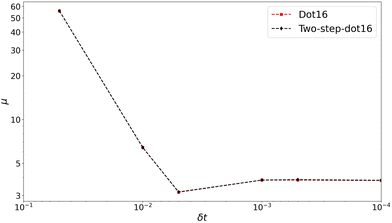 |
| | Fig. 9 Effect of decreasing δt on the viscosity, for Dot16 and Two-step-dot16 cases. Note the values in the x-axis are decreasing. | |
Acknowledgements
A. N. has received funding from the European Union's Horizon 2020 research and innovation programme under the Marie Skłodowska-Curie grant agreement no. 945413, and from the Universitat Rovira i Virgili (URV), Martí i Franquès program. This work has been funded from grant PID2021-122187NB-C33, from the Spanish Ministerio de Ciencia e Innovación.
Notes and references
- M. Liu, G. Liu, L. Zhou and J. Chang, Arch. Comput. Methods Eng., 2015, 22, 529–556 CrossRef.
- J. Wang, Y. Han, Z. Xu, X. Yang, S. Ramakrishna and Y. Liu, Macromol. Mater. Eng., 2021, 306, 2000724 CrossRef CAS.
- J. B. Avalos and A. Mackie, Europhys. Lett., 1997, 40, 141 CrossRef CAS.
- P. Español, Europhys. Lett., 1997, 40, 631–636 CrossRef.
- J. B. Avalos, M. Lsal, J. P. Larentzos, A. D. Mackie and J. K. Brennan, Phys. Rev. E, 2021, 103, 062128 CrossRef PubMed.
- P. J. Hoogerbrugge and J. M. V. A. Koelman, Europhys. Lett., 1992, 19, 155–160 CrossRef.
- P. Español and P. Warren, Europhys. Lett., 1995, 30, 191–196 CrossRef.
- R. D. Groot and P. B. Warren, J. Chem. Phys., 1997, 107, 4423–4435 CrossRef CAS.
- I. Pagonabarraga and D. Frenkel, J. Chem. Phys., 2001, 115, 5015 CrossRef CAS.
- P. B. Warren, Phys. Rev. Lett., 2001, 87, 225702 CrossRef CAS.
- J. B. Avalos, M. Lsal, J. P. Larentzos, A. D. Mackie and J. K. Brennan, Phys. Chem. Chem. Phys., 2019, 21, 24891–24911 RSC.
- E. Moeendarbary, T. Y. Ng and M. Zangeneh, Int. J. Appl. Mech., 2009, 01, 737–763 CrossRef.
- P. Español and P. B. Warren, J. Chem. Phys., 2017, 146, 150901 CrossRef.
- L. Onsager and S. Machlup, Phys. Rev., 1953, 91, 1505–1512 CrossRef CAS.
-
S. R. de Groot and P. Mazur, Non-equilibrium thermodynamics, Dover Publications, INC, 1984 Search PubMed.
-
N. G. Van Kampen, Stochastic processes in physics and chemistry, Elsevier, 1992, vol. 1 Search PubMed.
-
C. Gardiner, Handbook of Stochastic Methods for Physics, Chemistry, and the Natural Sciences, Springer-Verlag, 1985 Search PubMed.
- J. B. Avalos, M. Antuono, A. Colagrossi and A. Souto-Iglesias, Phys. Rev. E, 2020, 101, 013302 CrossRef CAS.
- M. Lax, Rev. Mod. Phys., 1966, 38, 541–566 CrossRef.
- M. Fixman, J. Chem. Phys., 1978, 69, 1527–1537 CrossRef CAS.
- A. Schlijper, P. Hoogerbrugge and C. Manke, J. Rheol., 1995, 39, 567–579 CrossRef CAS.
- Y. Kong, C. Manke, W. Madden and A. Schlijper, J. Chem. Phys., 1997, 107, 592–602 CrossRef CAS.
- N. A. Spenley, Europhys. Lett., 2000, 49, 534 CrossRef CAS.
- S. C. Jiayi Zhao and N. Phan-Thien, Mol. Simul., 2018, 44, 797–814 CrossRef.
- H. Chen, Q. Nie and H. Fang, Appl. Surf. Sci., 2020, 519, 146250 CrossRef CAS.
-
R. B. Bird, W. E. Stewai and E. N. Lightfoot, Transport Phenomena, John Wilwe & Sons, New York, NY, 2nd edn, 2007 Search PubMed.
- M. Kröger, Phys. Rep., 2004, 390, 453–551 CrossRef.
- P. Mazur and D. Bedeaux, Phys. A, 1991, 173, 155–174 CrossRef.
- J. B. Avalos and I. Pagonabarraga, Phys. Rev. E: Stat. Phys., Plasmas, Fluids, Relat. Interdiscip. Top., 1995, 52, 5881–5892 CrossRef PubMed.
- Z. A. Akcasu, J. Stat. Phys., 1977, 16, 33–58 CrossRef.
- D. Malaspina, M. Lsal, J. Larentzos, J. Brennan, A. Mackie and J. B. Avalos, Phys. Chem. Chem. Phys., 2023, 25, 12025–12040 RSC.
- A. Colagrossi, D. Durante, J. B. Avalos and A. Souto-Iglesias, Phys. Rev. E, 2017, 96, 023101 CrossRef PubMed.
-
H. B. Callen, Thermodynamics and an introduction to thermostatistics, John Wiley & Sons, 1985 Search PubMed.
- D. Malaspina, M. Lsal, J. Larentzos, J. Brennan, A. Mackie and J. B. Avalos, Phys. Chem. Chem. Phys., 2024, 26, 1328–1339 RSC.
- F. Müller-Plathe, J. Chem. Phys., 1997, 106, 6082–6085 CrossRef.
- C. Nieto-Draghi and J. B. Avalos, Mol. Phys., 2003, 101, 2303–2307 CrossRef CAS.
-
J. Hansen and I. McDonald, Theory of Simple Liquids, Elsevier Science, 2006 Search PubMed.
- C. A. Marsh, G. Backx and M. H. Ernst, Europhys. Lett., 1997, 38, 411–415 CrossRef CAS.
-
R. B. Bird, R. C. Armstrong and O. Hassager, Dynamics of Polymeric Liquids: Fluid Mechanics, John Wiley and Sons, 1987 Search PubMed.
|
| This journal is © the Owner Societies 2025 |
Click here to see how this site uses Cookies. View our privacy policy here. 
 Open Access Article
 This Open Access Article is licensed under a Creative Commons Attribution-Non Commercial 3.0 Unported Licence
 a,
Clara
Salueña Perez
a,
Clara
Salueña Perez
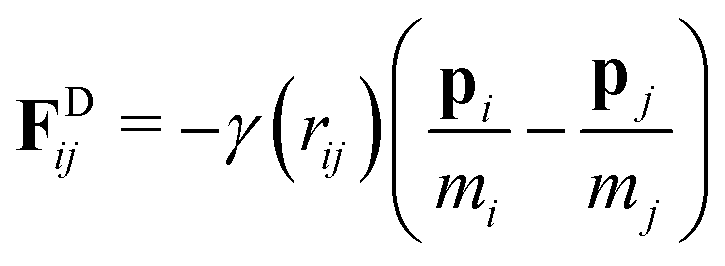
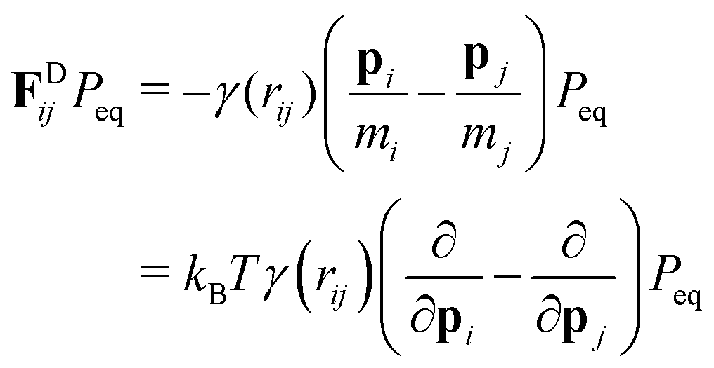

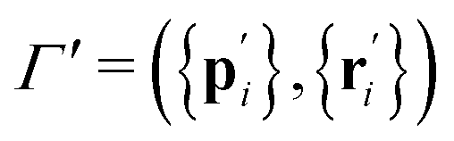 and is calculated according to the following algorithm:
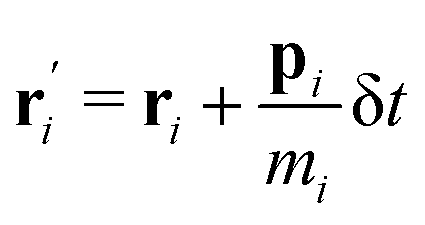
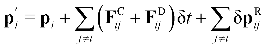
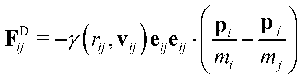
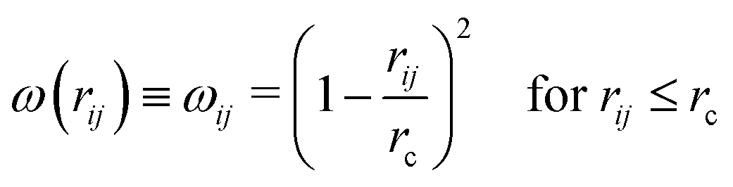
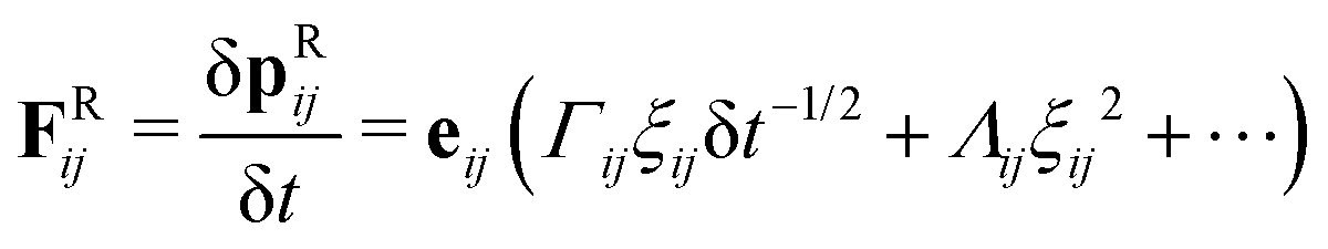
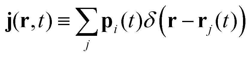
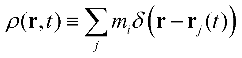

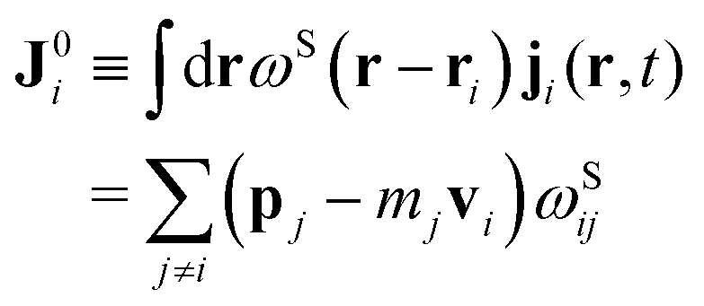
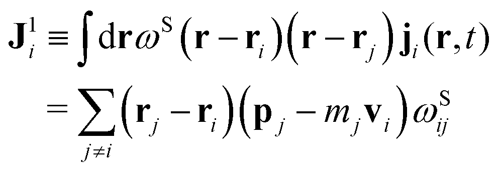
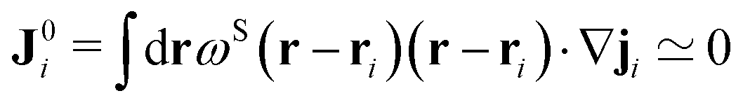
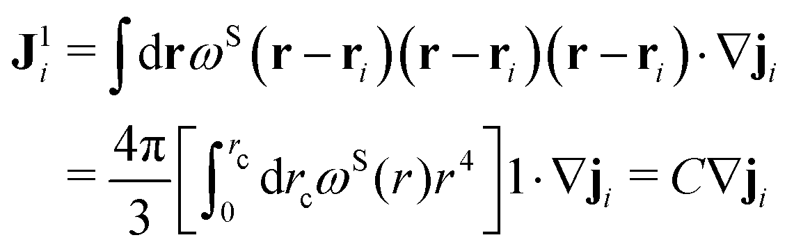
 and the geometric factor C, which depends on the mathematical expression for the kernel ωS. Therefore, comparing eqn (19) with eqn (22), we can estimate the local momentum gradient, i.e.,
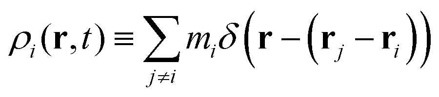
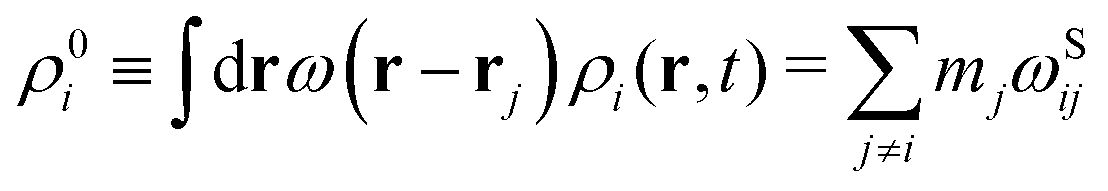

 in eqn (26) is multibody, which breaks the pairwise additiveness of the friction forces that is central in the DPD model. Therefore, rather than implementing the estimator as indicated in eqn (26), here we introduce a simplified version involving only pairwise contributions. Although this may seem very restrictive, is sufficient for the purpose of the article that is to show the modifications needed for the standard DPD equations for non-linear situations. Therefore, we choose this simplified model as is sufficient to meet this purpose. Effectively, we decompose
  into pairwise contributions
 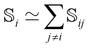 , with
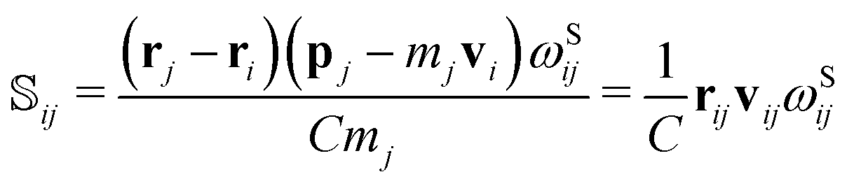
 is the antisymmetric tensor, where the superindex T stands for transpose, and we have chosen ωSij = θ(rc − rij). The quantity |rij × vij| is a measure of the rate of the local shearing motion of the particles i and j. However, as constructed, one cannot distinguish between the pure deformation of the local environment of particle i from a pure rigid body rotation of the same environment. To construct such estimator more than two particles are required, as it is expressed by eqn (25). For bounded flows, as in the Couette geometry that we explore in this article, neither free interfaces nor pure rotations are present and the use of such a simplified estimator for the shear rate is pertinent.
 stands for the trace of
  . For the same reasons expressed before, this estimator cannot distinguish a pure deformation of the volume element from a variation in its volume. The overlapping of these two modes of motion has been recently discussed in the context of other Lagrangian methods like SPH.18,32
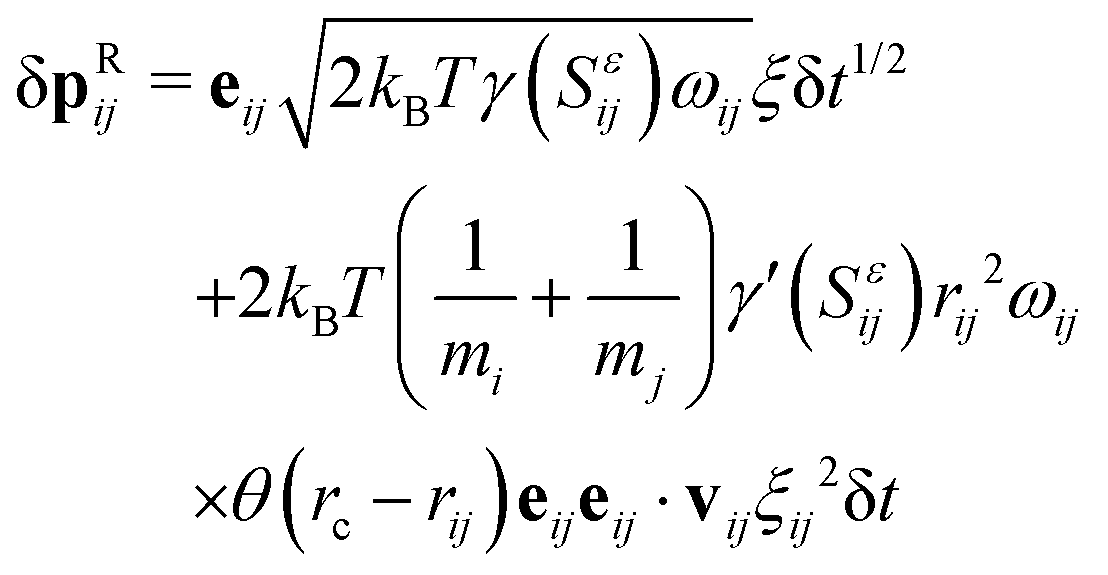
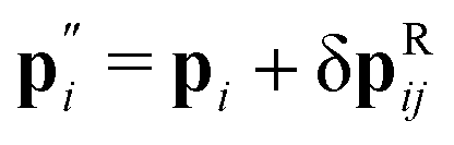

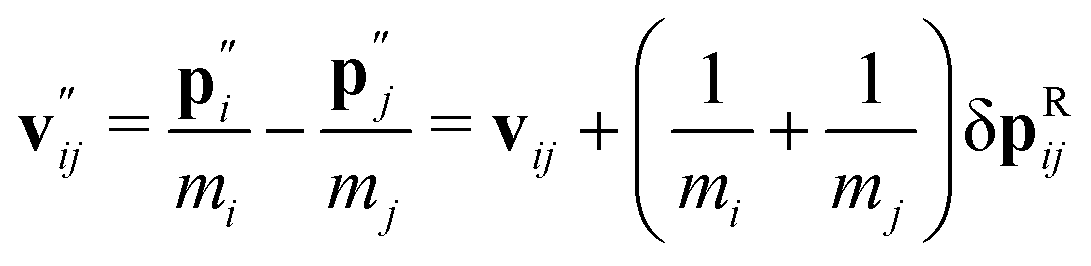
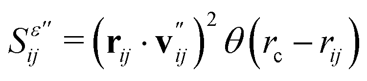
 is then calculated as,
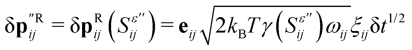
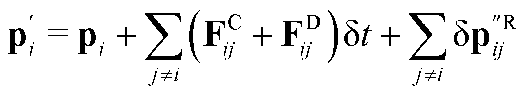
 is actually identical to the right-hand side of eqn (32), up to the order of validity of the algorithm,
  . We start by expanding eqn (37) up to first order in
  , i.e.,

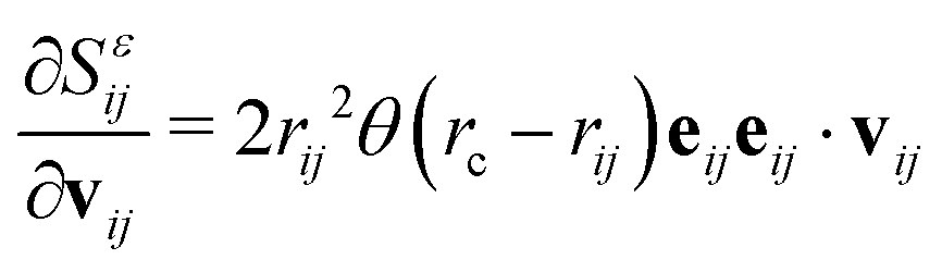
 , substituting eqn (40) and (41) into eqn (39) we arrive at,
 and for the subsequent calculation of the total random term δpRij.
 with all the other variables kept constant. In the spirit of Onsager's theory of non-equilibrium thermodynamics, one writes,
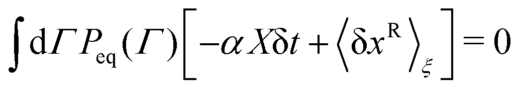
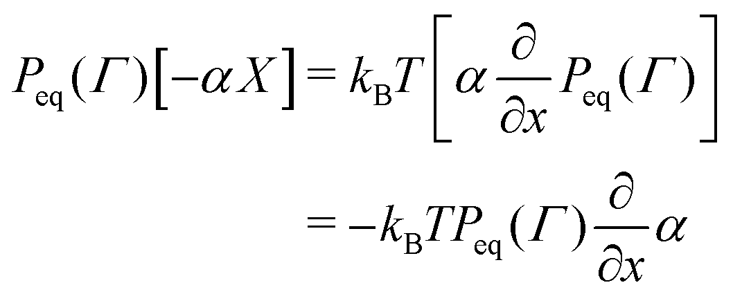
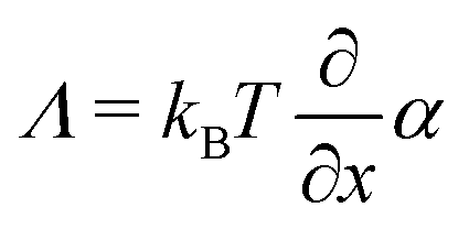
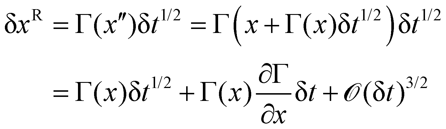

 , Q.E.D.
 . Using these scales from our reference system, we choose the mass of the DPD particle to be m = 1. We will analyse two different densities, namely n = 16 and n = 32. The dimensionless volume of the system corresponding to n = 16 is V = 1250, while for density n = 32, we selected V = 625. For equilibrium simulations, the box is cubic, with lateral sizes L = 10.77 and L = 8.55 for n = 16 and n = 32, respectively. For N-EQ simulations, the size on the x-direction is Lx = 2L while Ly = Lz = L. Therefore, V = 2L3, which gives L = 8.55 and L = 6.79 for the two densities. Moreover, the dimensionless temperature of our simulated system is 0.1, corresponding to a physical temperature T = 0.1u/kB, should we set the physical value of u. This temperature is used in the random force of the algorithm in all equilibrium and non-equilibrium simulations in this article. The chosen set of parameters does not necessarily correspond to any physical state of the reference system. The selection of the appropriate time-step δt = 10−4 is carefully considered and validated in Appendix B, using the measure of the viscosity to set the appropriate value. Periodic boundary conditions are applied in all three spatial coordinates. The thermalisation induced by the random force physically represents the coupling of the system with a heat reservoir at the same nominal temperature T. However, in the non-equilibrium simulations (cf. Section 3.3), we inject energy into the system, due to the momentum push at each slab, which eventually drains into the reservoir through the dissipative forces. Due to this phenomenon, kinetic temperatures that differ from the nominal temperature of the random force are observed at high rates of strain.
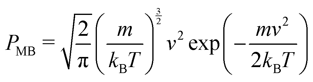
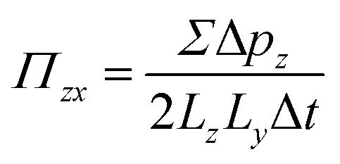
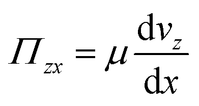
 (the latter, in dimensionless units). For the problem that we are addressing, this difference is not enough to produce high shear rates. We have thus introduced a variation in the original PeX method replacing the virtual collision by simply adding +Δpz to the selected particle with minor vz in slab 1 and −Δpz to that with major vz in slab 2 every δt, with no restriction on the size of Δpz. Although the total momentum conservation is maintained, the energy is not, as the procedure effectively pumps kinetic energy into the system. In the steady state, such energy influx is eventually dissipated by the friction forces, but the kinetic temperature of the system is therefore affected by the viscous heating. For each model and density, we have considered several cases characterised by a momentum Δpz transferred at every time-step, as indicated in Tables from 3 to 7. The resulting velocity profile, vz(x), is determined by dividing the whole box in the x-direction into 40 bins. At given instants of time, a snapshot of the system is taken and the z-component of the velocity field is obtained from the following average over the bin,
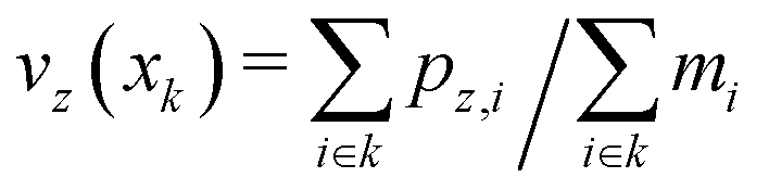
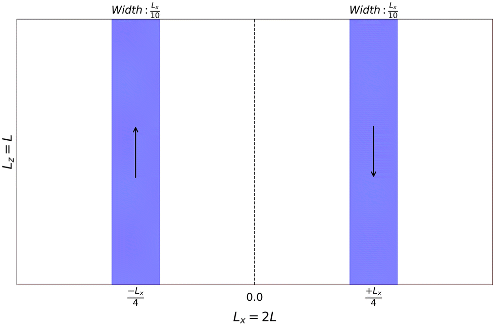
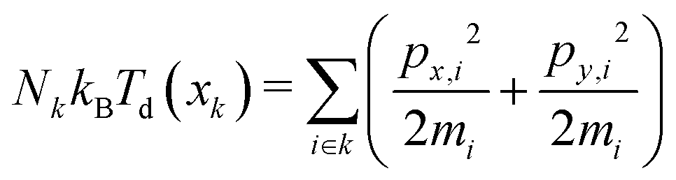
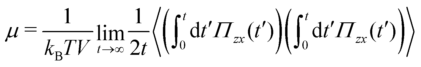
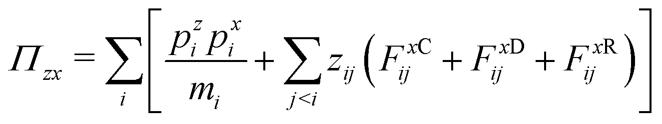
 used to correct the spurious contributions due to the non-linear friction. This fact is in agreement with the mechanistic interpretation of the stress tensor given in ref. 31. For the two-step algorithm, the contribution of FRij to the stress is calculated using the value of the random force after the first step.
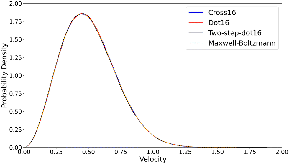

 , the non-linear models show a decreasing viscosity, while the reference cases do not. The slight increase of the viscosity in the reference linear case is also observed in Ref32. In Fig. 5 we have plotted the variation of the dynamic temperature as a function of the viscous heating. The plot shows a rather linear dependence of the temperature with the dissipation rate calculated at the centre of the box. We have included the cases Dot16 and the Two-step-dot16 to show that the increase of the temperature is the steepest. Due to this effect, there is no range within which a shear-thinning behaviour can be observed. In general, from Fig. 5 we can conclude that for the DPD models analysed the dynamic temperature varies inversely proportional to the actual value of the friction between the particles. Apart from the characteristic shear-thinning behaviour observable in the N-EQ simulations for both the Dot and Cross cases, we highlight that the two-step algorithm produces the same results for all properties measured in the simulations as found with the use of the standard algorithm with the random force eqn (32). Therefore, the corresponding plots in Fig. 4 closely follow each other.
 which creates local inhomogeneities in the velocity vz along the z-axis, namely δvz. We can consider that, at high shear rates, the motion of the kicked particle inside the slabs scatters the neighbouring particles, inducing a δvx component in localised places along the z-axis. In steady state, this effect is balanced by a gradient in pressure from the outer regions, to reach the mechanical equilibrium in the x direction. As this effect is mechanical, it is not reflected in the dynamic temperature of the slab. Hence, no local equilibrium can be properly defined. This consideration is very important to understand the nature of the inhomogeneities found during the simulations.
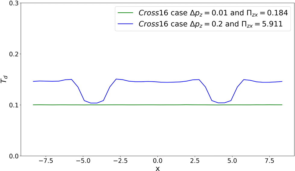
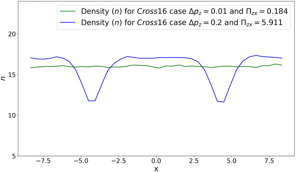

 and Γ*′ ≡ ({−pi}, {ri}). The change of sign depends on the parity under time reversal of the variable.16 Thus, detailed balance indicates that
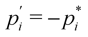 . Hence, the integration over Γ*′ can be readily performed. Using (63) we can write,
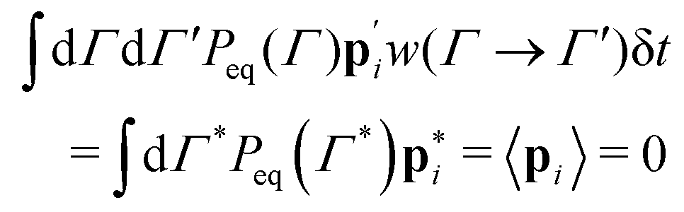

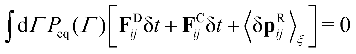
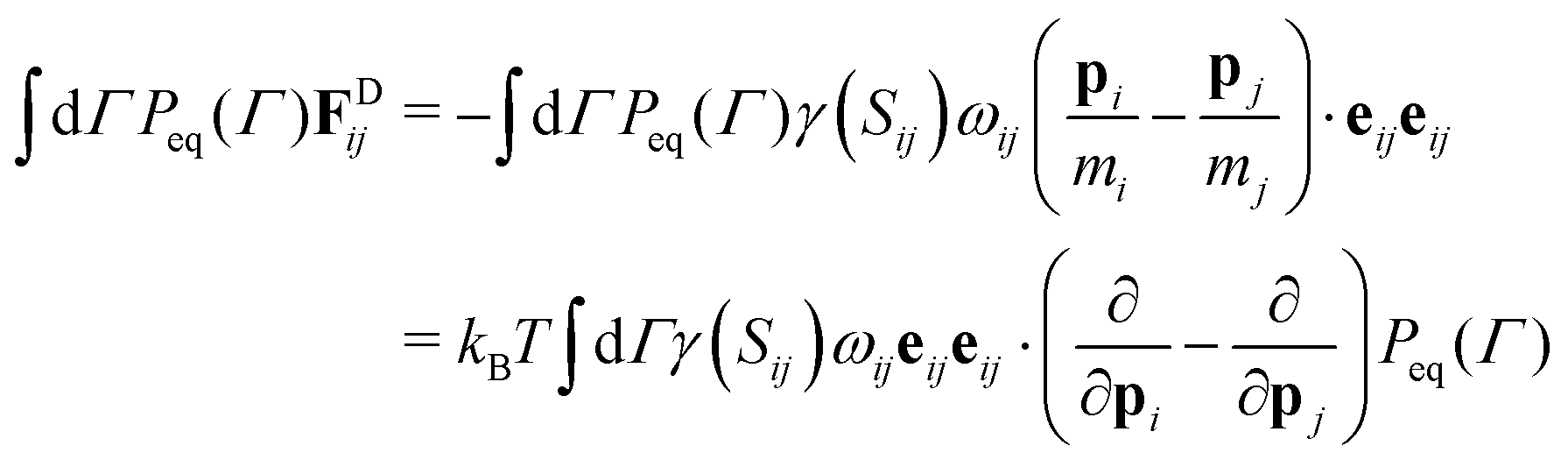
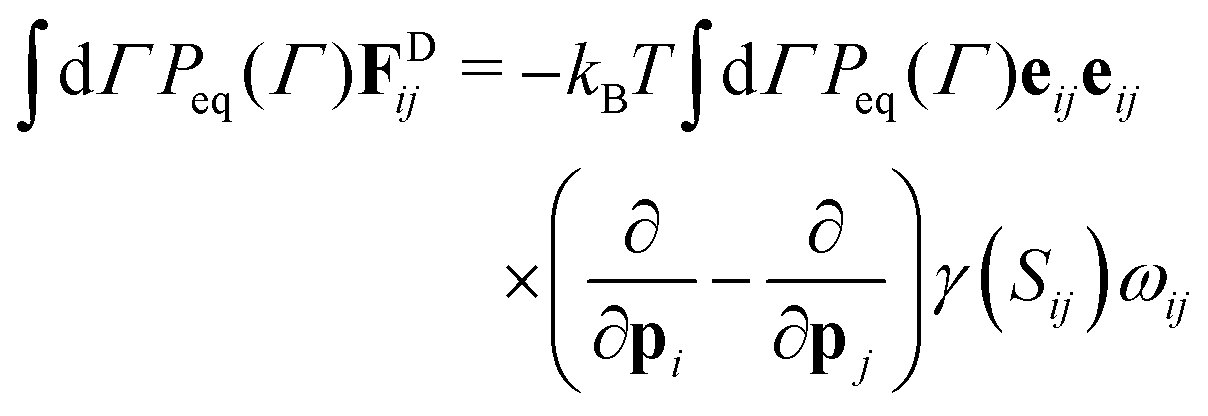
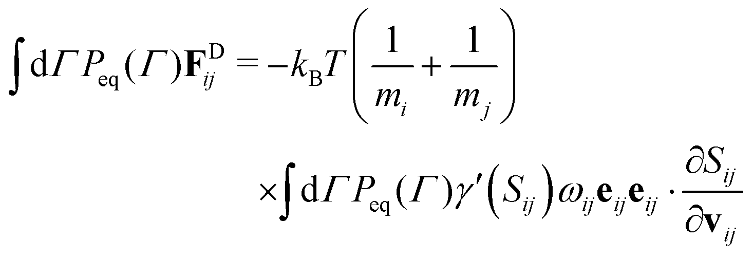
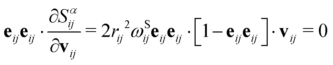
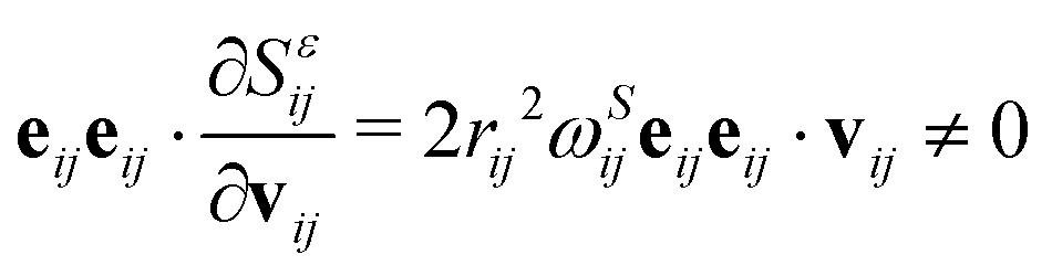


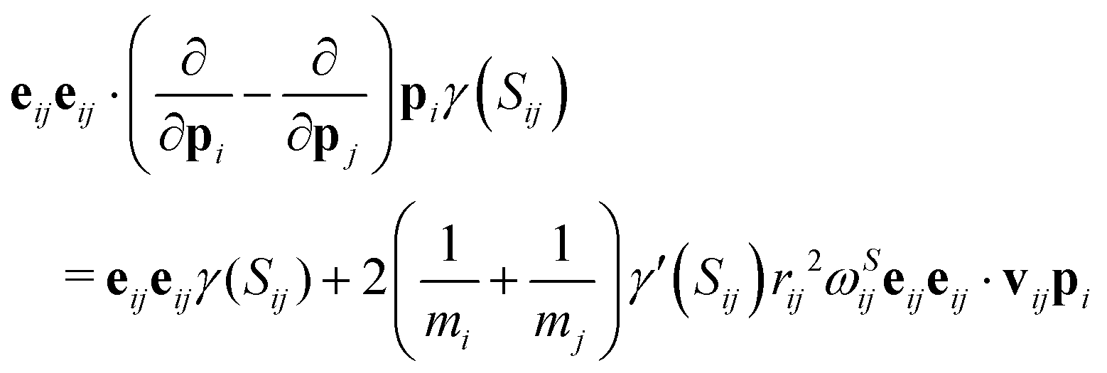
 , we can thus write