A non-Markovian neural quantum propagator and its application in the simulation of ultrafast nonlinear spectra
Received
28th September 2024
, Accepted 23rd November 2024
First published on 25th November 2024
Abstract
The accurate solution of dissipative quantum dynamics plays an important role in the simulation of open quantum systems. Here, we propose a machine learning-based universal solver for the hierarchical equations of motion, one of the most widely used approaches which takes into account non-Markovian effects and nonperturbative system–environment interactions in a numerically exact manner. We develop a neural quantum propagator model by utilizing the neural network architecture, which avoids time-consuming iterations and can be used to evolve any initial quantum state for arbitrarily long times. To demonstrate the efficacy of our model, we apply it to the simulation of population dynamics and linear and two-dimensional spectra of the Fenna–Matthews–Olson complex.
1 Introduction
Ultrafast nonlinear spectroscopy is a versatile tool to reveal the electronic structure and chemical reaction mechanism.1–5 Two-dimensional electronic spectroscopy (2DES), in particular, has been widely employed to monitor electronic excitation dynamics in polyatomic molecules.6–9 By utilizing multiple UV-Vis pulses, one can measure the correlation between different electronic states via off-diagonal peaks of 2DES. In addition, extracting dynamical information from the evolution of 2DES enables the direct visualization of chemical reaction processes.10–14
Theoretical simulation of nonlinear spectra is based on the response function theory, which requires the accurate description of system dynamics upon interaction with external laser pulses.15,16 As molecular systems inevitably interact with their surrounding environment, a commonly used strategy is to treat the environmental degrees of freedom as a heat bath and derive the equations of motion for the reduced system after tracing out bath degrees of freedom.17,18 The hierarchical equations of motion (HEOM) is one of the best-known quantum dynamics approaches, which takes into account non-Markovian effects and non-perturbative system–environment interactions in a numerically exact manner.19–21 As a typical differential equation, one recursively solves HEOM using conventional iterative solvers such as fourth-order Runge–Kutta (RK4) and split-operator methods.22–24 Despite their straightforward implementation, the main drawbacks of iterative methods are the large computational cost and long-time numerical instabilities. While improvements have been proposed to alleviate the numerical issues of iterative methods, an efficient universal solver is still to be proposed.25–27
Over recent years, the fast development of a machine learning technique offers new possibilities to circumvent aforementioned difficulties.28,29 A variety of machine learning based surrogate models have been developed to provide universal solvers for differential equations.30–33 In contrast to iterative methods, these surrogate models solve the differential equations by defining a functional that describes the mapping between an arbitrary initial condition and its corresponding solution at some subsequent time. This functional is then parameterized as a deep neural network and optimized with a prepared dataset. The state-of-the-art surrogate models, such as Fourier neural operator (FNO) and DeepONet, have shown their effectiveness over conventional methods on a set of classical dynamical problems.34–36
In this work, we extend the surrogate models to the non-Markovian quantum dynamics by developing a so-called neural quantum propagator (NQP) model for HEOM. As the quantum analogue of the universal solver for differential equations, the NQP model can be used to evolve any initial quantum state for arbitrarily long times. This universality renders its broader applications over other machine-learning-based dynamics solvers, which are mainly limited to the simulation of population dynamics.37–41 Following our previous work, we adopt the FNO architecture as the core neural network structure.42 We test its performance by comparing with the conventional RK4 method in various computational scenarios. In addition to the simulation of population dynamics, we also employ the NQP model to compute linear and nonlinear spectra.
Similar to other neural network architectures, the training NQP model requires a large amount of high precision data. These data can only be generated by conventional iterative solvers with a small enough time step, which in turn leads to a large computational cost in the data preparation stage. To address this issue, we introduce a super-resolution algorithm, which only relies on the low-resolution data to construct a high-resolution NQP model. The intrinsic error in the dataset is systematically improved by utilizing the physics-informed loss function (PILF), which is defined directly from the HEOM. The optimization of PILF does not rely on any prepared dataset, which significantly improves the overall computational performance of the NQP model.
The rest of the paper is organized as follows. In Section 2, we introduce the HEOM approach and linear and nonlinear response functions. In Section 3, we present the NQP model, including the FNO architecture, the training setup, and the super-resolution algorithm. Numerical demonstrations on the Fenna–Matthews–Olson (FMO) system are presented in Section 4. Finally, conclusions are drawn in Section 5.
2 Methodology
2.1 HEOM approach
We consider an electronic system interacting with a set of heat baths. The total Hamiltonian can be written as follows:| | | Ĥtot = Ĥs + Ĥb + Ĥs–b. | (1) |
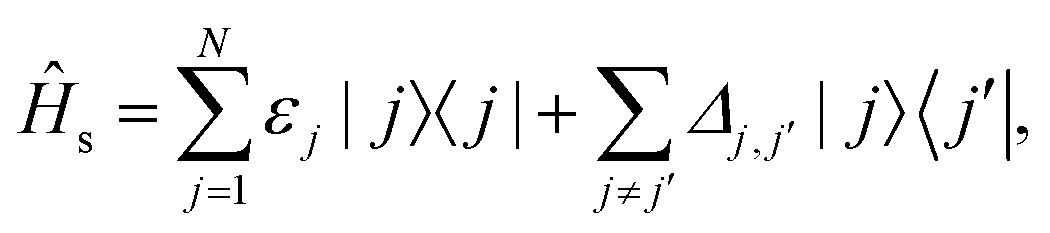
Here, the first term Ĥs is the Hamiltonian of the electronic system,| | 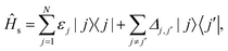 | (2) |
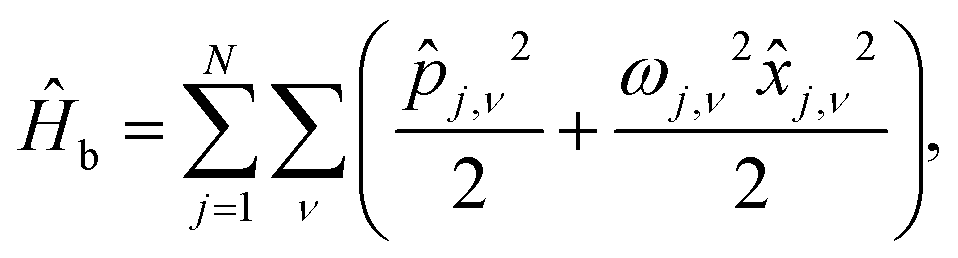
where εj is the energy of the jth electronic state |j〉, and Δj,j′ is the interstate coupling. The second term is the Hamiltonian of harmonic heat baths,| |  | (3) |
where ![[p with combining circumflex]](https://www.rsc.org/images/entities/i_char_0070_0302.gif) j,ν,
j,ν, ![[x with combining circumflex]](https://www.rsc.org/images/entities/i_char_0078_0302.gif) j,ν, and ωj,ν are the dimensionless momentum, coordinate, and frequency of νth oscillator of jth bath. The last term is the system–bath interaction Hamiltonian,
j,ν, and ωj,ν are the dimensionless momentum, coordinate, and frequency of νth oscillator of jth bath. The last term is the system–bath interaction Hamiltonian,| | 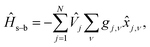 | (4) |
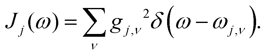
where ![[V with combining circumflex]](https://www.rsc.org/images/entities/i_char_0056_0302.gif) j = |j〉〈j|, and gj,ν is the coupling constant between the jth state and the νth oscillator which can be specified by a spectral density,
j = |j〉〈j|, and gj,ν is the coupling constant between the jth state and the νth oscillator which can be specified by a spectral density,| | 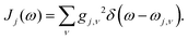 | (5) |
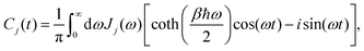
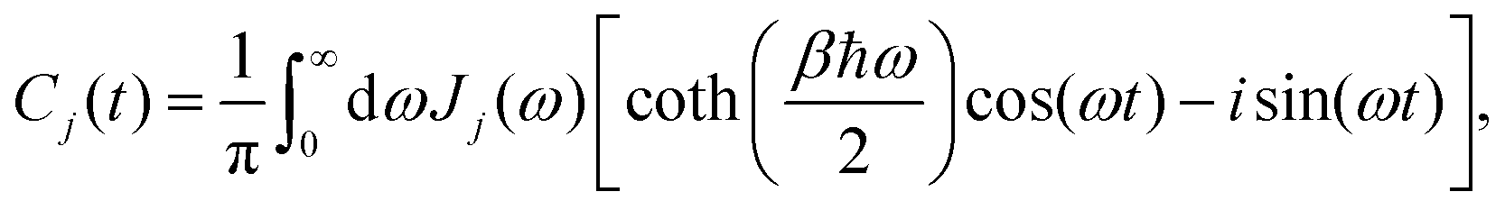
The influence of the jth heat bath on the electronic system is characterized by the bath correlation function,17,18
| |  | (6) |
where
Jj(
ω) is the spectral density of the
jth bath and
β = 1/
kBT is the inverse temperature with
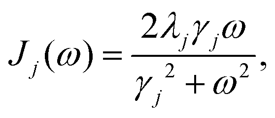
kB being the Boltzmann constant. We model the bath using the Drude spectral density,
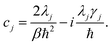
| |  | (7) |
where
λj is the reorganization energy and
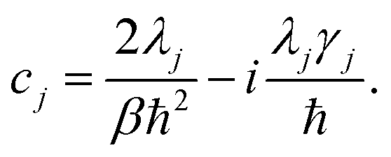
γj is the inverse of the bath correlation time. In this paper, we consider the high-temperature approximation (
βħγj < 1) and express
eqn (6) as
Cj(
t) =
cje
−γj|t|, where
| |  | (8) |
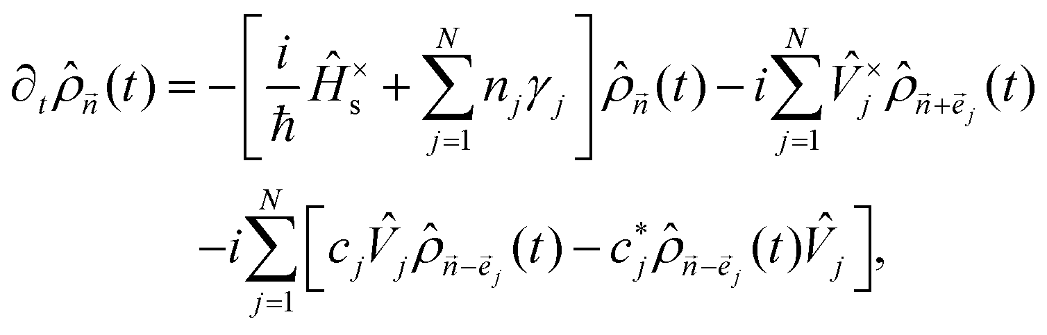
To go beyond this approximation, one can include so-called low-temperature correction terms.
43,44 The time evolution of the reduced density matrix can be described using the HEOM approach, which is written as follows:
19,45| | 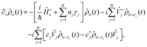 | (9) |
where
![[n with combining right harpoon above (vector)]](https://www.rsc.org/images/entities/i_char_006e_20d1.gif)
= {
n1,
n2,…,
nN} denotes the index vector with
nj being the non-negative integer, and we have introduced abbreviated notations,
Â×![[B with combining circumflex]](https://www.rsc.org/images/entities/i_char_0042_0302.gif)
=
 −
Â. The density operator with all indexes equal to zero,
![[small rho, Greek, circumflex]](https://www.rsc.org/images/entities/i_char_e0b7.gif)
![[0 with combining right harpoon above (vector)]](https://www.rsc.org/images/entities/char_0030_20d1.gif)
(
t) with
= {0, 0,…,0}, corresponds to the density operator of the reduced electronic system, while all other density operators are introduced to describe non-Markovian and non-perturbative effects.
2.2 Linear and nonlinear response functions
The linear and nonlinear spectra are evaluated within the framework of response function theory.1,16,46 The linear response function is defined as follows:| | 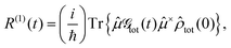 | (10) |
where ![[small mu, Greek, circumflex]](https://www.rsc.org/images/entities/i_char_e0b3.gif) is the transition dipole operator, and tot and
is the transition dipole operator, and tot and 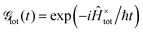 are the density operator and the quantum propagator of the total system, respectively. The linear absorption spectrum is obtained by the Fourier transformation:
| | 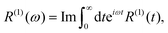 | (11) |
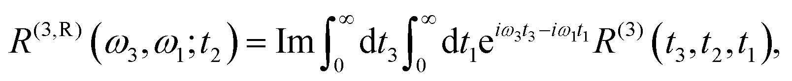
where Im denotes the imaginary part. The third-order response function is defined as follows:| | 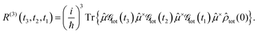 | (12) |
The rephasing and non-rephasing parts of the 2D spectrum are defined by:| | 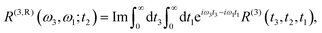 | (13) |
| | 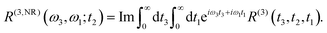 | (14) |
Within the HEOM formalism, eqn (10) and (12) can be evaluated by replacing tot and ![[capital G, script]](https://www.rsc.org/images/entities/char_e112.gif) tot(t) with (0) and eqn (9), respectively. The final trace is only taken for the zeroth order element of (t), i.e., (t).
tot(t) with (0) and eqn (9), respectively. The final trace is only taken for the zeroth order element of (t), i.e., (t).
3 Neural quantum propagator
We introduce the abbreviated index, x = (j,j′,n1,n2,…,nN), and align the matrix entries ρ(x,t) = 〈j|(t)|j′〉 as the column vector| | ![[small rho, Greek, vector]](https://www.rsc.org/images/entities/i_char_e137.gif) t = {ρ(x0,t),ρ(x1,t),…}. t = {ρ(x0,t),ρ(x1,t),…}. | (15) |
The HEOM (eqn (9)) can be recast to a matrix-vector form as:| | | ∂tt = Lt, | (16) |
where the matrix entries of L can be inferred from the right-hand side of eqn (9). The propagator of the HEOM is then defined through the integration form as Gt = exp(tL), which satisfies the composition property,| | | t = Gt−t0t0 = e(t−0)L. | (17) |
To facilitate the description of later sections, we also introduce a uniform time grid as tm = mδt for m = 1 ∼ Nt, where δt = tmax/Nt is the time step with Nt and tmax being the total number of time steps and the fixed upper time limit, respectively.
3.1 Model's architecture
The NQP model serves as an extension of the FNO to the quantum dynamics. Its mathematical foundation is the extended universal approximation theorem, which states that the large enough neural network can approximate the functional, representing the mapping between input and output pairs.47 To construct the NQP model, we follow our previous work42 and parameterize the HEOM propagator as a deep neural network, Gtm[θ], where θ represents all the trainable parameters. The architecture of the NQP model is shown in Fig. 1. In Fig. 1(a), the inputs are all entries of an initial state 0 and a specific time t, while the output is the corresponding solution t. The core part is called the Fourier layers with their structure presented in Fig. 1(b). Within Fourier layers, each entry is associated with several hidden channels. Pin and Pout are the linear projections between physical and latent Fourier spaces. They are parameterized as a point-wise convolution network with one hidden layer and a Gaussian error linear unit (GeLU) activation function.
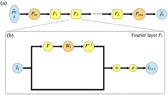 |
| | Fig. 1 The architecture of (a) the NQP model and (b) the lth Fourier layer. Here, ![[scr F, script letter F]](https://www.rsc.org/images/entities/char_e141.gif) and −1 denote the Fourier transform and its inverse. + and σ represent the element-wise sum and the GeLU activation function. The learnable parameters are those in Pin, Pout, and Wl. and −1 denote the Fourier transform and its inverse. + and σ represent the element-wise sum and the GeLU activation function. The learnable parameters are those in Pin, Pout, and Wl. | |
To process the input of the lth layer ![[v with combining right harpoon above (vector)]](https://www.rsc.org/images/entities/i_char_0076_20d1.gif) l, two different routes are adopted. On the upper route, and −1 denote the Fourier and its inverse transform. The point-wise convolution Wl serves as the learnable weight in Fourier space. Only the lowest kmax modes are explicitly included in the weight tensor, while others with higher frequencies are truncated to control the size of the model and avoid the numerical instabilities. The lower route is similar to the residual network. The results of two different routes are summed and activated by GeLU before passing to the next layer.
l, two different routes are adopted. On the upper route, and −1 denote the Fourier and its inverse transform. The point-wise convolution Wl serves as the learnable weight in Fourier space. Only the lowest kmax modes are explicitly included in the weight tensor, while others with higher frequencies are truncated to control the size of the model and avoid the numerical instabilities. The lower route is similar to the residual network. The results of two different routes are summed and activated by GeLU before passing to the next layer.
It should be noted that no restrictions are a priori made on the explicit forms of 0. The NQP model can be directly applied to the simulation of response functions by taking the field interaction form × as the input. Since the composition property is also retained during the parameterization, the time evolution up to arbitrarily long times can be obtained by recursively applying eqn (17).
3.2 Training objective
The NQP model is trained by minimizing an objective function ![[script L]](https://www.rsc.org/images/entities/char_e144.gif) , defined as follows:
, defined as follows:| | | = αdata + (1 − α)phys, | (18) |
where data and phys are referred to as the data and physics-informed loss functions, respectively. The hyper-parameter α ∈ (0,1) serves as a weight factor, which will be dynamically adjusted in the training stage.
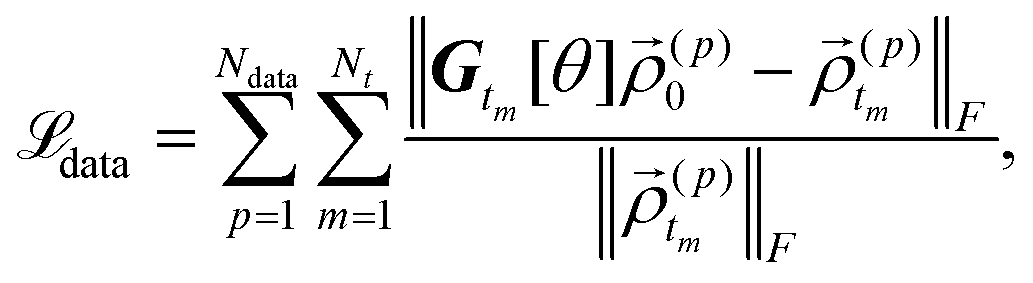
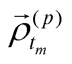
For the data part data, we prepare a dataset by randomly sampling a set of initial condition {0}, and then evaluating their time evolution {t} up to t ∈ [0,tmax] using the conventional RK4 method. The data loss function is defined as follows:
| | 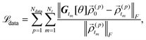 | (19) |
where ||·||
F denotes the Frobenius-norm,
Ndata is the number of individual samples in the dataset, and
(p)0 and

are the initial condition and the corresponding evolution for the
pth sample, respectively.
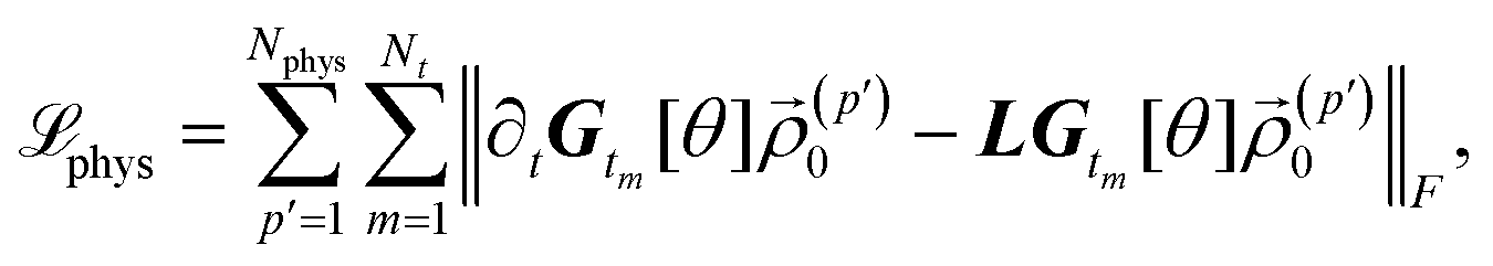
To ensure the universality of Gt[θ] that is applicable to any 0, one needs a large number of samples Ndata, which leads to even more computational cost in the data preparation stage. We introduce a physics-informed loss function to reduce the effective number of samples Ndata while keeping the universality of Gt[θ].48 The physics-informed loss function is defined by minimizing the difference between left- and right-hand sides of eqn (16) as:
| | 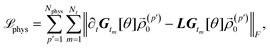 | (20) |
where
Nphys is the number of samples in the physics dataset. The time derivative ∂
tt is evaluated using the finite difference method. It should be mentioned that the calculation of
phys involves far less samples as compared to that of
data. In addition, we adopt the on-the-fly sampling approach by re-generating the physics dataset at each training epoch to further improve the performance of the trained model.
3.3 Super resolution algorithm
To further reduce the computational cost in the data preparation stage, we introduce a super resolution algorithm, which allows the construction of the high resolution NQP model from a lower resolution dataset. As illustrated from the previous subsection, the lower resolution dataset is prepared by integrating the HEOM with a larger time step Kδt (K > 1) for a set of {0} using the RK4 method. The obtained data are then embedded into the finer grid {tm = mδt} by interpolating the missing value using the linear interpolation scheme. data is evaluated on this interpolated dataset in the training stage.
On the other hand, the physics-informed loss function phys is evaluated directly on the finer time grid and serves as the correction over the deviation from the dataset. The super resolution algorithm is then completed by dynamically adjusting the weight factor α in eqn (18) during the training process. At the beginning, we set α = 1 and randomly initialize all the model's parameters. During the training process, α is gradually decreased to a small enough value such as ∼0.01, and phys gradually becomes the dominant contribution term. The minimization of phys allows the improvement of the resolution over the intrinsic deviation of the dataset.
At the end of this subsection, we briefly discuss the possibility of data-free training, which is achieved by fixing α = 0 and using only phys during the training process. From a theoretical point of view, training with or without data results in the same model as long as phys becomes the dominant contribution of eqn (18). In practice, however, training with only phys requires longer epochs for convergence when all the learnable parameters are randomly initialized. In this case, a prepared dataset, even with low resolution, provides effective guidance for the training process.
4 Numerical experiments
In the following, we use the seven-site FMO-complex (apo-FMO) as the model system and adopt the Adolph and Renger's Hamiltonian.49,50 We restrict the discussion to the one-exciton manifold. The electronic state |j〉 (j = 1,…,7) corresponds to the state where only the jth pigment is excited, and |g〉 denotes the ground state without any excitation. The system–bath interaction is chosen as j = |j〉〈j| and g ≡ 0. The heat bath parameters are chosen as λj = 35 cm−1, γj = 200 cm−1, and T = 300 K, respectively. The HEOM is truncated at the hierarchy level of  after adopting the filtering algorithm.51 Within our choice of parameters and under the high-temperature limit, we found that it is accurate enough for the testing of our NQP model. We set the upper time limit as tmax = 30 fs with a time step of δt = 0.6 fs, which results in Nt = 50 time points.
4.1 Training and validation test
We first introduce the model's hyper-parameters and training setup. In order to train the NQP model, we prepare the low-resolution training dataset by randomly sampling Ndata = 3000 initial conditions 0. The low resolution dataset is prepared by integrating HEOM with a larger time step of 3δt. The missing values are linearly interpolated when embedded into the finer grid with a time step of δt. To test the accuracy of the model, we also prepare a high-resolution validation set with 500 samples, following the same setup but using a smaller time step of δt. It should be noted that the high-resolution validation set is never used in the training stage. In the training process, the physics dataset is prepared using the on-the-fly sampling algorithm by randomly generating Nphys = 2000 initial conditions at each epoch.
The other hyper-parameters of the NQP model are chosen as follows. We set the hidden channel of projections Pin and Pout as 512. We use 4 Fourier layers, each of which has a hidden channel of size 64, and the total number of trainable parameters is around 10 million. The model is trained for 105 epochs using the Adam optimizer. The learning rate is initially set to 10−4, and then halved every 500 epochs until reaching 10−6. The weight factor α in eqn (18) is initialized as α = 1, and halved every 100 epochs until reaching ∼10−2. All the tasks are performed on the Nvidia A40 GPU with 48 GB memory and completed within 200 hours.
To test our model, we present the validation test by showing the relative error of data for each sample in the validation set in Fig. 2. For all samples, the relative error is around 0.5%. This error can be further reduced by using more samples in the data and physics sets, extending the training to longer epochs, and increasing the size of the NQP model. It should be pointed out that this error corresponds to the overall deviation of all the entries of , including those deep hierarchy elements that have a much smaller magnitude as compared to .
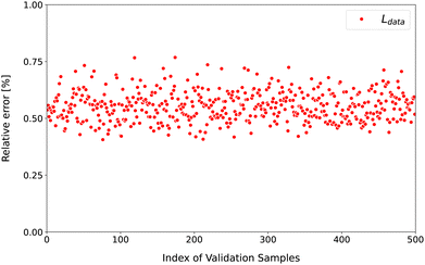 |
| | Fig. 2 The relative error of data for the validation set. The horizontal axis represents the index of the samples, while the vertical axis is the relative error. | |
4.2 Population dynamics
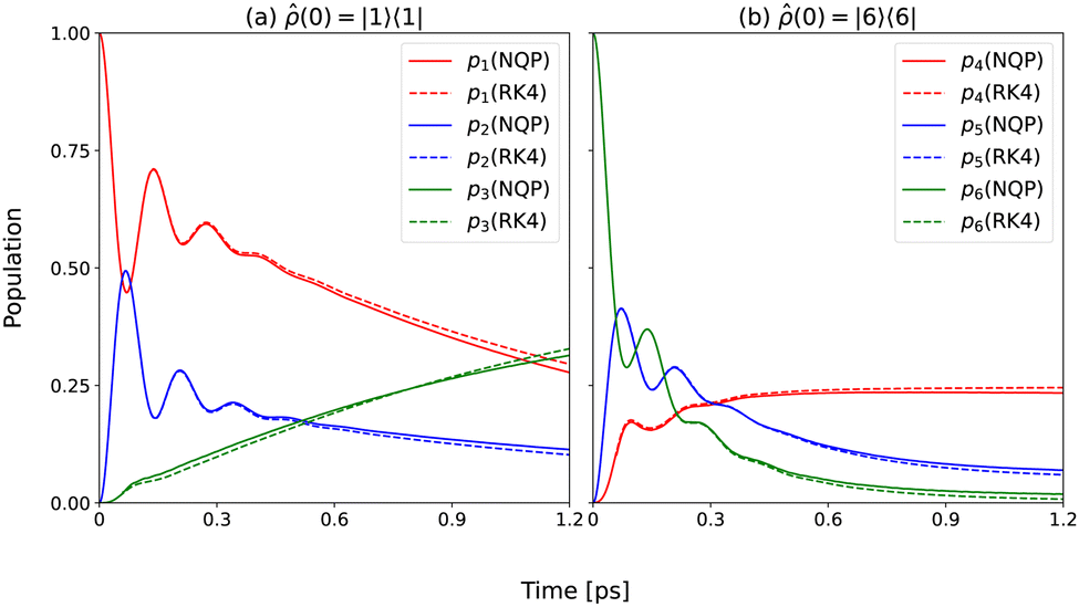
By using the composition property, t1+t2 = Gt2[θ]t1, our NQP model can accurately predict long-time dynamics well beyond the training time limit tmax. To test the accuracy of the long-time dynamics predicted using the NQP model, we compute population dynamics up to 40tmax (∼1.2 ps). The reference results are obtained from the RK4 method with an integration time step of δt. Here, we consider two initial conditions: (a) (0) = |1〉〈1|, and (b) (0) = |6〉〈6|, which correspond to the excitation localized at the first and sixth pigments, respectively. All other hierarchy elements (0) ( ≠ ) are set to zero for the factorized bath initial condition.
In Fig. 3, we show the time evolution of populations pn(t) = 〈n|(t)|n〉 for sites (a) n = 1, 2, and 3 and (b) n = 4, 5, and 6, respectively, following the experimentally demonstrated energy transfer pathways. In both cases, our NQP model yields results in good agreement with those from the reference RK4 method up to 10tmax. While model-predicted long time dynamics deviates slightly from the exact results due to the accumulation of errors in the training stage, our NQP model still infers the accurate dynamics even far beyond the training time (40tmax).
 |
| | Fig. 3 Population dynamics computed using the NQP model (solid lines) and the reference RK4 method (dashed lines) for two typical initial conditions up to t = 1.2 ps (40tmax). | |
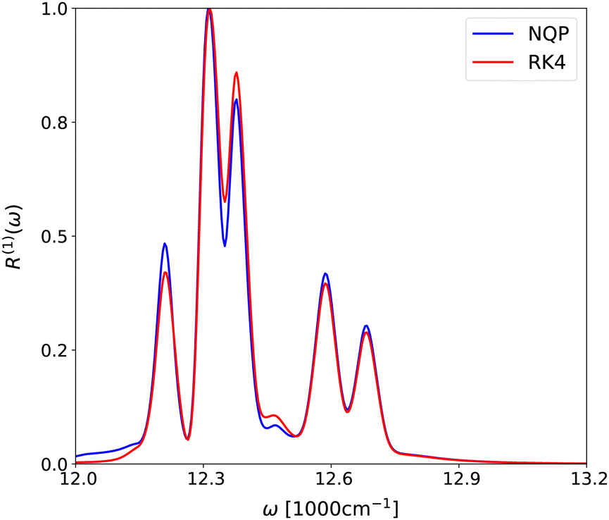
4.3 Linear spectra
Next, we apply our NQP model to simulate the linear and third-order response functions as defined in eqn (10) and (12). We choose the transition dipole operator as:| |  | (21) |
where μj is the transition dipole moment of jth pigment. The system is initially in the electronic ground state before the photoexcitation, i.e., (0) = |g〉〈g|.
In Fig. 4, we show the linear spectrum evaluated from the NQP model and the RK4 method. For each case, we set the time window of t to [0,40tmax], and normalize the peak intensities with respect to their own maximum value. Overall, the NQP model yields the spectrum in good agreement with that from the reference RK4 method. The small deviations of some peak intensities may be attributed to the model's architecture. The adaption of Fourier transform in the model's architecture generates some artificial aliasing modes, the magnitudes of which are increased after recurrent evaluation of long time dynamics. This systematic error could be resolved by carefully fine tuning the truncation level of Fourier modes in the NQP model, or by replacing the Fourier transform with methods such as wavelet transform or spatial convolutions.
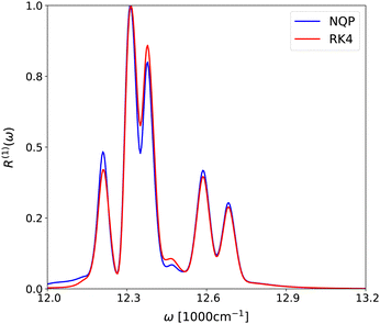 |
| | Fig. 4 The linear spectrum R(1)(ω) evaluated from the NQP model (blue line) and the RK4 method (red line), respectively. | |
4.4 Two-dimensional spectra
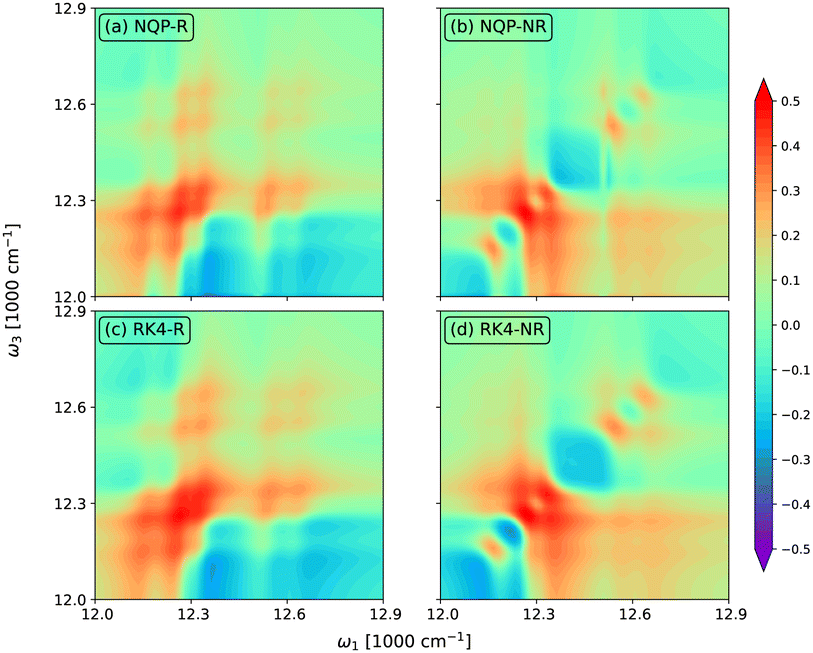
We further apply the NQP model to compute 2D spectra at different time t2. Since we restrict the discussion to the one-exciton manifold, the two-exciton states, which contribute to the excited-state absorption of 2D spectra, are not included in the Hamiltonian. The simulated 2D spectra thus only involve the contribution of ground-state bleach and stimulated emission. The inclusion of two-exciton states can be easily established by adding the electronic states |jj′〉, which represent the simultaneous excitation at two pigments, to the Hamiltonian, and increasing the length of the column vector t defined in eqn (15). The NQP model can handle this expanded system by using more layers and increasing the size of each layer. However, this will require more learnable parameters and lead to a dramatic increase of the computational cost especially in the training stage, which is outside the scope of the present work.
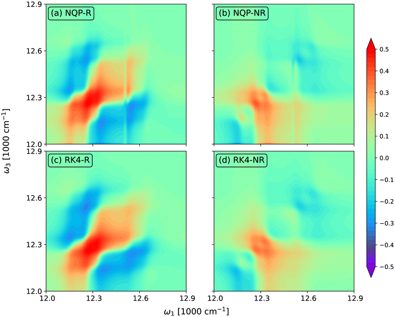
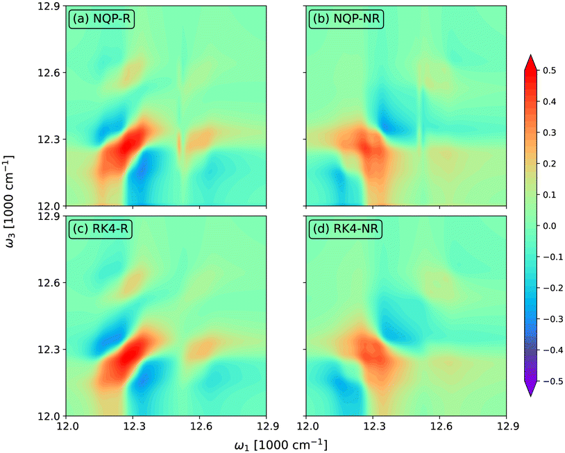
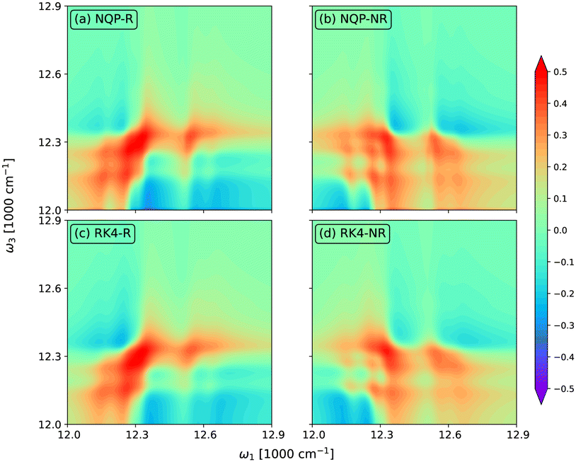
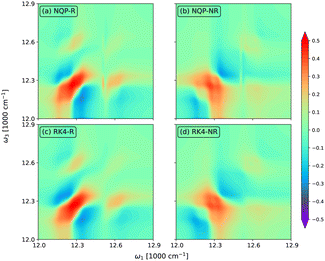
In Fig. 5, we show the rephasing (a) and (c) and non-rephasing (b) and (d) parts of 2D spectra at t2 = 0 fs evaluated from the NQP model (a) and (b) and the RK4 reference method (c) and (d), respectively. We set the time window of both t1 and t3 to [0,40tmax]. For better illustration, we adopt the widely used arcsinh scaling after the normalization of peak intensities.52–54 While the simulation of 2D spectra at t2 = 0 fs requires the propagation up to t1 + t3 ≤ 80tmax, far beyond the training time limit, both rephasing and non-rephasing parts of 2D spectra predicted by the NQP model are again in good agreement with those from the RK4 reference method, demonstrating the long-time reliability of our NQP model. The rephasing and non-rephasing parts of 2D spectra at t2 = 50, 100, and 500 fs evaluated from the NQP model and the RK4 reference method are shown in Fig. 6–8. The NQP model again yields accurate 2D spectra, illustrating the energy relaxation process from higher exciton states to lower exciton states as t2 increases.
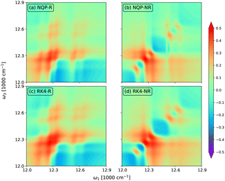 |
| | Fig. 5 2D spectra at t2 = 0 fs evaluated from (a) and (b) the NQP model and (c) and (d) the RK4 reference method, respectively. ‘R’ in (a) and (c) and ‘NR’ in (b) and (d) denote the rephasing and non-rephasing parts, respectively. | |
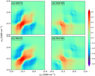 |
| | Fig. 6 The rephasing (a) and (c) and non-rephasing (b) and (d) parts of 2D spectra at t2 = 50 fs evaluated from (a) and (b) the NQP model and (c) and (d) the RK4 reference method, respectively. | |
 |
| | Fig. 7 The rephasing (a) and (c) and non-rephasing (b) and (d) parts of 2D spectra at t2 = 100 fs evaluated from (a) and (b) the NQP model and (c) and (d) the RK4 reference method, respectively. | |
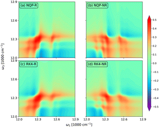 |
| | Fig. 8 The rephasing (a) and (c) and non-rephasing (b) and (d) parts of 2D spectra at t2 = 500 fs evaluated from (a) and (b) the NQP model and (c) and (d) the RK4 reference method, respectively. | |
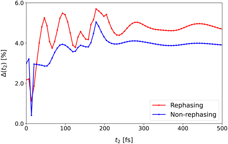
To quantify the difference between model-predicted and reference spectra more specifically, we define the averaged point-wise relative deviation as follows:
| |  | (22) |
where
Ω1,
Ω3 ∈ (12
![[thin space (1/6-em)]](https://www.rsc.org/images/entities/char_2009.gif)
000 cm
−1, 12
900 cm
−1),
R(3)NQP and
R(3)RK4 are the spectra evaluated from the NQP model and the RK4 reference method, respectively, and
ε ∼ 10
−6 is employed to avoid the numerical divergence. In
Fig. 9, we display Δ(
t2) up to
t2 = 500 fs with a time step of 20 fs. With the increase of
t2, the relative error also rapidly increases due to the fast relaxation of the system. After the system reaches the equilibrium, the error also reaches the plateau at around 4–5%. This again demonstrates the long-time reliability of our NQP model.
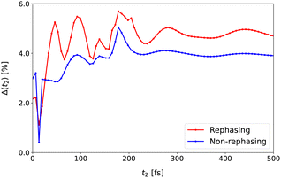 |
| | Fig. 9 The relative error between the NQP model and the RK4 reference method as a function of t2. | |
5 Conclusions
In this work, we develop a NQP model for the HEOM approach to treat the non-Markovian dynamics. We use the FNO as the model's architecture and design a super-resolution algorithm to reduce the computational cost in the data preparation stage. In the training stage, we employ both the data loss function and an extra PILF to improve the numerical performance. The accuracy of the NQP model is tested by computing the population dynamics and linear and two-dimensional spectra. The NQP model yields results in good agreement with the conventional RK4 method, demonstrating its potential applicability in various computational scenarios.
In the current NQP model, the number of learnable parameters scales exponentially with both the size of the reduced system and the number of hierarchy elements. To alleviate the computational cost, future work may extend the NQP model to deal with the decomposed form of (t). For example, (t) can be expressed as a matrix-product-state form by using the twin-space formulation and tensor-train decomposition, which requires far less entries than the original density matrix.55,56 In addition, our focus here is on the time-independent Hamiltonian. Future development may extend to the driven dynamics, where the system Hamiltonian contains time-dependent external fields. A typical application is the spectroscopic equations of motion approach which was employed for the simulation of strong-field nonlinear spectra with different pulse profiles.57,58 It is also interesting to extend our NQP model to be applicable to systems governed by different types of Hamiltonians. Work in these directions is in progress.
Data availability
The data that support the finding of this work are available at https://github.com/jiaji-zhang/Neural-Quantum-Propagator. The code for training ML models and generating population dynamics and spectra can be found at https://github.com/jiaji-zhang/Neural-Quantum-Propagator.
Conflicts of interest
The authors have no conflicts to disclose.
Acknowledgements
J. Z. and L. P. C. acknowledge support from the starting grant of research center of new materials computing of Zhejiang Lab (No. 3700-32601).
References
- M. F. Gelin, L. Chen and W. Domcke, Chem. Rev., 2022, 122, 17339–17396 CrossRef CAS PubMed.
- M. Nisoli, P. Decleva, F. Calegari, A. Palacios and F. Martín, Chem. Rev., 2017, 117, 10760–10825 CrossRef CAS PubMed.
- S. Mukamel, Annu. Rev. Phys. Chem., 2000, 51, 691–729 CrossRef CAS PubMed.
- M. Maiuri, M. Garavelli and G. Cerullo, J. Am. Chem. Soc., 2019, 142, 3–15 CrossRef PubMed.
- K. E. Dorfman, F. Schlawin and S. Mukamel, Rev. Mod. Phys., 2016, 88, 045008 CrossRef.
- E. Fresch, F. V. A. Camargo, Q. Shen, C. C. Bellora, T. Pullerits, G. S. Engel, G. Cerullo and E. Collini, Nat. Rev. Methods Primers, 2023, 3, 84 CrossRef CAS.
- T. A. A. Oliver, R. Soc. Open Sci., 2018, 5, 171425 CrossRef.
- G. S. Schlau-Cohen, A. Ishizaki and G. R. Fleming, Chem. Phys., 2011, 386, 1–22 CrossRef CAS.
- N. S. Ginsberg, Y.-C. Cheng and G. R. Fleming, Acc. Chem. Res., 2009, 42, 1352–1363 CrossRef CAS PubMed.
- G. D. Scholes, G. R. Fleming, A. Olaya-Castro and R. van Grondelle, Nat. Chem., 2011, 3, 763–774 CrossRef CAS.
- M. Kullmann, S. Ruetzel, J. Buback, P. Nuernberger and T. Brixner, J. Am. Chem. Soc., 2011, 133, 13074–13080 CrossRef CAS PubMed.
- E. A. Arsenault, P. Bhattacharyya, Y. Yoneda and G. R. Fleming, J. Chem. Phys., 2021, 155, 020901 CrossRef CAS PubMed.
- J. Kim, J. Jeon, T. H. Yoon and M. Cho, Nat. Commun., 2020, 11, 6029 CrossRef CAS.
- S. Ruetzel, M. Kullmann, J. Buback, P. Nuernberger and T. Brixner, Phys. Rev. Lett., 2013, 110, 148305 CrossRef PubMed.
-
M. Cho, Coherent Multidimensional Spectroscopy, Springer, Singapore, 2019 Search PubMed.
-
S. Mukamel, Principles of Nonlinear Optical Spectroscopy, Oxford University Press, 1995 Search PubMed.
-
H.-P. Breuer and F. Petruccione, The Theory of Open Quantum Systems, Oxford University Press, 2007 Search PubMed.
-
U. Weiss, Quantum Dissipative Systems, World Scientific, 4th edn, 2012 Search PubMed.
- Y. Tanimura, J. Chem. Phys., 2020, 153, 020901 CrossRef CAS.
- L. Ye, X. Wang, D. Hou, R. Xu, X. Zheng and Y. Yan, Wiley Interdiscip. Rev.:Comput. Mol. Sci., 2016, 6, 608–638 Search PubMed.
- J. Zhang and Y. Tanimura, J. Chem. Phys., 2022, 156, 174112 CrossRef CAS.
-
P. E. Kloeden and E. Platen, Numerical Solution of Stochastic Differential Equations, Springer, Berlin, Heidelberg, 1992 Search PubMed.
- Y. Yan, M. Xu, T. Li and Q. Shi, J. Chem. Phys., 2021, 154, 194104 CrossRef CAS.
- Y. Ke, J. Chem. Phys., 2023, 158, 211102 CrossRef CAS.
- A. Kimura and Y. Fujihashi, J. Chem. Phys., 2014, 141, 194110 CrossRef PubMed.
- A. W. Schlimgen, K. Head-Marsden, L. M. Sager, P. Narang and D. A. Mazziotti, Phys. Rev. Lett., 2021, 127, 270503 CrossRef CAS PubMed.
- W. Liu, Z.-H. Chen, Y. Su, Y. Wang and W. Dou, J. Chem. Phys., 2023, 159, 144110 CrossRef CAS PubMed.
- Y. LeCun, Y. Bengio and G. Hinton, Nature, 2015, 521, 436–444 CrossRef CAS.
- J. Hermann, J. Spencer, K. Choo, A. Mezzacapo, W. M. C. Foulkes, D. Pfau, G. Carleo and F. Noé, Nat. Rev. Chem., 2023, 7, 692–709 CrossRef PubMed.
- L. Lu, P. Jin, G. Pang, Z. Zhang and G. E. Karniadakis, Nat. Mach. Intell., 2021, 3, 218–229 CrossRef.
-
Z. Li, N. Kovachki, K. Azizzadenesheli, B. Liu, K. Bhattacharya, A. Stuart and A. Anandkumar, arXiv, 2021, 2010.08895 Search PubMed.
- N. Kovachki, Z. Li, B. Liu, K. Azizzadenesheli, K. Bhattacharya, A. Stuart and A. Anandkumar, J. Mach. Learn. Res., 2023, 24, 1–97 Search PubMed.
-
J. Guibas, M. Mardani, Z. Li, A. Tao, A. Anandkumar and B. Catanzaro, 2021, arXiv, 2111.13587 Search PubMed.
- L. Lu, X. Meng, Z. Mao and G. E. Karniadakis, SIAM Rev., 2021, 63, 208–228 CrossRef.
-
J. Pathak, S. Subramanian, P. Harrington, S. Raja, A. Chattopadhyay, M. Mardani, T. Kurth, D. Hall, Z. Li, K. Azizzadenesheli, P. Hassanzadeh, K. Kashinath and A. Anandkumar, 2022, arXiv, 2202.11214 Search PubMed.
-
P. Jiang, N. Meinert, H. Jordão, C. Weisser, S. Holgate, A. Lavin, B. Lütjens, D. Newman, H. Wainwright, C. Walker and P. Barnard, 2021, arXiv, 2110.07100 Search PubMed.
- J. Cerrillo and J. Cao, Phys. Rev. Lett., 2014, 112, 110401 CrossRef.
- K. Lin, J. Peng, F. L. Gu and Z. Lan, J. Phys. Chem. Lett., 2021, 12, 10225–10234 CrossRef CAS PubMed.
- L. E. Herrera Rodríguez and A. A. Kananenka, J. Phys. Chem. Lett., 2021, 12, 2476–2483 CrossRef PubMed.
- A. Ullah and P. O. Dral, New J. Phys., 2021, 23, 113019 CrossRef CAS.
- D. Wu, Z. Hu, J. Li and X. Sun, J. Chem. Phys., 2021, 155, 224104 CrossRef CAS PubMed.
- J. Zhang, C. L. Benavides-Riveros and L. Chen, J. Phys. Chem. Lett., 2024, 15, 3603–3610 CrossRef CAS PubMed.
- A. Ishizaki and Y. Tanimura, J. Phys. Soc. Jpn., 2005, 74, 3131–3134 CrossRef CAS.
- J. Hu, R.-X. Xu and Y. Yan, J. Chem. Phys., 2010, 133, 101106 CrossRef.
- Y. Tanimura, J. Phys. Soc. Jpn., 2006, 75, 082001 CrossRef.
- J. Zhang and Y. Tanimura, J. Chem. Phys., 2023, 159, 014102 CrossRef CAS.
- N. Kovachki, S. Lanthaler and S. Mishra, J. Mach. Learn. Res., 2021, 22, 1–76 Search PubMed.
- S. G. Rosofsky, H. A. Majed and E. A. Huerta, Mach. Learn.: Sci. Technol., 2023, 4, 025022 Search PubMed.
- J. Adolphs and T. Renger, Biophys. J., 2006, 91, 2778–2797 CrossRef CAS PubMed.
- A. Ishizaki and G. R. Fleming, Proc. Natl. Acad. Sci. U. S. A., 2009, 106, 17255–17260 CrossRef.
- Q. Shi, L. Chen, G. Nan, R.-X. Xu and Y. Yan, J. Chem. Phys., 2009, 130, 084105 CrossRef PubMed.
- S.-H. Yeh and S. Kais, J. Chem. Phys., 2014, 141, 234105 CrossRef PubMed.
- L. Chen, R. Zheng, Y. Jing and Q. Shi, J. Chem. Phys., 2011, 134, 194508 CrossRef PubMed.
- M. Cho, H. M. Vaswani, T. Brixner, J. Stenger and G. R. Fleming, J. Phys. Chem. B, 2005, 109, 10542–10556 CrossRef CAS PubMed.
- R. Borrelli, J. Chem. Phys., 2019, 150, 234102 CrossRef.
- R. Borrelli and M. F. Gelin, Wiley Interdiscip. Rev.: Comput. Mol. Sci., 2021, 11, e1539 CAS.
- H. Wang and M. Thoss, Chem. Phys. Lett., 2004, 389, 43–50 CrossRef CAS.
- H. Wang and M. Thoss, Chem. Phys., 2008, 347, 139–151 CrossRef CAS.
|
| This journal is © the Owner Societies 2025 |
Click here to see how this site uses Cookies. View our privacy policy here. 
 * and
Lipeng
Chen
* and
Lipeng
Chen


 are the density operator and the quantum propagator of the total system, respectively. The linear absorption spectrum is obtained by the Fourier transformation:
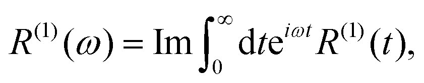


 are the initial condition and the corresponding evolution for the pth sample, respectively.
 after adopting the filtering algorithm.51 Within our choice of parameters and under the high-temperature limit, we found that it is accurate enough for the testing of our NQP model. We set the upper time limit as tmax = 30 fs with a time step of δt = 0.6 fs, which results in Nt = 50 time points.