Valley splitting of monolayer Hf₃C₂O₂ by the spin–orbit coupling effect: first principles calculations using the HSE06 methods

Abstract

Electrons have not only charge and spin degrees of freedom, but also additional valley degrees of freedom. The search for valleytronic materials with large valley splits is important for the development of valleytronics. In this work, we applied first principles computations to calculate 1 L Hf₃C₂O₂ at the level of HSE06. When the spin–orbit coupling (SOC) effect is considered, 1 L Hf₃C₂O₂ is an indirect bandgap semiconductor with a bandgap of 0.952 eV. Meanwhile, valley splitting occurs between the conduction bands Γ and K, with a valley splitting value as high as 98.228 meV. Bader charge analysis was used to determine that Hf–O and Hf–C are ionic bonds. The computed elastic constants and phonon spectra proved that 1 L Hf₃C₂O₂ is mechanically and dynamically stable. In addition, the Berry curvature of 1 L Hf₃C₂O₂ is non-zero. In the work the effect of the electronic properties of 1 L Hf₃C₂O₂ was also calculated with respect to the biaxial strain. The results show that the biaxial strain can well regulate the band gap and valley splitting. Finally, we calculated the effects of hole and electron doping on the band gap and valley splitting of 1 L Hf₃C₂O₂. The results show that the band gap and valley splitting are linearly related to the doping concentration. Our study shows that 1 L Hf₃C₂O₂ is a promising two-dimensional valleytronics material.

---

1. Introduction

The concept of energy valleys has already been mentioned in 3D system materials in 1977.¹ An energy valley refers to the extreme point in an energy band, whether it is the valence band or the conduction band, the extreme point is the energy valley, and these positions are generally near the Fermi level. In k-spaces with special symmetric materials, there are multiple energy degenerate valleys. Under certain external conditions, the simplicity of these energy valleys will be broken, so that the electrons in the energy valleys show dynamic polarization effects. From a theoretical point of view, these energy valleys can be viewed as discrete degrees of freedom, which are used to label information. Similar to electron and spin degrees of freedom, there is potential for coding and information storage functions, providing a theoretical basis for the development of next-generation electronic devices.

Since graphene has been successfully prepared experimentally, the study of 2D valleytronics has attracted a lot of attention.² In addition to charge and spin, the electrons have a new degree of freedom called the valley degree of freedom. It is usually the robust to smooth deformation and scattering of long-wave phonons,³ which are important for practical applications. Therefore, the valley index is very popular as a new information carrier. In order to fully realize the valley index, the ultimate goal is to break the simplicity of the energy bands.⁴

In recent years, there have been many candidate materials for two-dimensional valleytronics. For example, germanene,⁵ transition metal disulfides,⁶ the 2D MA₂Z₄ family^7–10 and 2D transition metal carbides and/or nitrides (MXenes).^11,12 At present, the most popular and the largest number of 2D valleytronics materials are 2D transition metal sulfides, with a chemical formula of MX₂ (M = Cr, Mo, W, etc., and X is the coordination element).^2,12–14 Transition metal carbides and/or nitrides, as the largest known family of 2D materials, have received extensive attention due to their layered structures.

A new family of 2D materials (MXenes) consisting of transition metal carbides and/or nitrides are the most promising materials due to their superb properties.¹⁵ Ti₃C₂T_x was the first MXenes to be discovered and has been in the spotlight as a representative member of the MXenes family.¹² MXenes are typically prepared by selectively etching out element A from the bulk phase MAX, where A is a group IIIA to VIA element. The general formula is M_n+1X_nT_x (M is a transition metal atom, X is a carbon/nitrogen atom, and T_x is a halogen element).¹⁶ Valleytronics in MXene materials have been reported in recent years. For example, Li and He et al. found that a 2D Janus Cr₂COF (∼334 meV) can generate valley polarization.¹⁷ Lu and Liu et al. found that Y₃N₂O₂ (∼21.3 meV) and La₃N₂O₂ (∼100.4 meV) also exhibit valley polarization.¹⁸ Lan et al. found that W₂NSCl (∼83 meV and ∼491 meV) has valley splitting.¹⁹ However, reports related to the valleytronics of MXene materials are still rare.

In this work, the HSE06 method is employed to calculate the first principles of 1 L Hf₃C₂O₂. When SOC is considered, the band gap of 1 L Hf₃C₂O₂ is 0.952 eV. At the same time, the valley splitting occurs between the conduction bands Γ and K, with a valley splitting value of 98.228 meV. In addition, the stability of 1 L Hf₃C₂O₂ is calculated. The results show that 1 L Hf₃C₂O₂ is mechanically and dynamically stable. In this work the Berry curvature of 1 L Hf₃C₂O₂ was calculated and is found to be non-zero. The biaxial strain is an effective method to regulate the electronic properties. Therefore, the influence of the electronic properties of 1 L Hf₃C₂O₂ on the biaxial strain is calculated. The results show that the biaxial strain can well regulate the band gap and valley splitting. Our study shows that 1 L Hf₃C₂O₂ is a promising 2D valleytronics material.

2. Computational methods

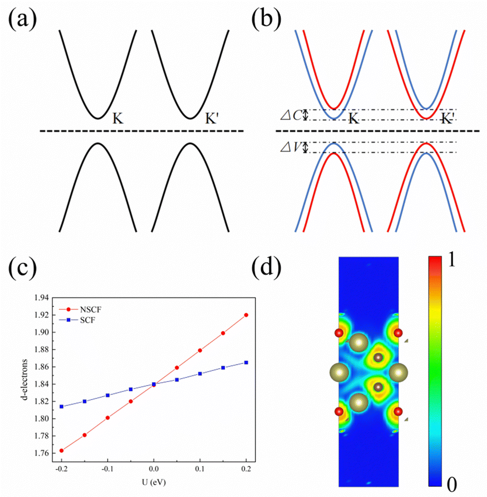
The first-principles computations are used based on the density-functional theory (DFT)²⁰ in the Vienna Ab initio Simulation Package (VASP).^21,22 The projected affixed wave (PAW) method is used to describe the interaction between electrons and ions.^23,24 The Perdew–Burke–Ernzerhof (PBE) functional is used to deal with exchange correlation potential in generalized gradient approximation (GGA).²⁵ The GGA+U²⁶ method is used to correct the strongly correlated d-orbital electrons, where the U value is calculated by the linear response method.²⁷ In this paper, parameters U and J are set in an efficient manner. After calculation, the linear response of Hf₃C₂O₂ is shown in Fig. 2(c), where U_eff = (U − J) = 5.295 eV. Meanwhile, the Heyd–Scuseria–Ernzerhof hybrid functional (HSE06) method is used to calculate the electronic structure.²⁸ The cutoff energy is set to 500 eV. The convergence criterion for the force is 0.01 eV Å⁻¹. The convergence standard of energy is 10⁻⁶ eV. A vacuum layer of 15 Å is provided in the z-direction. A 15 × 15 × 1 Monkhorst–Pack k-point grid was used to sample the 2D Brillouin zone, where Γ is located at the center of the Brillouin zone.²⁹ The DFT-D3 method was used to correct the interlayer van der Waals forces.³⁰ The phonon spectrum is calculated using the PHONOPY code,³¹ taking a grid of k points of 3 × 3 × 1 and using a supercell of 4 × 4 × 1. The SOC effect is also considered to calculate the electronic structure of the material.³² The PYPROCAR code was used to draw spin polarized energy bands.³³ Finally, the Berry curvature of the whole 2D Brillouin zone is calculated using the Vaspberry code.

3. Results and discussion

3.1. Structure and stability

The top and side views of the 1 L Hf₃C₂O₂ crystal structure are shown in Fig. 1(a) and (c). The space group of 1 L Hf₃C₂O₂ is P6/mmm (No. 191). It has a hexagonal honeycomb structure. After optimization, the lattice constant of 1 L Hf₃C₂O₂ is a = b = 3.252 Å. The thickness of the 1 L Hf₃C₂O₂ is 7.645 Å, the bond length of Hf and O atoms is 2.122 Å, the bond length of the uppermost Hf and C atoms is 2.340 Å, and the bond length of the middle layer Hf and C atoms is 2.365 Å. The spatial inversion symmetry of the 1 L Hf₃C₂O₂ crystal structure is broken. The high symmetry points of the Brillouin zone are also shown in Fig. 1(b).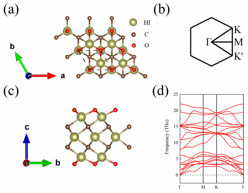

Fig. 1 (a) Top view of the 1 L Hf₃C₂O₂ crystal structure. (b) High symmetry points in the Brillouin zone of 1 L Hf₃C₂O₂. (c) Side view of the 1 L Hf₃C₂O₂ crystal structure. (d) Phonon spectrum of 1 L Hf₃C₂O₂.

Fig. 2 (a) Schematic diagram of energy bands when SOC is not considered. (b) Schematic of energy bands when SOC is considered. (c) Linear response diagram of 1 L Hf₃C₂O₂, with the horizontal coordinates representing the applied effective Coulomb field and the exchange interaction term, and the vertical coordinates representing the number of d-orbital charge occupations of the plus U atom. (d) Plot of the electronic localization function of 1 L Hf₃C₂O₂.

Since the structural stability is important for the applications, in this work, to determine the stability of 1 L Hf₃C₂O₂, we calculated the phonon spectrum and elastic constants. First, in this work the phonon spectrum of the whole Brillouin region along the high symmetric point Γ–M–K–Γ was obtained, as shown in Fig. 1(d). From the phonon spectrum, there is no imaginary frequency in the phonon spectrum of 1 L Hf₃C₂O₂, which indicates that 1 L Hf₃C₂O₂ is dynamically stable. Then, in this work the elastic constants of 1 L Hf₃C₂O₂ are calculated, which are C₁₁ = 331.31 N m⁻¹, C₁₂ = 95.17 N m⁻¹, and C₆₆ = 118.07 N m⁻¹, satisfying the Born criterion:^34,35

C₁₁ > 00, C₁₁ > |C₁₂|

This indicates that 1 L Hf₃C₂O₂ is mechanically stable. Based on the elastic constant, the Young's modulus and Poisson's ratio of Hf₃C₂O₂ are also calculated. The Young's modulus characterizes the softness or hardness of a material;³⁶ commonly graphene has a Young's modulus of 340 N m⁻¹ and MoS₂ has a Young's modulus of 129 N m⁻¹.³⁷ The Young's modulus of 1 L Hf₃C₂O₂ was calculated to be 303.97 N m⁻¹, which indicates that the softness and hardness of 1 L Hf₃C₂O₂ is basically comparable to that of graphene and is tougher than that of MoS₂. Poisson's ratio characterizes the ratio of the transverse dimensional change to the longitudinal dimensional change when the material is strained. Most 2D materials have Poisson's ratios within 0–0.5.³⁸ The Poisson's ratio for 1 L Hf₃C₂O₂ is 0.287, whereas it is 0.25 for MoS₂ and 0.3 for CrSe₂. The results indicate that 1 L Hf₃C₂O₂ has a moderate mechanical response to external loads. Overall, 1 L Hf₃C₂O₂ is mechanically and kinetically stable, which also suggests that 1 L Hf₃C₂O₂ can be synthesized in the experiment.

3.2. Electronic properties and valley splitting

To study the bonding properties of 1 L Hf₃C₂O₂, we used the Bader charge analysis method for charge transfer. The results show that there is a significant charge transfer in 1 L Hf₃C₂O₂. For example, the Hf atom in the middle layer lost 2.04 electrons. The top Hf atom lost 1.52 electrons. The bottom Hf atom lost 1.52 electrons. The C atom in the upper layer gained 1.55 electrons. The lower C atom gained 1.55 electrons. The O atom in the upper layer gained 0.99 electrons. The lower O atom gained 0.99 electrons. In terms of the number of electrons gained and lost, the atoms in 1 L Hf₃C₂O₂ have a large number of electrons gained and lost, and the gain and loss of electrons is more pronounced. This suggests that there is an ionic bond between the Hf atom and the C atom, as well as an ionic bond between the Hf atom and the O atom. In order to determine the bonding properties of 1 L Hf₃C₂O₂, we used the electronic states for analysis, as shown in Fig. 2(d). The electrons are mainly distributed around O and C atoms, with some localized around Hf atoms, suggesting that the Hf–O and Hf–C bonds have ionic properties. This result is consistent with the Bader charge analysis.

To study the electronic properties of 1 L Hf₃C₂O₂, we calculated the energy band structure. Fig. 3(a) and (b) are schematic illustrations of valley splitting. Fig. 2(a) is a schematic diagram of the energy bands that are simple when SOC is not considered. When SOC is considered, a large change in the energy bands occurs and the simplicity is broken, producing valley splitting, as shown in Fig. 2(b). ΔC and ΔV denote the size of the conduction and valence band splits, respectively. Therefore, when SOC is not considered, 1 L Hf₃C₂O₂ is an indirect bandgap semiconductor with a bandgap of 0.979 eV, as shown in Fig. 3(a). The top of the valence band is located at point Γ in the Brillouin zone, while the bottom of the conduction band is located at point M in the Brillouin zone. Since transition metals have very strong SOC, the energy band structure of 1 L Hf₃C₂O₂ changes when SOC is considered, as shown in Fig. 3(b). 1 L Hf₃C₂O₂ remains an indirect bandgap semiconductor. The positions of the valence band tops and conduction band bottoms are the same as when SOC is not considered. When SOC is considered, the biggest change is that the simplicity of the energy band is broken, resulting in valley splitting. The valley splitting value between Γ and K is 98.228 meV. It is higher than the valley splitting values of 50 meV for ZrNCl³⁹ and 63 meV for CrSiGeN₄,⁴⁰ and 70 meV for TiBrI.⁴¹

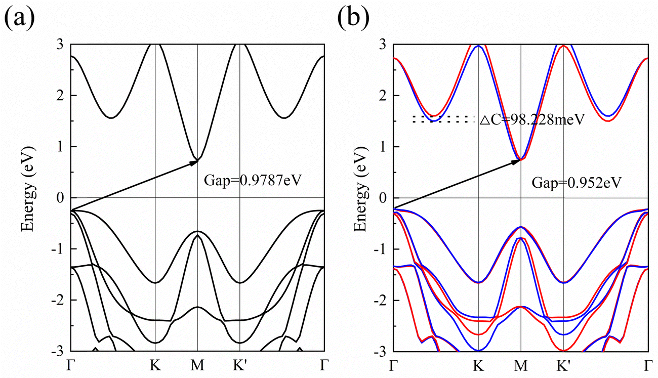Fig. 3 (a) Energy band diagram calculated by the method of HSE06 when SOC is not considered. (b) Energy band diagram calculated by the method of HSE06 when the SOC is considered, where red represents spin up and blue represents spin down.

In this work, we also used the PBE and GGA+U methods for computing the energy bands of 1 L Hf₃C₂O₂, as shown in Fig. 4. Fig. 4(a) and (b) show the energy bands calculated by the PBE method. When SOC is not considered, 1 L Hf₃C₂O₂ is also an indirect bandgap semiconductor with a bandgap of 0.428 eV. The valence band top is similarly located at the Γ point in the Brillouin zone, while the conduction band bottom is also located at the M point in the Brillouin zone.

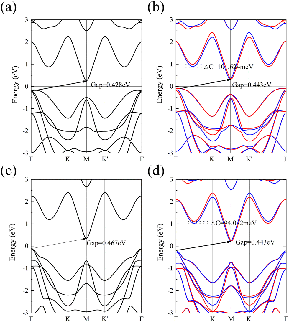Fig. 4 (a) Energy band diagram calculated using the PBE method when SOC is not considered. (b) Energy band diagram calculated using the PBE method when SOC is considered. (c) Energy band diagram calculated using the GGA+U method when SOC is not considered. (b) Energy band diagram calculated using the GGA+U method when SOC is considered. Red represents spin up and blue represents spin down.

When SOC is considered, 1 L Hf₃C₂O₂ remains an indirect bandgap semiconductor with a bandgap of 0.443 eV. The valley splitting was produced between Γ and K, with a valley splitting value of 101.624 meV. Fig. 4(c) and (d) show the energy bands calculated by the GGA+U method. Similarly, when SOC is not considered, 1 L Hf₃C₂O₂ is an indirect bandgap semiconductor with a bandgap of 0.467 eV. The top of the valence band is located at the Γ point in the Brillouin zone, while the bottom of the conduction band is located at the M point in the Brillouin zone. When SOC is considered, 1 L Hf₃C₂O₂ remains an indirect bandgap semiconductor with a bandgap of 0.443 eV. The positions of the top of the valence band and the bottom of the conduction band remain constant. Valley splitting was produced between Γ and K with a valley splitting value of 94.072 meV. Regarding the accuracy of the calculations, the HSE06 method is more accurate than the PBE and GGA+U methods in determining the electronic properties.

In order to study the source of valley splitting in 1 L Hf₃C₂O₂, the local state density and partial state density of 1 L Hf₃C₂O₂ were calculated respectively. As shown in Fig. 5(a), in the localized density of states diagram for 1 L Hf₃C₂O₂ red represents the electron occupation number of the transition metal atom Hf, and green and blue represent the electron occupation numbers of the C and O atoms, respectively. Based on the energy band diagram we know that the valley splitting of 1 L Hf₃C₂O₂ is above the Fermi energy level, so we mainly look at the part of the localized state density above the Fermi energy level. It can be concluded that above the Fermi surface it is mainly occupied by electrons of transition metal Hf atoms. More specifically, we are able to determine that the energy bands above the Fermi surface are mainly occupied by the d orbitals of the transition metal Hf atoms based on the partial state density map of 1 L Hf₃C₂O₂, where yellow, violet, and red represent the number of electrons occupying the d, p, and s orbitals of the transition metal Hf atoms, respectively. In order to determine more clearly the specific form of the contribution of the d-orbitals of Hf atoms to valley splitting, we plotted the projected energy band diagram of the d-orbitals of Hf atoms as shown in Fig. 5(b). Between Γ and K, the valley splitting of the conduction band is mainly contributed by the d_x²–y² orbitals of the Hf atoms. The valley splitting between K′ and Γ is mainly contributed by the d_z² and d_x²–y² and d_xy orbitals of the Hf atom.

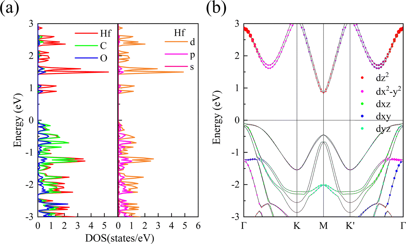Fig. 5 (a) Localized density of states for 1 L Hf₃C₂O₂ and partial wave density of states for the transition metal element Hf. (b) Energy band diagram of the d-orbital projection of 1 L Hf₃C₂O₂. The Fermi energy level is set to 0 eV.

3.3. Berry curvature

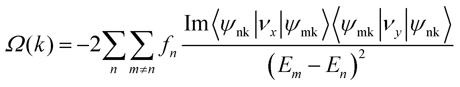
Since 1 L Hf₃C₂O₂ breaks spatial inversion symmetry but is protected by temporal inversion symmetry, 1 L Hf₃C₂O₂ should have Berry curvature with opposite directions but equal values. To confirm this, we calculated the out-of-plane Berry curvature of the conduction band where the 1 L Hf₃C₂O₂ valley splitting is located. The Berry curvature can be written as:⁴²
where f_n denotes the Fermi–Dirac distribution function, ν_x/ν_y denotes the velocity operator of the Bloch function along the direction, and ψ_nk/ψ_mk denotes the wave function with eigenvalues. Due to the breaking of the inversion symmetry of 1 L Hf₃C₂O₂, the carriers in the K/K′ valley of 1 L Hf₃C₂O₂ have a non-zero Berry curvature along the out-of-plane direction. However, under the protection of time reversal symmetry, the Berry curvature satisfies −Ω_n(k) = Ω_n(−k). The Berry curvature of K/K′ is equal in magnitude and opposite in direction, as shown in Fig. 6(a). As we can see from the figure, there are alternating areas of dark blue and dark red at K and K′, and the darker the color, the larger the value.

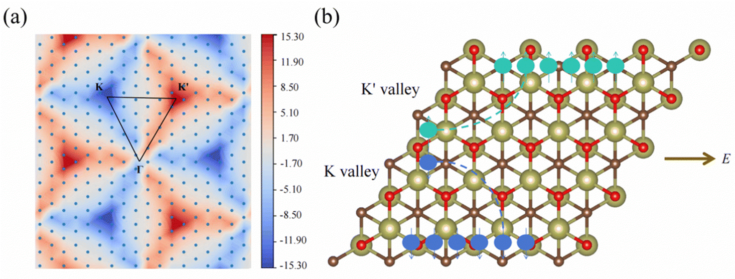Fig. 6 (a) Contour plot of the Berry curvature of 1 L Hf₃C₂O₂ in the whole Brillouin zone. (b) Schematic of the anomalous valley Hall effect in the K/K′ valley, with arrows indicating spin-up and spin-down states and circles indicating holes.

The valley splitting in Hf₃C₂O₂ occurs between Γ–K, not on K/K′. From the band structure, the local maximum between Γ–K is 98.228 meV for valley splitting, while on K/K′, there is a maximum of 208.815 meV. From the graph of Berry curvature, this conclusion can be verified. We can see from the graph of the Berry curvature that on K/K′, the color of the Berry curvature is the darkest, representing the maximum of the Berry curvature, and there is a local value between Γ–K. The Berry curvature corresponds to the band structure.

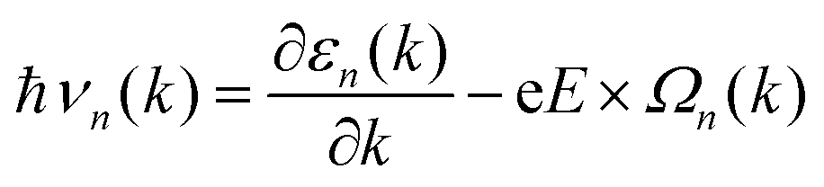
Due to the non-zero Berry curvature of 1 L Hf₃C₂O₂, when an in-plane electric field E is applied, the Bloch electrons exhibit anomalous velocities perpendicular to the electric field:¹⁴

where, the second part of the above formula expresses the meaning of the abnormal velocity proportional to the Berry curvature. In the above section we have calculated the Berry curvature of 1 L Hf₃C₂O₂ and obtained that the K and K′ points in the Brillouin zone have opposite Berry curvatures. Therefore, electrons in the K valley and K′ valley deflect in opposite directions. Electrons in the K valley deflect downwards, while electrons in the K′ valley deflect upwards,⁴³ thus achieving the anomalous Valley Hall effect, as shown in Fig. 6(b).

3.4. Biaxial strain

2D materials can often withstand large lattice strains and their properties can be effectively tuned by strain engineering.⁴⁴ Biaxial strain can be expressed as:
where a₀ refers to the lattice constant of the material when no biaxial strain is applied and a represents the lattice constant after biaxial strain is applied. A negative value of ε indicates a compressive strain on the material and a positive value of ε indicates a tensile strain on the material. Therefore, the present work also calculates the variation patterns of band gap and valley splitting values under biaxial strain. As shown in Fig. 7(a), the band gap first increases and then decreases with strain. The band gap is maximized at 1% applied strain with a maximum value of 0.962 eV. As shown in Fig. 7(b), the valley splitting of the conduction band increases with the increase of strain. When a strain of 4% is applied, the valley splitting value reaches its maximum, which is 104.358 meV. Therefore, the band gap and valley splitting of 1 L Hf₃C₂O₂ are robust. To reflect the evolution trend of its electronic properties, we plotted the band structure of 1 L Hf₃C₂O₂ under strains of −4% to 4%, as shown in Fig. S1 (ESI†).

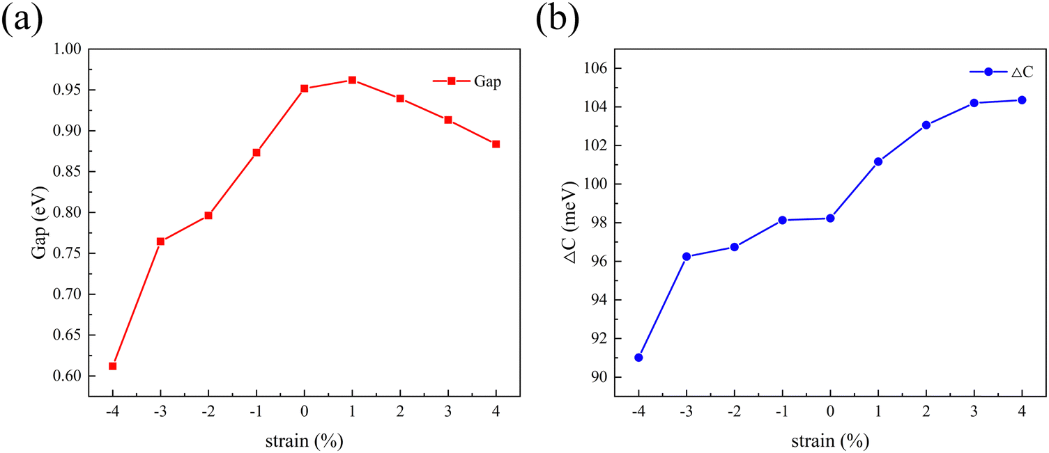Fig. 7 Plots of the variation in (a) band gap and (b) valley splitting values of Hf₃C₂O₂ when biaxial strains from −4% to 4% are applied.

3.5. Doping

To demonstrate the doping effect, the band gaps and valley splitting as a function of the electron and hole doping concentration are investigated. As shown in Fig. 8(a), the band gap increases with increasing hole doping concentration. Instead, the band gap becomes smaller with increasing electron doping concentration. Similarly, the relationship between valley splitting and doping concentration is the same, as shown in Fig. 8(b). The valley splitting increases with more hole doping, while the valley splitting decreases with more electron doping. Therefore, for 1 L Hf₃C₂O₂, hole doping is a feasible way to increase the valley splitting. To reflect the evolution trend of its electronic properties, we plotted the band structure of 1 L Hf₃C₂O₂ with doping concentrations ranging from −0.1 electron per unit cell to 0.1 electron per unit cell in Fig. S2 (ESI†).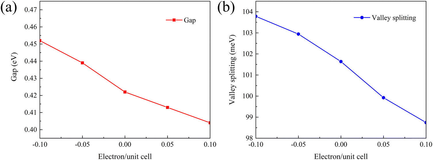

Fig. 8 Curves of (a) band gap and (b) valley splitting of 1 L Hf₃C₂O₂ with doping concentration. 0.00 means neither gain nor loss of electrons, a negative number means loss of electrons (hole doping) and a positive number means gain of electrons (electron doping).

4. Conclusions

In this work, we employed the HSE06 method to determine the properties of 1 L Hf₃C₂O₂. Without considering SOC, 1 L Hf₃C₂O₂ is an indirect bandgap semiconductor. When SOC is taken into account, the bandgap of 1 L Hf₃C₂O₂ decreases. The valley splitting value of 98.228 meV occurs between the Γ and K points in the conduction band. Calculations have verified that 1 L Hf₃C₂O₂ exhibits good mechanical and dynamical stability. Additionally, the Berry curvature of 1 L Hf₃C₂O₂ is non-zero, with equal magnitudes but opposite signs at K and K′. As an effective means of tuning electronic properties, biaxial strain shows good stability for the bandgap and valley splitting of 1 L Hf₃C₂O₂ under such conditions. Both the bandgap and valley splitting values decrease with increasing doping concentration. Our research indicates that 1 L Hf₃C₂O₂ is a promising two-dimensional valleytronics material.

Data availability

All data that support the findings of this study are included within the article (and any ESI† files).

Conflicts of interest

The authors declare that they have no known competing financial interests or personal relationships that could have appeared to influence the work reported in this paper.

Acknowledgements

Supported by the National Natural Science Foundation of China (Grant No. 61704083 and 12104234), the Natural science fund for colleges and universities in Jiangsu Province (Grant No. 21KJD140005), and the Natural Science Foundation of Jiangsu Province (Grant No. BK20210578). The authors gratefully acknowledge the computing time granted by the Shanghai Supercomputer Centre.

References

1. F. J. Ohkawa and Y. Uemura, J. Phys. Soc. Jpn., 1977, 43, 907–916.
2. J. R. Schaibley, H. Yu, G. Clark, P. Rivera, J. S. Ross, K. L. Seyler, W. Yao and X. Xu, Nat. Rev. Mater., 2016, 1, 1–15.
3. Y. Ma, L. Kou, A. Du, B. Huang, Y. Dai and T. Heine, Phys. Rev. B, 2018, 97, 035444.
4. Z. Wang, X. Han and Y. Liang, Phys. Chem. Chem. Phys., 2024, 26, 17148–17154.
5. G. Liu, S. Liu, B. Xu, C. Ouyang and H. Song, J. Appl. Phys., 2015, 118, 124303.
6. C. Tan and H. Zhang, Chem. Soc. Rev., 2015, 44, 2713–2731.
7. A. Bafekry, C. Stampfl, M. Naseri, M. M. Fadlallah, M. Faraji, M. Ghergherehchi, D. Gogova and S. Feghhi, J. Appl. Phys., 2021, 129, 155103.
8. J.-S. Yang, L. Zhao, L. Shi-Qi, H. Liu, L. Wang, M. Chen, J. Gao and J. Zhao, Nanoscale, 2021, 13, 5479–5488.
9. J. Yuan, Q. Wei, M. Sun, X. Yan, Y. Cai, L. Shen and U. Schwingenschlögl, Phys. Rev. B, 2022, 105, 195151.
10. P. Li, X. Yang, Q.-S. Jiang, Y.-Z. Wu and W. Xun, Phys. Rev. Mater., 2023, 7, 064002.
11. C. E. Shuck and Y. Gogotsi, Chem. Eng. J., 2020, 401, 125786.
12. S. Venkateshalu, M. Shariq, B. Kim, M. Patel, K. S. Mahabari, S.-I. Choi, N. K. Chaudhari, A. N. Grace and K. Lee, J. Mater. Chem. A, 2023, 11, 13107–13132.
13. G.-B. Liu, D. Xiao, Y. Yao, X. Xu and W. Yao, Chem. Soc. Rev., 2015, 44, 2643–2663.
14. X. Xu, W. Yao, D. Xiao and T. F. Heinz, Nat. Phys., 2014, 10, 343–350.
15. Y. Gogotsi and B. Anasori, Journal, 2019, 13, 8491–8494.
16. M. Naguib, V. N. Mochalin, M. W. Barsoum and Y. Gogotsi, Adv. Mater., 2014, 26, 992–1005.
17. S. Li, J. He, L. Grajciar and P. Nachtigall, J. Mater. Chem. C, 2021, 9, 11132–11141.
18. J. Lu, R. Liu, F. Yue, X. Zhao, G. Hu, X. Yuan and J. Ren, J. Phys. Chem. Lett., 2022, 14, 132–138.
19. M. Lan, S. Wang, X. Liu, S. Ma, S. Qiao, Y. Li, H. Wu, F. Li and Y. Pu, Phys. Chem. Chem. Phys., 2024, 26, 8945–8951.
20. W. Kohn and L. J. Sham, Phys. Rev., 1965, 140, A1133–A1138.
21. G. Kresse and J. Hafner, Phys. Rev. B: Condens. Matter Mater. Phys., 1993, 48, 13115.
22. G. Kresse and J. Furthmüller, Comput. Mater. Sci., 1996, 6, 15–50.
23. G. Kresse and J. Furthmüller, Phys. Rev. B: Condens. Matter Mater. Phys., 1996, 54, 11169–11186.
24. V. Milman, B. Winkler, J. White, C. Pickard, M. Payne, E. Akhmatskaya and R. Nobes, Int. J. Quantum Chem., 2000, 77, 895–910.
25. Y. Zhang and W. Yang, Phys. Rev. Lett., 1998, 80, 890.
26. S. L. Dudarev, G. A. Botton, S. Y. Savrasov, C. Humphreys and A. P. Sutton, Phys. Rev. B: Condens. Matter Mater. Phys., 1998, 57, 1505.
27. M. Cococcioni and S. De Gironcoli, Phys. Rev. B: Condens. Matter Mater. Phys., 2005, 71, 035105.
28. J. Heyd and G. E. Scuseria, J. Chem. Phys., 2004, 121, 1187–1192.
29. H. J. Monkhorst and J. D. Pack, Phys. Rev. B: Solid State, 1976, 13, 5188.
30. S. Grimme, J. Antony, S. Ehrlich and H. Krieg, J. Chem. Phys., 2010, 132, 15.
31. A. Togo, F. Oba and I. Tanaka, Phys. Rev. B: Condens. Matter Mater. Phys., 2008, 78, 134106.
32. M. Blume and R. Watson, Proceedings of the Royal Society of London. Series A. Mathematical Physical Sciences, 1963, 271, 565–578.
33. U. Herath, P. Tavadze, X. He, E. Bousquet, S. Singh, F. Muñoz and A. H. Romero, Comput. Phys. Commun., 2020, 251, 107080.
34. Y. Wang, M. Qiao, Y. Li and Z. Chen, Nanoscale Horiz., 2018, 3, 327–334.
35. R. Peng, Y. Ma, B. Huang and Y. Dai, J. Mater. Chem. A, 2019, 7, 603–610.
36. Y. Li, X. Xu, M. Lan, S. Wang, T. Huang, H. Wu, F. Li and Y. Pu, Phys. Chem. Chem. Phys., 2022, 24, 25962–25968.
37. S. Singh, C. Espejo and A. H. Romero, Phys. Rev. B, 2018, 98, 155309.
38. D. Çakır, F. M. Peeters and C. Sevik, Appl. Phys. Lett., 2014, 104, 203110.
39. P. Zhao, Y. Liang, Y. Ma and T. Frauenheim, Phys. Rev. B, 2023, 107, 035416.
40. Y. Li, M. Lan, S. Wang, T. Huang, Y. Chen, H. Wu, F. Li and Y. Pu, Phys. Chem. Chem. Phys., 2023, 25, 15676–15682.
41. Y. Wang, W. Wei, H. Wang, N. Mao, F. Li, B. Huang and Y. Dai, J. Phys. Chem. Lett., 2019, 10, 7426–7432.
42. W. Yao, D. Xiao and Q. Niu, Phys. Rev. B: Condens. Matter Mater. Phys., 2008, 77, 235406.
43. W. Tong, S. Gong, X. Wan and C. Duan, Nat. Commun., 2016, 7, 13612.
44. S. Li, W. Wu, X. Feng, S. Guan, W. Feng, Y. Yao and S. A. Yang, Phys. Rev. B, 2020, 102, 235435.

---

Footnotes

† Electronic supplementary information (ESI) available. See DOI: https://doi.org/10.1039/d4cp04003a

‡ Shiqian Qiao and Yang Zhang contributed equally to this manuscript.

---