SANE: strategic autonomous non-smooth exploration for multiple optima discovery in multi-modal and non-differentiable black-box functions†
Received
19th September 2024
, Accepted 8th February 2025
First published on 18th February 2025
Abstract
Both computational and experimental material discovery bring forth the challenge of exploring multidimensional and multimodal parameter spaces, such as phase diagrams of Hamiltonians with multiple interactions, composition spaces of combinatorial libraries, material structure image spaces, and molecular embedding spaces. Often these systems are black-boxes and time-consuming to evaluate, which resulted in strong interest towards active learning methods such as Bayesian optimization (BO). However, these systems are often noisy which make the black box function severely multi-modal and non-differentiable, where a vanilla BO can get overly focused near a single or faux optimum, deviating from the broader goal of scientific discovery. To address these limitations, here we developed Strategic Autonomous Non-Smooth Exploration (SANE) to facilitate an intelligent Bayesian optimized navigation with a proposed cost-driven probabilistic acquisition function to find multiple global and local optimal regions, avoiding the tendency to becoming trapped in a single optimum. To distinguish between a true and false optimal region due to noisy experimental measurements, a human (domain) knowledge driven dynamic surrogate gate is integrated with SANE. We implemented the gate-SANE into pre-acquired piezoresponse spectroscopy data of a ferroelectric combinatorial library with high noise levels in specific regions, and piezoresponse force microscopy (PFM) hyperspectral data. SANE demonstrated better performance than classical BO to facilitate the exploration of multiple optimal regions and thereby prioritized learning with higher coverage of scientific values in autonomous experiments. Our work showcases the potential application of this method to real-world experiments, where such combined strategic and human intervening approaches can be critical to unlocking new discoveries in autonomous research.
1 Introduction
Recent advancement of automated and autonomous experiments has been transforming the landscape of scientific research.1–5 By integrating experiment automation with machine learning-enabled data analysis and decision-making processes, researchers can now conduct experiments at an unprecedented pace, accelerating the discovery of new materials and the process of characterizing and understanding complex materials systems.
Bayesian Optimization (BO)6–8 is an active learning method which aims to autonomously explore the parameter space and continually learns the unknown ground truth and its global optimal region, where the ground truth function can be either a black-box or expensive to evaluate, or both. Given a few evaluated training samples, the expensive unknown function is replaced by a cheaper surrogate model (e.g. Gaussian process),9–11 and the surrogate model continues to learn the human defined region of interests with adaptive selection (e.g. acquisition function)12–15 of locations for future expensive evaluations. BO is more popular than other design of experiment methods (e.g. random sampling, Latin hypercube sampling, etc.) as it is designed to converge to the optimality with minimal expensive evaluations. Thus, BO has attracted special attention in the materials science domain where accelerated BO driven autonomous discovery has been particularly impactful, enabling efficient identification of optimal conditions for particular material properties without human intervention, such as bandgap optimization,16 small-molecule emitter discovery, maximizing carbon nanotube growth rates,17 and so on. This type of autonomous workflow with BO has been widely used in recent studies to adaptively explore expensive control parameter spaces of physical/simulation models18–23 and experiments,24 material structure–property relationship discovery25 and to develop autonomous platforms towards accelerating chemical26,27 and material design.28–30 Recently, interactive BO frameworks through minor human intervention (human in the loop) proved to have better material processing31 and microscope experimental steering.32–37 A number of excellent reviews on BO are available,6,38 and it is now implemented in a broad range of Python libraries including BOtorch (Pytorch)39 and Gpax (Jax).40
However, the pursuit of optimal conditions, while valuable for application-focused materials development, may not always align with the broader goals of scientific discovery. In the context of scientific and knowledge discovery, understanding the relationships between the vast parameter space and resulting material properties is crucial. The challenge arises when the experimental process becomes overly focused on finding a singular “optimal” condition. This focus can limit the exploration of sub-optimal or diverse conditions that can offer deeper insights into the material's behavior, ultimately advancing our understanding of the underlying principles governing material properties. Moreover, real-world experiments are often subject to noise and other uncertainties, which can lead to “fake” optima—conditions that appear to be optimal due to experimental error or noise but do not represent the true optima. Also, due to such noise, the overall parameter space becomes very non-smooth. Here, we define non-smooth as (1) multi-modal functions which have multiple local and global optimal and (2) non-differentiable functions. So, in this context, a non-differentiable function is a subset of the non-smooth function category. Therefore, the search space becomes much harder to explore, learn the parameter space and locate optimal conditions. In the theory of optimization, numerical methods generally struggle with highly non-smooth functions41 and BO is not an exception due to the surrogate model priors over the belief of a smooth function. It is evident to say that it is even harder to solve a black-box non-smooth function. One can, however, project to a smoother function from such non-smooth functions with the help of either domain knowledge8 or by fitting a cluster of GPs which learn each localized smooth function.42 However, it is a challenging task to always possess appropriate domain knowledge for such projections, or know the number of clusters or region of non-smoothness a priori. Previously BO had been applied to optimize on discrete graph-structured search spaces, by projecting to a graph similarity distance based continuous space via a special kernel function.43 However, a similar correlation cannot be derived always from the noisy experimental data, particularly when the sources of such experimental noises are random. Also, in the case of structure–property learning, the exploration needs to be done over the raw non-smooth function space rather than a projected space to avoid losing critical insights. Thus, when exploring over a non-smooth function due to noisy experiments, when the decision-making process is based on these potentially misleading optimal conditions, there is a risk of missing out on critical information that lies in other sub or near optimal regions. As a result, the classical BO methods may inadvertently limit the scope of exploration in autonomous experimentation.
To address these limitations, we have developed a BO driven Strategic Autonomous Non-Smooth Exploration (SANE) workflow that is designed to navigate and mitigate the challenges posed by noisy experimental data and the tendency to become trapped in local optima. Our SANE framework emphasizes the exploration of a broader range of conditions, including sub-optimal and diverse points within the parameter space. This approach ensures a more comprehensive understanding of the material system being studied, enabling the discovery of new insights and correlations that may otherwise be overlooked. We implemented this SANE approach in two distinct experimental datasets: (1) a piezoresponse spectroscopy hysteresis loop dataset across composition spread of Sm-doped BiFeO3 with high noise levels in specific regions, and (2) a grid piezoresponse spectroscopy hyperspectral dataset over various domain structures of a PbTiO3 thin film. These two datasets have been explored in our previous studies,44–46 indicating that they are good model experimental datasets to demonstrate the application of newly developed ML approaches. In both cases, SANE demonstrated its ability to avoid becoming stuck in noisy regions or singular optima and facilitated the exploration of multiple optimal and sub-optimal conditions. This not only improved the robustness of the optimization process but also provided a more complete picture of the parameter space.
We further enhance our SANE method by adapting a recently developed gated active learning approach46 that allows for the incorporation of human expertise and domain knowledge into the autonomous experimentation process. This hybrid approach leverages the strengths of both autonomous systems and human intuition, allowing for more targeted and effective exploration. By guiding the optimization process with human input constraints, we can prioritize the parameter space that has higher scientific value, thereby improving the overall performance and outcomes of autonomous experiments. Our work showcases the potential of this method through its application to noisy experiments, demonstrating its efficacy in avoiding local optima and uncovering a richer understanding of the material systems under study. As the field of materials science continues to evolve, the development and adoption of such strategic approaches will be critical in unlocking new discoveries and pushing the boundaries of what is possible in autonomous research. Previously Eriksson et al.47 designed a TurBO to identify multiple global and local optima using several local searches with a trust region method. While the general problem domain overlaps with our method, however, there are some major differences in the type of problem these methods will be better suited to. Unlike in TurBO, our method is designed to search over noisy experimental space which generates both true and false optima, no prior knowledge of the number of true local and global optimal regions, and the significance of exploiting a local region can be higher than exploiting a global region based on domain experts’ intended goals.
2 Results and discussion
2.1. SANE framework
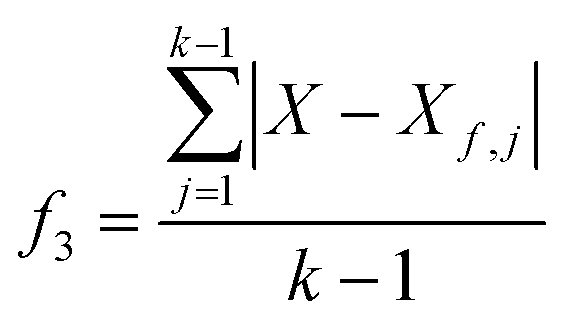
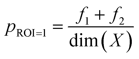
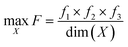
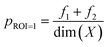
Fig. 1 provides the overall architecture of the proposed SANE workflow with human-intervened dynamic constrained gate, developed over the naïve BO workflow. Unlike in traditional BO, where the acquisition function assumes uniform cost during exploration over the search space, SANE performs a goal orientation exploration with a non-uniform cost of the search space. Cost acquired BO has been developed earlier,48–50 however, the cost function is formulated based on the invariable cost of the experiments over the search space. In this case, we formulate the cost function based on the strategies of (1) discovering a potential global or local region of interest, (2) guiding the exploration centered on new regions of interest and (3) guiding the exploration centered on the previously found region of interests. SANE is initialized as BO where we set the total number of iterations as N. N can be defined as the total cost based on a reasonable time the autonomous experimentation can be performed. As the iteration i progresses, after every n ≪ N iteration, we have a check for discovering a new region of interest. If a solution superior to the current focused solution is found within the samples explored between the current check and previous check, a current or potential global region of interest is found else we perform an optimization routine to find a local optimum sampled after the current focused sample, and then a probabilistic check to determine if the local optimum belongs to a potential region of interest. This optimization scheme is formulated as per eqn (1)–(5). Once the local optimum is found, the binary check of belonging to a region of interest (1 − Yes, 0 − No) is governed by the sampling from logistic distribution with probability, pROI=1 and as pROI=0 respectively, per eqn (6). Let's assume, at iteration i, we have already determined k focused locations. Here, f1 is defined as the absolute distance in the normalized parameter space between the current focused location Xf,k and the location sampled after Xf,k. f2 is defined as the ratio between the output of the location sampled after Xf,k and the output yf,k at Xf,k. Here, f3 is defined as the mean of the absolute distance in the normalized parameter space between each of the previously focused location Xf, and the location sampled after Xf,. As a strategic approach to discover the new region of interest, we would prefer to choose the sample with the farthest distance from all the current and previously focused locations, and closest to the output of the currently focused location. Thus, as per the optimization (maximization) routine, the higher values of the combined product of f1, f2, f3 are chosen. Though it is not always that this best solution belongs to another region of interest, the strategic approach does mean that the likelihood increases with higher values of f1, f2. Therefore, we make a probabilistic decision whether to navigate to the new focused location via sampling from the logistic distribution with probability of mean value of f1, f2. With higher probability, we are likely to add and navigate towards the new focused location (Xf,k+1) and with lower probability, we are likely to consider the current focused location (Xf,k+1 = Xf,k) for the upcoming navigation governed by the strategic cost function.| |  | (3) |
| |  | (4) |
| | | X ∈ {Xarg(Xf,k), …, Xi} ⊆ Di | (5) |
| |  | (6) |
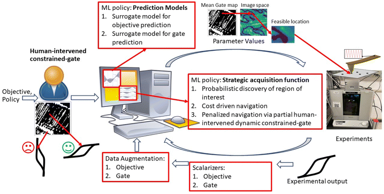 |
| | Fig. 1 Workflow of Strategic Autonomous Non-Smooth Exploration (SANE) with a partial human-intervened dynamic constrained gate. Here, the SANE workflow is shown over AFM experiments but can be implemented in any material characterization technique or any microscopy measurement. Here, the research contribution is the development of the ML policy for a strategic acquisition function, which is subcategorized into (a) probabilistic discovery of region of interest, (b) cost-driven navigation and (c) penalized navigation to explore on feasible search space only, as defined from a partial human-intervened dynamic gate. Here the subject matter expert assesses the quality of the experimental result (e.g. spectral structure) at the initialization of the SANE, and an initial estimated gate map is defined. Then, the estimated gate map is updated with strategic BO driven autonomously sampled new data, without any human intervention. | |
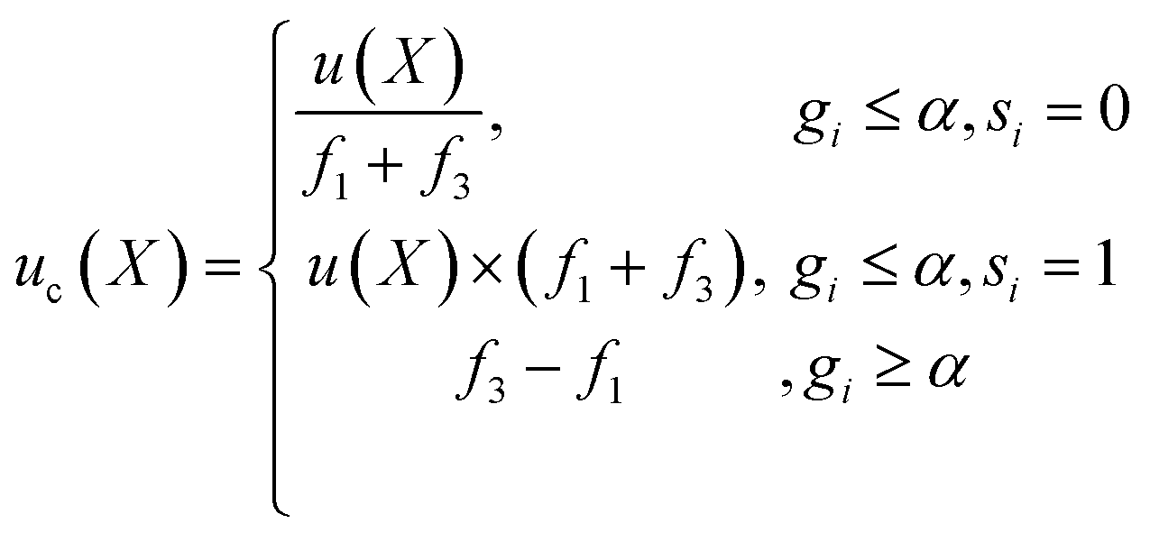
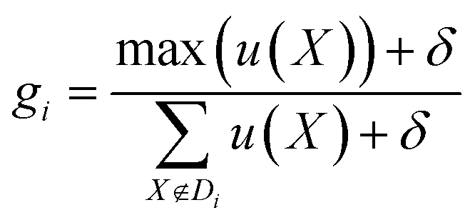
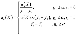
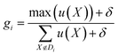
Next, we define the navigation strategy considering all the focused locations. In SANE, strategic exploration is defined as the likelihood of discovering a new region of interest while avoiding becoming trapped over the discovered regions of interest. However strategic exploitation is defined as the likelihood of unearthing critical information over all the discovered regions of interest (optimal and suboptimal points), without only focusing on the singular optimal region. This navigation is governed by a strategic cost function and thus depending on the current state (say iteration i), the cost function puts variable weightage of performing exploration or exploitation. The strategic cost-based acquisition function can be described step by step as follows. Given the mean and variance of the unexplored data from the prediction model as fitted from the explored data, the standard acquisition values of all the unexplored locations are calculated as u(X), X ∉ Di. Here, we can follow any standard acquisition functions in BO such as Probability of Improvement (POI), Expected Improvement (EI) or Upper or Lower Confidence bound (UCB/LCB). Then, the cost driven acquisition function uc(X) can be either exploitative in preference to choose the next sample for function evaluations with the closest distance from the current and previously focused locations, or explorative to prefer to choose the same with the farthest from the current and previously focused locations. It is to be noted that the designed exploration strategy differs from the exploration with considering the model uncertainty only. These would be similar if the problem is smooth where the model uncertainty also monotonically increases with region far away from explorations. However, the case is not the same when the function is very non-smooth.37 Thus, the scope of the paper is not to fully rely on GP based predictions (which assume on prior smooth function) but derive a cost function to heuristically explore. The acquisition function can be mathematically formulated as per eqn (8), assuming at iteration i and k focused locations. Here, s is a switching parameter trajectory with iterative binary choices between strategic exploitation and exploration. s can be pre-defined from the domain expert preference of navigation in the parameter search space. Additionally, to avoid any navigation instability arising due to negligible standard acquisition values almost over the entire search space, we perform the cost driven acquisition function with fully localized search when g ≥ α. δ = 10−5 is a very small value for numerical stability and α is a user defined value between 0 and 1, recommended to be anything α ≥ 0.75. This navigation instability can arise when the standard acquisition function provides false values of negligible information gain in exploring in almost any location during the phase of near optimal learning. However, in a real scenario, this is often not true due to the complex and noisy parameter space and more search is needed and potential better insights can be learned. For strategizing a fully localized search, we would prefer to exploit the current focused locations and avoid exploring again to previously focused locations. This is because such scenarios occur mostly at near optimal learning, where most of the previously focused locations are already exploited and therefore to save cost, we put weight on the local exploration and exploitation only rather than global exploration and exploitation. Thus, we choose the next best sample which has the minimum distance to the current focused locations and maximum distance to the previously focused locations.
| |  | (8) |
| |  | (9) |
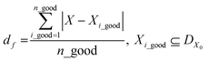
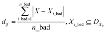
Finally, the SANE workflow is further enhanced with a human assessed constrained gate, to avoid exploring and exploiting “fake” regions of interest due to noisy measurements, thereby avoiding gathering false insights. It is to be noted that the distinction between the strategy of earlier mentioned probabilistic finding of region of interest and the human assessed gate is that the constrained gate narrows down the feasible search space, and within the search space SANE aims to discover the region of interest with the probabilistic approach. In other words, without the gate, SANE can guide to focus on a “fake” region of interest with high probability. Without the region of interest finding strategy, the gate itself will only separate the feasible space but not the discovery of the multiple optimal and suboptimal points (hills in the case of maximization). Previously, human in the loop based autonomous exploration workflows have been developed which proved to have better performance and alignment with the expectation of the experimentalists, than a purely data driven active learning method.32,34–37,51,52 To avoid the increment of the exploration cost (time) in SANE, we include the human assessment during the initialization only where the quality of the initial samples can be accessed (good or bad) via visualization from domain experts. To transform the assessment into a quantitative metric, we compute the mean distance df between selected locations and all feasible assessed locations Xi_good, and mean distance dif between a selected location and all infeasible assessed locations Xi_bad respectively. It is to be noted that Xi_good and Xi_bad combine the initial sampled locations DX0. Then we compute the constraint function as per eqn (10), where a positive value indicates feasibility and a negative value indicates infeasibility.
| | | c ≥ 0 = >dif − df ≥ 0 | (10) |
| |  | (11) |
| |  | (12) |
| | | DX0 = {Xi_good, Xi_bad} | (13) |
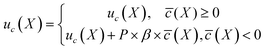
After the initialization as the iteration i progresses, the new samples are not assessed as this would increase the cost of the SANE workflow. Indeed, if the human provides assessment of new experimental data at every iteration, the constraint learning would be better but that will completely increase the cost significantly. Thus, such a trade-off is required. In other words, it is not an appropriate approach for the experimentalist to assess the quality of every SANE navigated sample, as this will completely diminish the purpose of an autonomous workflow. The goal for any human or domain intervened autonomous system would be at the level of minimal intervention with maximum improvement. Thus, the human intervention in the gated-SANE is limited to initialization. During the BO process, for any new samples we have computed the average distance from the bad samples and the good samples which were only initially assessed as Xi_good, Xi_bad ⊆ DX0 where DX0 contains only the initial samples assessed. So, during the BO, we are approximating the feasibility of the new samples based on initial human assessments to balance the acceleration as well, as human assessment at every iteration of constraint validation will decelerate the entire process. However, if more frequent human interaction is required in other application cases, the workflow can be simply adapted for it. Also, in this paper, we have assumed that the human operator is indeed a domain expert. Although the assessment can vary between two domain experts, we have seen that the assessment from non-domain experts (purely random assessment) or attacking users (negative assessment) can derail from the appropriate knowledge.32 However, SANE is entirely not dependent on human intervention. The human intervention in SANE first reduces the parameter space to focus on feasible regions, where then the hybrid acquisition function aims to maximize the feasible global and local regions of interest over exploring non-smooth functions at minimal cost compared to traditional BO. Once the initial assessment is done, an initialized assessed gate constraint datum c is fitted to a surrogate model Δc, and after training, the mean estimation ![[c with combining macron]](https://www.rsc.org/images/entities/i_char_0063_0304.gif) is calculated for all the locations in the parameter space to define the mean estimated gate constraint map. With newly explored locations, the training data are augmented, the gate-surrogate model Δc is retrained, and the mean estimated gate constraint map is updated. Then, the gate constraint is linked to the strategic acquisition function with a penalty factor P as per eqn (14). β is the order of magnitude (ceiling factor) of the maximum value of uc(X), to avoid the imbalance order of magnitude between uc(X) and (X).
is calculated for all the locations in the parameter space to define the mean estimated gate constraint map. With newly explored locations, the training data are augmented, the gate-surrogate model Δc is retrained, and the mean estimated gate constraint map is updated. Then, the gate constraint is linked to the strategic acquisition function with a penalty factor P as per eqn (14). β is the order of magnitude (ceiling factor) of the maximum value of uc(X), to avoid the imbalance order of magnitude between uc(X) and (X).
| |  | (14) |
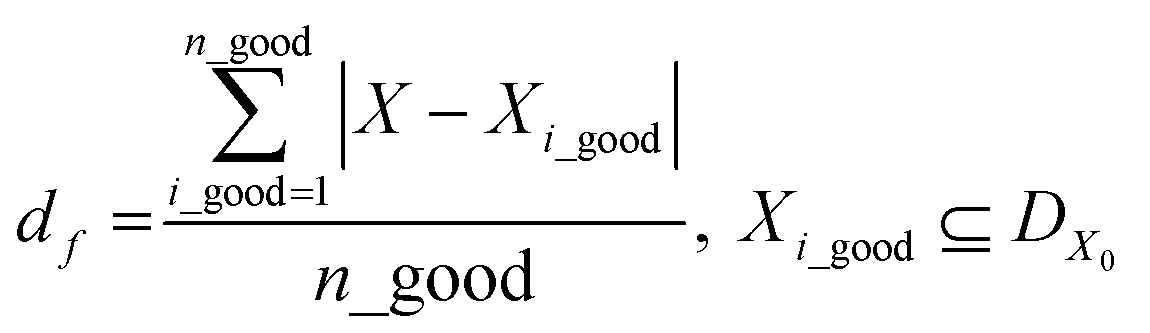
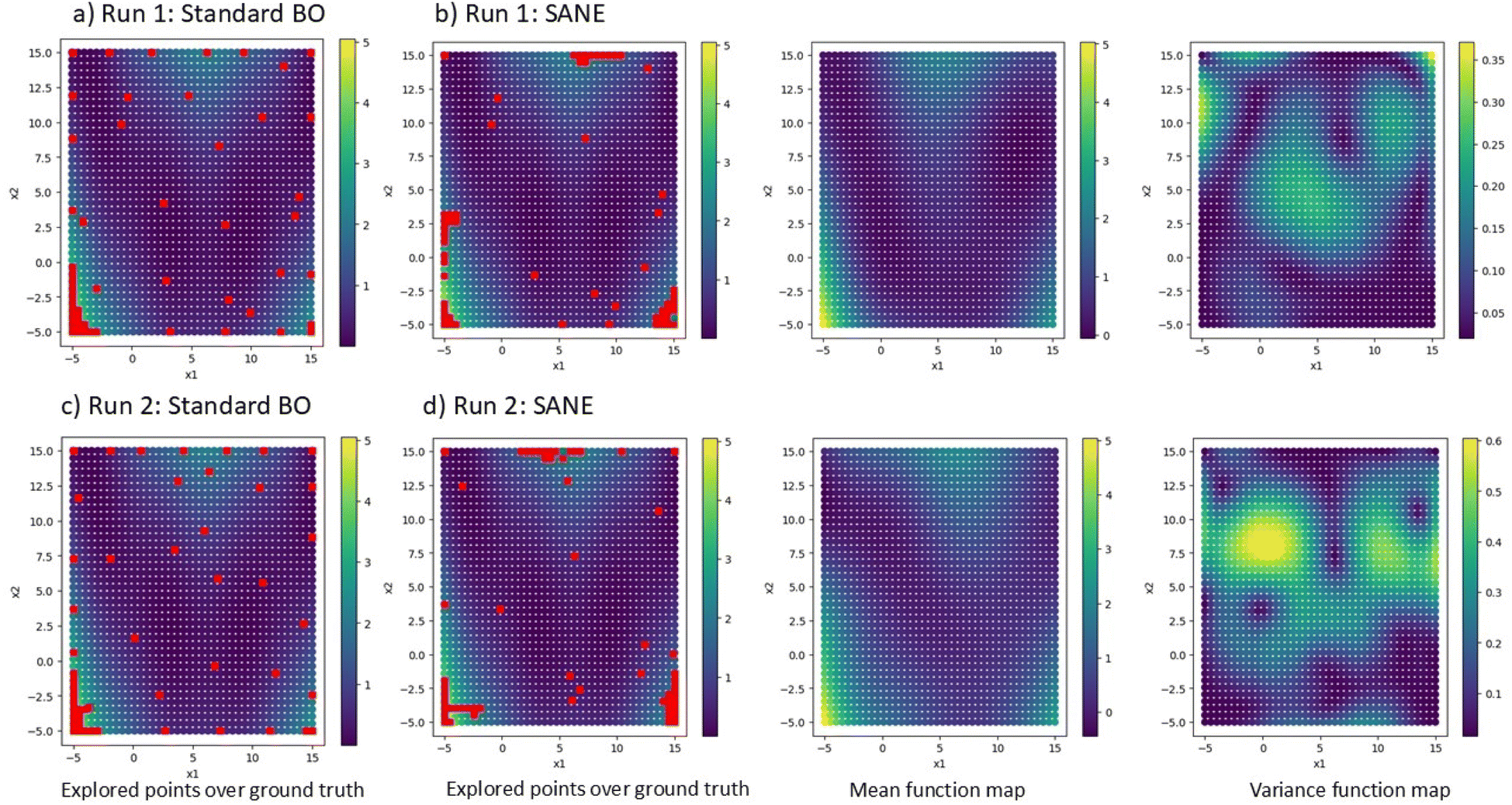
To validate the SANE workflow, we attempt to implement it over a synthetic 2D search space. In this paper, we validated SANE performance based on (1) if SANE has found more regions of interest than BO for a given number of iterations, (2) for a given local region of interest, how many samples have been used to exploit and (3) how many samples have been used in exploring the infeasible region. The 2D test function is the multimodal Branin function,53 containing one global optimum and two local optima. The formulation of the function is provided in the ESI.† The prediction model for data ΔD is considered as a Gaussian process (GP) regression model with Radial Basis kernel function (RBF), and the standard acquisition function u(X) is considered as the Expected Improvement (EI). The detailed formulation of the GP model and EI acquisition function is provided in the ESI.† Here, the switching parameter trajectory is set as si = 0, i < 25 and si = 1, 25 < i ≤ 50. Here, the total number of iterations N = 50. Throughout the paper we consider checking for a new region of interest after every n = 5 iterations. However, the interval number n is set as user input and can be arbitrarily changed as per the user’s choice based on the knowledge of the multi-modal structure of space and how aggressively the user wants to search for a new region of interest. Notably, an arbitrary threshold can also be used to generalize the process along with user choice input, however, a more detailed analysis is required to enable this, which will be updated in the near future. It is evident to say that, since these are non-physical synthetic data, no human-intervened constraint is relevant and therefore we ignore the gate implementation in this example. Fig. 2 shows the overview of the strategic navigation from SANE, to discover and exploit the global and local regions of interest. Fig. 3 shows the comparison of the exploration between the proposed SANE and standard BO, with two initializations. The initial samples for Run 1 are similar to those in Fig. 2a where the initial samples are far away from all the regions of interest. Compared with BO (Fig. 3a), we can clearly see that SANE (Fig. 3b) provides better exploration with high volume of exploitation in all the regions of interest, and better-balanced exploitation among those regions of interest. Contrastingly, BO only focused on exploiting the global region of interest and explored many uninteresting locations rather than exploiting local regions. We see that the estimated function map has a good agreement with the ground truth as well, which again signifies the redundant sampling of BO and better navigation strategy of SANE. In other words, unlike in standard BO, SANE spends more time on finding insights in good regions, while it still performs a good agreement with the overall ground truth. We see similar interpretations with the second initialization, where at least one of the initial samples is within each of the regions of interest (refer to Fig.S1 in the ESI†). Here also the standard BO did not exploit in the local region (Fig. 3c) whereas SANE did (Fig. 3d). To quantify the SANE performance, here we can see that for both cases, SANE exploits 3 out of 3 regions of interest (high function value) while BO exploits only 1. Also, BO explores with an average of 39/60 samples in the true region of interest while SANE explores with an average of 48/60 samples in the true region of interest.
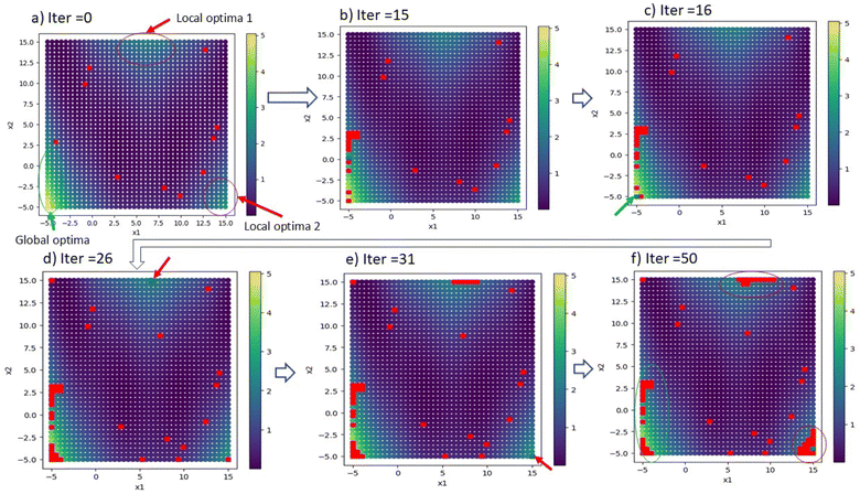 |
| | Fig. 2 Overview of navigation of Strategic Autonomous Non-Smooth Exploration (SANE) on a synthetic 2D search space. Here, the ground truth has one global optimum and 2 local minima. (a) The state of initialization with 10 starting samples randomly selected (denoted by red dots). (b) After 15 iterations, we find the global optimal region and therefore (c) shows the discovery of the global optimal point (denoted by the green dot). (d) The exploitation of the global region of interest and discovery of the first local region of interest (denoted by the green dot) following the probabilistic approach as per eqn (1)–(7). (e) The exploitation of the first local region of interest and discovery of the second local region of interest (denoted by the green dot). (f) The final strategic explored map at iteration 50 with exploitation of both the global and local regions of interest. | |
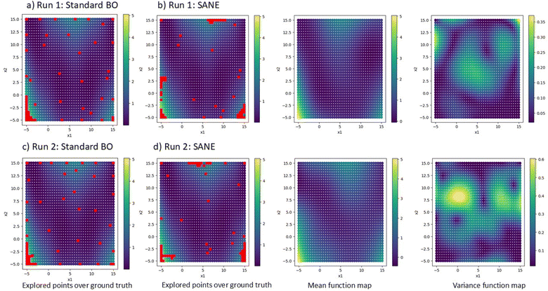 |
| | Fig. 3 Comparison of exploration between BO and SANE on a synthetic 2D search space at two different random initializations. Figures (a) and (c) shows the exploration of BO while figures (b) and (d) shows the exploration of SANE. In figures (b) and (d), the left figures are the explored samples over ground truth, the middle figures are the GP predicted mean and the right figures are the GP uncertainty. | |
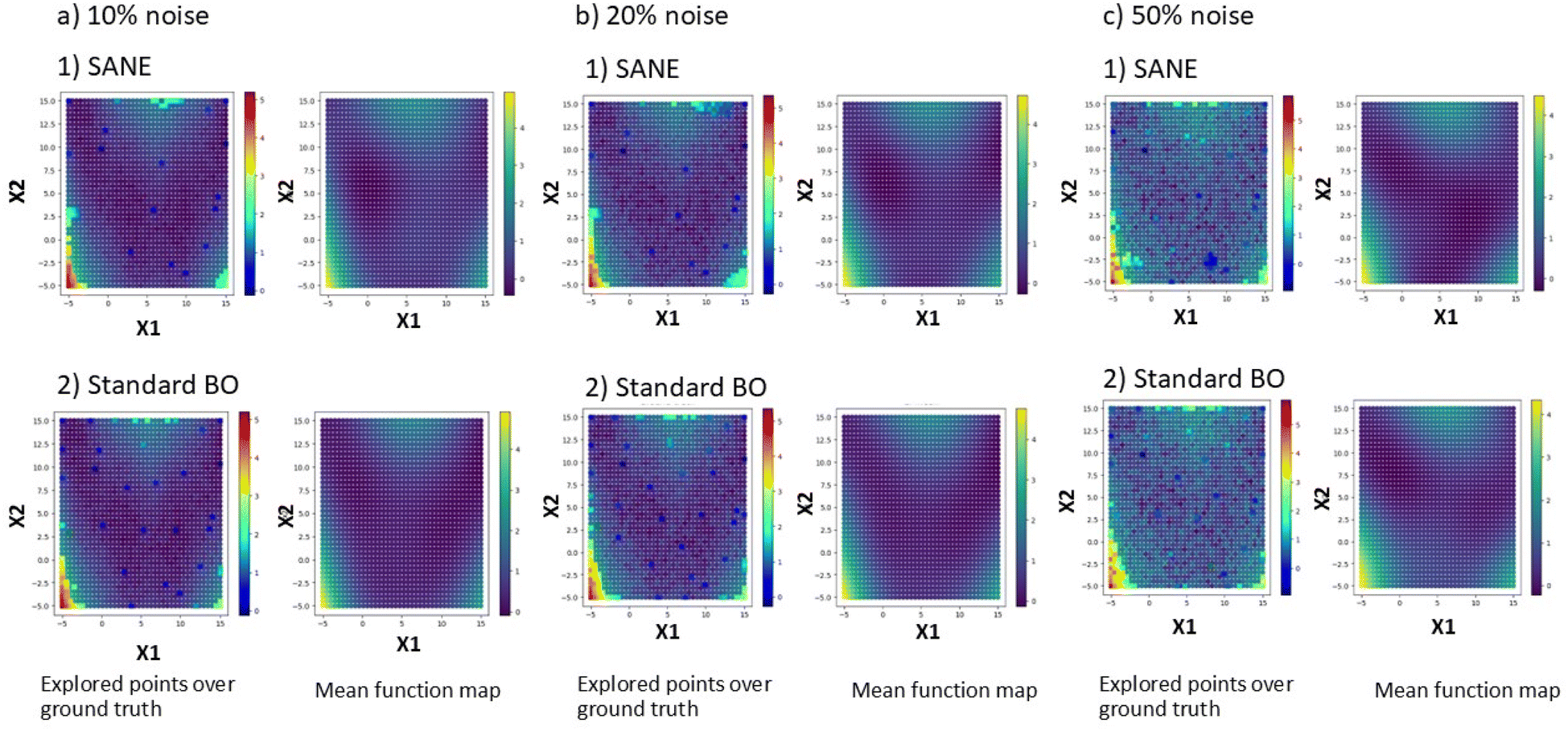
Additionally, we test the SANE by adding different levels of random noise from normal distribution into the ground truth. Fig. 4 shows the comparison of performance between SANE and standard BO. We can see that at low to medium levels of noise (scale ranges at 10% and 20% of ground truth), SANE outperforms standard BO with the objective to identify and exploit both local and global regions. To quantify the SANE performance, here we can see that for both cases, SANE still exploits 3 out of 3 regions of interest (high function value) while BO exploits only 1. Also, BO explores with an average of 32/60 samples in the true region of interest while SANE explores with an average of 45/60 samples in the true region of interest. When the noise level is too high (scale ranges at 50% of ground truth), SANE performance deteriorates but still gives a comparative result with standard BO. Here we can see that both SANE and BO exploit 2 out of 3 regions of interest (high function value), where BO explores with 55/85 samples and SANE explores with 56/85 samples in the true region of interest. One of the reasons for the deterioration is exploiting a fake optimum at the early iteration (see ESI Fig. S2†) due to having a fake noisy initial sample. However, with more knowledge (data collection), SANE is able to identify the fake optimum and avoid further exploitation. However, it is to be noted that with high level of noisy ground truth an error minimization approach is needed before solving with any optimization algorithm.
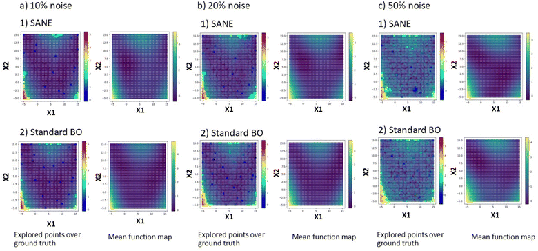 |
| | Fig. 4 Comparison of exploration between BO and SANE on a synthetic 2D search space at (a) 10%, (b) 20% and (c) 50% of random noise from normal distribution. | |
2.2. Implementation in piezoresponse spectroscopy of composition spread combinatorial library Sm-BFO
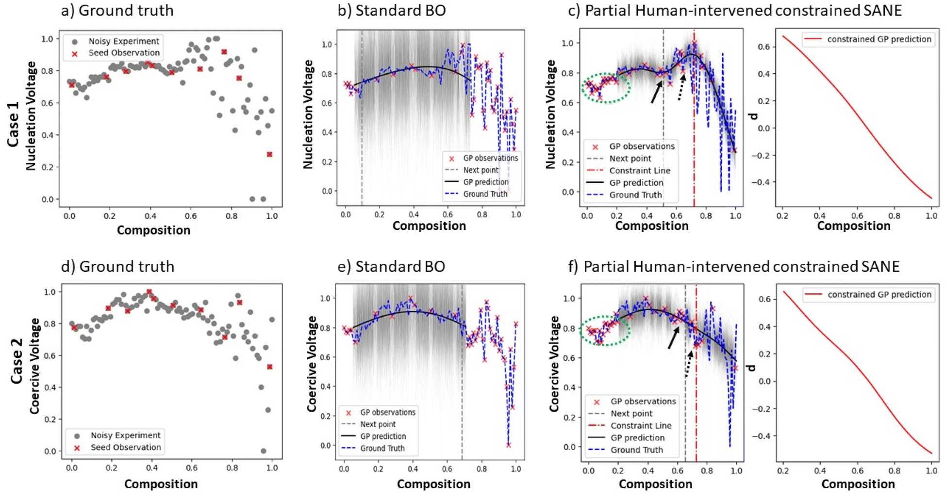
We first implemented the strategic BO in a combinatorial library ferroelectric Sm-doped BiFeO3 (Sm-BFO) dataset.54 Details regarding materials of this dataset have been reported in our previous work.45 Briefly, the dataset, acquired by our AEcroscopy platform55 with a NanoSurf Driven AFM, comprises a spectrum of piezoresponse vs. voltage hysteresis loops across the composition spread of Sm-BFO. Sm-BFO comprises transition with an increase of Sm content from the ferroelectric state BiFeO3 to a non-ferroelectric state of 20% Sm-doped BiFeO3; as such, the hysteresis loops corresponding to 15–20% Sm-doped BFO are mostly closed, without much information regarding ferroelectric characteristics. The input space is the chemical composition of the sample. The sample used in this work is a composition spread combinatorial library sample, which has systematically varied chemical compositions at different locations of the same sample. This creates a system to effectively explore the relationship between chemical composition and material properties. The sample here is a 1D composition spread library (SmxBi1−xFeO3) with varying Sm and Bi ratios. The physical scalarizers extracted from these closed hysteresis loops consist of very high noise, potentially misleading the autonomous discovery. In this example, the non-smoothness of the function arises due to high experimental noise, and is defined as having multi-modal function (multiple optima) and non-differentiability of the function. In this work, we consider two such scalarizers: (1) nucleation voltage and (2) coercive voltage, where we aim to study both independently. The coercive voltage and the nucleation voltage describe distinct aspects of a ferroelectric material's behavior during polarization switching. The coercive voltage is the voltage required to flip the direction of polarization; it corresponds to the voltage on the hysteresis loop where the polarization becomes zero during the switching. The nucleation voltage is the voltage at which the nucleation of reversed domains begins during the polarization switching process; it is typically the voltage at which the switching starts and is often lower than the coercive voltage. Here, we aim to locate regions which have lower values of nucleation and coercive voltages. These parameters are critical for ferroelectric materials as they determine the electric field required to switch the polarization direction and initiate domain formation, which influence the materials' energy efficiency, switching speed, and overall applicability in e.g., memory devices and sensors.
During the initialization of SANE, where the initial samples are chosen from Latin hypercube sampling, we formulate the human knowledge driven constrained gate (refer to eqn (10)–(14)) through voting as shown in Fig. 5a. To attain meaningful scalarizer values of nucleation and coercive voltages, an appropriate spectral structure is necessary (Fig. 5b). Based on this domain knowledge, the assessment of the initial samples has been conducted as per Fig. 4a. We can clearly see the role of human intervention in passing knowledge to the ML policy regarding the feasibility of the experimental results, as the spectrum of the best (over the lowest nucleation voltage) training sample does not form a hysteresis loop to consider a feasible structure. To obtain broad coverage of the parameter space during initialization and thereby better early human assessment, we utilized the Latin hypercube sampling technique instead of random sampling. Here, the prediction models for data ΔD and gate ΔC are considered as Gaussian process (GP) regression models with a Matern kernel function (refer to the ESI†), and the constraint penalty factor is chosen as P = 1000 through exhaustive analysis with different penalty factors. The standard acquisition function u(X) is considered as the Expected Improvement (EI). Here, the switching parameter trajectory is set as si = 0, i < 15 and si = 1, 15 < i ≤ 30, where the total number of iterations, N = 30. Fig. 6 shows the comparison of the autonomous exploration between standard BO and SANE. We can clearly see (Fig. 6b and e) that the pure data-driven BO suggests exploring significantly over the noisy region in the parameter space due to inaccurately measured low values of nucleation and coercive voltages, with insufficient exploitation of the true global region and non-exploitation of the local regions. In SANE, the dynamic gate (Fig. 6c and f) avoids exploration of those human defined infeasible regions and exploits the feasible global region (highlighted by the green dashed circle). We can see that the gate is tuned with more BO iteration (see ESI Fig. S3†). Secondly, we can also see the exploitation of the local regions (pointed with black arrows) aiming to provide deeper insight into the material behavior. One of which would be the understanding of the local robustness of the material behavior, given the physically relevant experimental measurements (feasible spectral structure). For Case 1, in Fig. 6c, we can see a comparison of two local regions of interest; the left local region (pointed by solid black arrow) gives lower nucleation voltage and lower local fluctuation/noise than the right local region (pointed by dashed black arrow). To quantify the SANE performance, here we can see that SANE explores just 1 additional sample over the infeasible noisy region while BO exhausts more than 50% samples over the infeasible region. Also, SANE exploits 3 out of 3 regions of interest (the global region is denoted by the green circle and local regions are denoted by the black arrows) while BO exploits 1 (global) region. Also, BO explores with approx. 5/30 samples in the true feasible region of interest while SANE explores with approx. 26/30 samples in the true region of interest. Case 2 observation has more interesting trade-offs where, in Fig. 6f, we can see a comparison of two local regions of interest. The left local region (indicated by the solid black arrow) gives higher coercive voltage but lower local fluctuation/noise than the right local region (indicated by the dashed black arrow). Also, the right local region is very close to the estimated infeasible space. We can see from the standard BO that this local exploitation has not been suggested within the same cost of exploration, due to being overly exploring on the infeasible region and ignoring potentially interesting local regions. Furthermore, we can observe similar quantitative performance of SANE and BO as in Case 1.
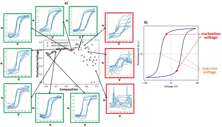 |
| | Fig. 5 Human assessment of the initial samples to define the feasibility of the noisy experiments. In figure (a), the spectral structure images highlighted in green are the positive assessments while the spectral structure images highlighted in red are the negative assessments. These initial samples are generated via the Latin hypercube sampling method. Figure (b) defines the scalarizers such as nucleation and coercive voltages, given the spectral structure of the hysteresis loop. | |
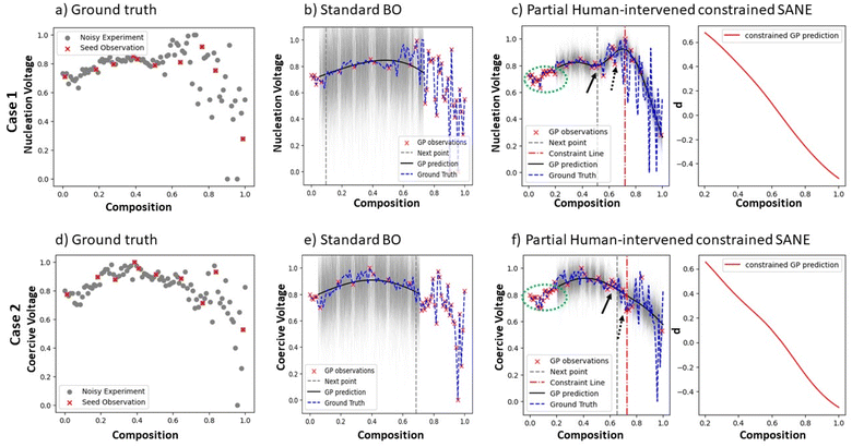 |
| | Fig. 6 Comparison of standard BO and SANE exploration in a combinatorial library ferroelectric Sm-doped BiFeO3 (Sm-BFO) dataset. In Case 1, the objective is the minimization of the nucleation voltage and in Case 2, the objective is the minimization of the coercive voltage. Figures (a) and (d) are the noisy experimental ground truth data for these two cases, where the red dots are the initially LHS-driven selected samples. Figures (b) and (c) are the standard BO and the SANE exploration, respectively, for Case 1, and figures (e) and (f) are the same plots for Case 2, where the black solid lines are the respective estimated mean of the ground truth function, and the black shaded regions are the uncertainty. The red “x” points are the 30 autonomously driven samples for each case study. The red vertical dashed line in the left figures of (c) and (f) are the estimated constraint boundaries or gate = 0 where the left region of the boundary is the feasible region > 0, and the right region of the boundary is the infeasible region < 0. The right figures of (c) and (f) are the estimated constrained gate function with feasible region of > 0. | |
3 Implementation in BEPS PTO data
The second model dataset is the vertical band excitation piezoresponse spectroscopy (BEPS) data of a PbTiO3 (PTO) thin film.46 Here, we aim to locate regions which have higher values of loop area for advanced memory device application. In this example, the non-smoothness of the function, which arises due to high experimental noise, is defined as having multi-modal function (multiple optima). We initialize the SANE with 30 LHS driven initial samples and their domain expert assessments. Here, the prediction models for data ΔD and gate ΔC are considered as deep kernel learning (DKL) regression models56 with Matern kernel and RBF kernel functions (refer to the ESI †), and the constraint penalty factor is chosen as P = 1000. For high dimensionality problems, deep kernel provides better estimation of the structure–property relationship than a standard GP.57 DKL is built on the framework on fully-connected neural network (NN) where the high-dimensional input image patch is first embedded into low dimensional kernel space (in this case set as 2), and then a standard GP kernel operates, such that the parameters of GP and weights of NN are learned jointly. This DKL technique has been implemented for better exploration through active learning in experimental environments.58–62 Here, we utilized a DKL implementation from the open-source Gpax software package. Here, for a selected sample co-ordinate as suggested by the acquisition function, we input a local structure image patch (high dimensional data) to the DKL which predicts the output (loop area). Unlike in the standard GP, through DKL we can provide prior knowledge about the local correlation of the structural image patches. The standard acquisition function u(X) is considered as the Expected Improvement (EI). Here, the switching parameter trajectory is set as si = 0, i < 60 and si = 1, 60 < i ≤ 100, where the total number of iterations, N = 100.
Fig. 7 compares the performance between the standard BO exploration and SANE exploration after 100 iterations. On the SANE exploration, we considered three workflows—(1) without gate, (2) with a relaxed gate and (3) with the hard gate. The relaxed gate is designed with only estimation of the constrained gate map with initial data and is not being updated with selection of new samples. The hard gate is designed as described earlier. The constrained gate maps are provided in ESI Fig. S4.† Comparing with BO, we can clearly see the diversification of the search in all SANE explorations where the standard BO concentrated mostly on a single region (top left boundary of the image space), assuming no potential good solutions can be found in other areas. Whereas all the SANE workflows discover another optimal region (left bottom corner of the image space indicated with red arrow) where we can see the desired spectral structure with a large loop area. Among all the SANE workflows, the relaxed constrained SANE achieves discovery of another optimal region where we can see the desired spectrum (indicated by the red arrow in Fig. 6c) with a large loop area. With further investigation, we understand that the region is very close to infeasibility for the estimated hard gate and is therefore not being explored. SANE explores a lot of infeasible regions over the unconstrained search space and therefore failed to locate the true feasible optimal region. This shows the role of human intervention to reduce the search space and subsequently, intelligent co-navigation to locate the optimal regions in the narrow space. However, we need to ensure the proper balancing of the location of the gates and therefore proper tuning of the penalty factor P is required, which is problem dependent. To quantify the SANE performance, here we can see that all the SANE architectures locate additionally 2–3 optimal regions than the standard BO. To understand that the additional local optimal solutions are truly optimal, we manually investigated the respective spectral structure as shown in the figure, which matches the desirability of the user. Comparing the mean absolute error between the ground truth and the prediction over the estimated feasible space, defined by the hard gate, we can see that SANE has lower error than BO. However, it is to be noted that SANE is not designed to guarantee to always minimize the prediction of the overall feasible multi-modal or non-differentiable parameter space than BO, which is a task for the prediction model. Here, the purpose of SANE is to reduce the over-dependencies of the prediction model and explore strategically to avoid being stuck in a single region and probabilistically hop to explore other regions of interest, when the parameter space is too complex due to noisy experiments. To design or integrate a better predictive model42 to learn a complex non-smooth function is a future scope. Comparing the computational and resource usage among standard BO and different SANE architectures for a fixed experiment, it depends on the number of surrogate predictions for gate mapping. While standard BO and SANE without gate show nearly similar computational cost, the computational cost for SANE with a relaxed gate has one additional surrogate prediction for gate mapping, while the total SANE with the hard gate has double computational cost for gate mapping at every iteration. However, in view of the practical application for autonomous data collection over expensive experiments, the computational cost for an additional gate mapping is negligible in comparison to the cost of a single experiment.
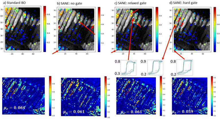 |
| | Fig. 7 Comparison of standard BO and SANE exploration in BEPS data of a PbTiO3 (PTO) thin film: figure (a) is the exploration from standard BO, figure (b) is the SANE exploration without implementation of the human-intervened gate, figure (c) is the SANE exploration with relaxed human-intervened gate, figure (d) is the SANE exploration with hard human-intervened gate. For each subfigure, the top figure is the explored points over the ground truth (loop area) after 100 iterations. The color of the explored points indicates the loop area value where red indicates the higher values (optimal regions) and blue indicates the lower values. The bottom figure is the absolute error map over only the feasible region between the ground truth and the prediction with mean values of μe = 0.064, μe = 0.061, μe = 0.061, μe = 0.059, respectively. | |
For further performance validation of SANE, we compared the histograms between the ground truth and the predictions over the estimated feasible space and compared the ground truth with the explored samples after 100 iterations as in Fig. 8. From the histogram of the ground truth, we can clearly see that the majority of the areas are non-interesting regions with narrow patches of scattered local and global optimal regions. Along with the noisy experiment (fake optima), the low ratio of the true region of interest makes the exploration even harder, like finding a needle in a haystack. It is understandable why standard BO focuses on one region of interest and could not find suitable learning to exploit other regions. Therefore, we can see that it fails to provide a better overall prediction at the estimated feasible region where it has the lowest (ssimBO = 0.217) similarity to the ground truth histogram (refer to Fig. 8a). The similarity index for all the SANE workflows (Fig. 8b–d) are much higher and comparable with each other. From Fig. 7e, we can see that all the SANE workflows overall explore a better ratio of different optimal regions, as they locate a higher percentage of spectral structure having higher loop areas (indicated by the green circle). This is supported by the analysis in Fig. 7 where SANE discovers multiple optimal regions. We can clearly see that BO fails to do so as it mostly explores near the single region of interest and ends up locating spectral structure with loop areas ranging between 0.5 and 0.7. This is because in traditional BO, the acquisition function is built to locate global optima only and does not provide enough priority to exploit local optima, once a global solution is found. Here, the goal of SANE is to maximize the finding of multiple local and global optimal and exploit those with similar priority. Thus, SANE aims to locate more local optima, irrespective of any global solution found. It is to be noted that there could be more local regions which SANE is not able to detect yet with the current number of iterations, and thus more iterations would be required. However, with similar number of iterations, we can easily see better performance of SANE than traditional BO. To understand the role of the gate constraint in this context, as the ground truth of the constraint is unknown, we have run SANE with standard expected improvement acquisition function, but with integrating the gate (see ESI Fig. S5†). We observe that though the gate helps to explore better and locate 1 good region, it also fails to locate another good region as other SANE model did. Additionally, the exploration is concentrated on a particular region and does not exploit the local regions found, which is expected from the standard acquisition. This shows that both the hybrid acquisition and the gate in SANE have roles to play for better guidance of the exploration, particularly when the exploration space contains multiple and fake optima. However, it is to be noted that the dominating factor between them depends on the complexity of the problem.
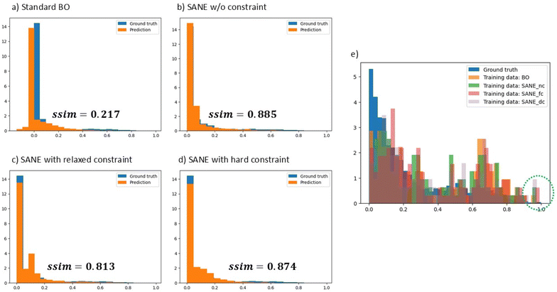 |
| | Fig. 8 Comparison of standard BO and SANE exploration in BEPS data of a PbTiO3 (PTO) thin film. Figures (a)–(d) are the comparison of the histogram between the ground truth and the prediction at the estimated feasible region; driven by standard BO, SANE without implementation of the human-intervened gate, SANE with relaxed human-intervened gate, and SANE with hard human-intervened gate. Figure (e) is the comparison chart of the histograms among ground truth samples (blue), BO-driven samples (orange), SANE without constrained gate driven samples (green), SANE with relaxed constrained gate driven samples (red) and SANE with hard constrained gate driven samples (purple). | |
4 Conclusion
In conclusion, we have developed a Strategic Autonomous Non-Smooth Exploration (SANE) framework, which demonstrates advancements in exploring multidimensional parameter spaces with multi-modal and non-differentiable black box functions for materials and physics discovery. Traditional BO methods, while powerful, often lead to the risk of over-focusing on singular optimal conditions and the potential for becoming trapped in noisy regions or local optima. SANE integrates a cost-driven probabilistic acquisition function, a more robust and exploratory approach, to address these limitations in autonomous experimentation. SANE actively seeks out multiple global and local optima, ensuring a more comprehensive exploration of the parameter space. The application of the SANE framework in two complex material systems, i.e., Sm-doped BiFeO3 combinatorial library and PbTiO3 ferroelastic/ferroelectric thin films, has demonstrated its efficacy. In both cases, SANE outperformed traditional BO by avoiding entrapment in noisy regions and/or singular optimum, enabling the discovery of multiple optimal conditions and uncovering a broader spectrum of material behaviors. Moreover, by incorporating a dynamic constrained gate driven by human domain knowledge, we have further enhanced the SANE framework by prioritizing scientifically valuable regions of the parameter space. Comparing the computation and resource efficiency between SANE and traditional BO, SANE does not provide any significant increment of cost as the cost driven functions are cheap to evaluate and we have limited human intervention till the early initialization stage. As for future tasks, we aim to expand the human intervention in the SANE process with automated triggering of human input for steering based on periodic monitoring of the constraint validation. In future, we also aim to expand SANE to explore over joint multiple functional and fidelity spaces and compare with more advanced BO methods. This approach not only mitigates the challenges posed by experimental noise and uncertainties but also ensures that the exploration aligns with broader scientific discovery goals.
As autonomous experimentation for accelerated research continues to evolve, the integration of advanced autonomous exploration methods like SANE, coupled with human expertise, will stand as a critical tool for pushing the boundaries of what is possible in autonomous research, more comprehensive explorations of complex material landscapes and driving new scientific discoveries. The approach developed here can be applied in a broad materials science field including materials synthesis, characterization, and computation, offering a more comprehensive and effective path forward in autonomous research.
Data availability
The analysis reported here along with the code is summarized in Colab Notebook for the purpose of tutorial and application to other data and can be found at https://github.com/arpanbiswas52/SANE.
Author contributions
A. B. and Y. L. conceived the project. A. B. developed the SANE framework. Y. L and R. V developed the AEcroscopy platform for data acquisition. Y. L. acquired the experimental data for SANE investigation and A. B. performed the analysis. R. P and I. T prepared the Sm-doped BiFeO3 sample. H. F. prepared the PbTiO3 (PTO) thin film sample. A. B. and Y. L. wrote the manuscript. All authors edited the manuscript.
Conflicts of interest
The authors confirm no conflicts of interest.
Acknowledgements
A. B. was supported by the University of Tennessee startup funding. The authors acknowledge the use of facilities and instrumentation at the UT Knoxville Institute for Advanced Materials and Manufacturing (IAMM) and the Shull Wollan Center (SWC) supported in part by the National Science Foundation Materials Research Science and Engineering Center program through the UT Knoxville Center for Advanced Materials and Manufacturing (DMR-2309083). This research (domain knowledge intergration) sponsored by the INTERSECT Initiative as part of the Laboratory Directed Research and Development Program of Oak Ridge National Laboratory, managed by UT-Battelle, LLC for the US Department of Energy under contract DE-AC05-00OR22725. This effort (PFM datasets) was supported by the Center for Nanophase Materials Sciences (CNMS), which is a US Department of Energy, Office of Science User Facility at Oak Ridge National Laboratory. R. V. and I. T. were supported by the US Department of Energy, Office of Science, Office of Basic Energy Sciences Energy Frontier Research Centers program under Award Number DE-SC0021118. H. F. was supported by the Japan Science and Technology Agency (JST) as part of Adopting Sustainable Partnerships for Innovative Research Ecosystem (ASPIRE), Grant Number JPMJAP2312.
References
- M. Abolhasani and E. Kumacheva, The Rise of Self-Driving Labs in Chemical and Materials Sciences, Nat. Synth., 2023, 2(6), 483–492, DOI:10.1038/s44160-022-00231-0.
- S. V. Kalinin, M. Ziatdinov, J. Hinkle, S. Jesse, A. Ghosh, K. P. Kelley, A. R. Lupini, B. G. Sumpter and R. K. Vasudevan, Automated and Autonomous Experiments in Electron and Scanning Probe Microscopy, ACS Nano, 2021, 15(8), 12604–12627, DOI:10.1021/acsnano.1c02104.
- E. Stach, B. DeCost, A. G. Kusne, J. Hattrick-Simpers, K. A. Brown, K. G. Reyes, J. Schrier, S. Billinge, T. Buonassisi, I. Foster, C. P. Gomes, J. M. Gregoire, A. Mehta, J. Montoya, E. Olivetti, C. Park, E. Rotenberg, S. K. Saikin, S. Smullin, V. Stanev and B. Maruyama, Autonomous Experimentation Systems for Materials Development: A Community Perspective, Matter, 2021, 4(9), 2702–2726, DOI:10.1016/j.matt.2021.06.036.
-
G. Tom, S. P. Schmid, S. G. Baird, Y. Cao, K. Darvish, H. Hao, S. Lo, S. Pablo-García, E. M. Rajaonson, M. Skreta, N. Yoshikawa, S. Corapi, G. D. Akkoc, F. Strieth-Kalthoff, M. Seifrid andA. Aspuru-Guzik, Self-Driving Laboratories for Chemistry and Materials Science, ChemRxiv, 2024, preprint, DOI:10.26434/chemrxiv-2024-rj946-v2.
- Y. Xie, K. Sattari, C. Zhang and J. Lin, Toward Autonomous Laboratories: Convergence of Artificial Intelligence and Experimental Automation, Prog. Mater. Sci., 2023, 132, 101043, DOI:10.1016/j.pmatsci.2022.101043.
- B. Shahriari, K. Swersky, Z. Wang, R. P. Adams and N. de Freitas, Taking the Human Out of the Loop: A Review of Bayesian Optimization, Proc. IEEE, 2016, 104(1), 148–175, DOI:10.1109/JPROC.2015.2494218.
- D. R. Jones, M. Schonlau and W. J. Welch, Efficient Global Optimization of Expensive Black-Box Functions, J. Glob. Optim., 1998, 13(4), 455–492, DOI:10.1023/A:1008306431147.
- A. Biswas and C. Hoyle, An Approach to Bayesian Optimization for Design Feasibility Check on Discontinuous Black-Box Functions, J. Mech. Des., 2021, 143, 031716, DOI:10.1115/1.4049742.
-
N. Quadrianto, K. Kersting and Z. Xu, Gaussian Process, in Encyclopedia of Machine Learning, ed. Sammut, C. and Webb, G. I., Springer US, Boston, MA, 2010; pp pp 428–439, DOI:10.1007/978-0-387-30164-8_324.
- V. L. Deringer, A. P. Bartók, N. Bernstein, D. M. Wilkins, M. Ceriotti and G. Csányi, Gaussian Process Regression for Materials and Molecules, Chem. Rev., 2021, 121(16), 10073–10141, DOI:10.1021/acs.chemrev.1c00022.
- M. M. Noack, G. S. Doerk, R. Li, J. K. Streit, R. A. Vaia, K. G. Yager and M. Fukuto, Autonomous Materials Discovery Driven by Gaussian Process Regression with Inhomogeneous Measurement Noise and Anisotropic Kernels, Sci. Rep., 2020, 10(1), 17663, DOI:10.1038/s41598-020-74394-1.
-
E. Brochu, V. M. Cora and N. de Freitas, A Tutorial on Bayesian Optimization of Expensive Cost Functions, with Application to Active User Modeling and Hierarchical Reinforcement Learning, arXiv, 2010, preprint, arXiv:1012.2599, DOI:10.48550/arXiv.1012.2599.
-
D. D. Cox and S. John, A Statistical Method for Global Optimization, in Proceedings 1992 IEEE International Conference on Systems, Man, and Cybernetics, 1992, vol. 2, pp 1241–1246, DOI:10.1109/ICSMC.1992.271617.
- D. R. Jones, A Taxonomy of Global Optimization Methods Based on Response Surfaces, J. Glob. Optim., 2001, 21(4), 345–383, DOI:10.1023/A:1012771025575.
- H. J. Kushner, A New Method of Locating the Maximum Point of an Arbitrary Multipeak Curve in the Presence of Noise, J. Basic Eng., 1964, 86(1), 97–106, DOI:10.1115/1.3653121.
- S. L. Sanchez, E. Foadian, M. Ziatdinov, J. Yang, S. V. Kalinin, Y. Liu and M. Ahmadi, Physics-Driven Discovery and Bandgap Engineering of Hybrid Perovskites, Digit. Discov., 2024, 3(8), 1577–1590, 10.1039/D4DD00080C.
- J. Chang, P. Nikolaev, J. Carpena-Núñez, R. Rao, K. Decker, A. E. Islam, J. Kim, M. A. Pitt, J. I. Myung and B. Maruyama, Efficient Closed-Loop Maximization of Carbon Nanotube Growth Rate Using Bayesian Optimization, Sci. Rep., 2020, 10(1), 9040, DOI:10.1038/s41598-020-64397-3.
- T. Ueno, T. D. Rhone, Z. Hou, T. Mizoguchi and K. Tsuda, COMBO: An Efficient Bayesian Optimization Library for Materials Science, Mater. Discov., 2016, 4, 18–21, DOI:10.1016/j.md.2016.04.001.
- S. V. Kalinin, M. Ziatdinov and R. K. Vasudevan, Guided Search for Desired Functional Responses via Bayesian Optimization of Generative Model: Hysteresis Loop Shape Engineering in Ferroelectrics, J. Appl. Phys., 2020, 128(2), 024102, DOI:10.1063/5.0011917.
- A. Biswas, A. N. Morozovska, M. Ziatdinov, E. A. Eliseev and S. V. Kalinin, Multi-Objective Bayesian Optimization of Ferroelectric Materials with Interfacial Control for Memory and Energy Storage Applications, J. Appl. Phys., 2021, 130(20), 204102, DOI:10.1063/5.0068903.
- A. N. Morozovska, E. A. Eliseev, A. Biswas, H. V. Shevliakova, N. V. Morozovsky and S. V. Kalinin, Chemical Control of Polarization in Thin Strained Films of a Multiaxial Ferroelectric: Phase Diagrams and Polarization Rotation, Phys. Rev. B, 2022, 105(9), 094112, DOI:10.1103/PhysRevB.105.094112.
- A. N. Morozovska, E. A. Eliseev, A. Biswas, N. V. Morozovsky and S. V. Kalinin, Effect of Surface Ionic Screening on Polarization Reversal and Phase Diagrams in Thin Antiferroelectric Films for Information and Energy Storage, Phys. Rev. Appl., 2021, 16(4), 044053, DOI:10.1103/PhysRevApplied.16.044053.
- S. Tao, A. van Beek, D. W. Apley and W. Chen, Multi-Model Bayesian Optimization for Simulation-Based Design, J. Mech. Des., 2021, 143, 111701, DOI:10.1115/1.4050738.
- G. Narasimha, S. Hus, A. Biswas, R. Vasudevan and M. Ziatdinov, Autonomous Convergence of STM Control Parameters Using Bayesian Optimization, APL Mach. Learn., 2024, 2(1), 016121, DOI:10.1063/5.0185362.
- Y. Liu, K. P. Kelley, R. K. Vasudevan, H. Funakubo, M. A. Ziatdinov and S. V. Kalinin, Experimental Discovery of Structure–Property Relationships in Ferroelectric Materials via Active Learning, Nat. Mach. Intell., 2022, 4(4), 341–350, DOI:10.1038/s42256-022-00460-0.
- R.-R. Griffiths and J. M. Hernández-Lobato, Constrained Bayesian Optimization for Automatic Chemical Design Using Variational Autoencoders, Chem. Sci., 2020, 11(2), 577–586, 10.1039/C9SC04026A.
- B. Burger, P. M. Maffettone, V. V. Gusev, C. M. Aitchison, Y. Bai, X. Wang, X. Li, B. M. Alston, B. Li, R. Clowes, N. Rankin, B. Harris, R. S. Sprick and A. I. Cooper, A Mobile Robotic Chemist, Nature, 2020, 583(7815), 237–241, DOI:10.1038/s41586-020-2442-2.
- A. G. Kusne, H. Yu, C. Wu, H. Zhang, J. Hattrick-Simpers, B. DeCost, S. Sarker, C. Oses, C. Toher, S. Curtarolo, A. V. Davydov, R. Agarwal, L. A. Bendersky, M. Li, A. Mehta and I. Takeuchi, On-the-Fly Closed-Loop Materials Discovery via Bayesian Active Learning, Nat. Commun., 2020, 11(1), 5966, DOI:10.1038/s41467-020-19597-w.
- A. Dave, J. Mitchell, S. Burke, H. Lin, J. Whitacre and V. Viswanathan, Autonomous Optimization of Non-Aqueous Li-Ion Battery Electrolytes via Robotic Experimentation and Machine Learning Coupling, Nat. Commun., 2022, 13(1), 5454, DOI:10.1038/s41467-022-32938-1.
- S. B. Harris, A. Biswas, S. J. Yun, K. M. Roccapriore, C. M. Rouleau, A. A. Puretzky, R. K. Vasudevan, D. B. Geohegan and K. Xiao, Autonomous Synthesis of Thin Film Materials with Pulsed Laser Deposition Enabled by In Situ Spectroscopy and Automation, Small Methods, 2301763, DOI:10.1002/smtd.202301763.
- K. J. Kanarik, W. T. Osowiecki, Y. Lu (Joe), D. Talukder, N. Roschewsky, S. N. Park, M. Kamon, D. M. Fried and R. A. Gottscho, Human–Machine Collaboration for Improving Semiconductor Process Development, Nature, 2023, 616(7958), 707–711, DOI:10.1038/s41586-023-05773-7.
- A. Biswas, Y. Liu, N. Creange, Y.-C. Liu, S. Jesse, J.-C. Yang, S. V. Kalinin, M. A. Ziatdinov and R. K. Vasudevan, A Dynamic Bayesian Optimized Active Recommender System for Curiosity-Driven Partially Human-in-the-Loop Automated Experiments, npj Comput. Mater., 2024, 10(1), 1–12, DOI:10.1038/s41524-023-01191-5.
-
A. Biswas, Y. Liu, M. Ziatdinov, Y.-C. Liu, S. Jesse, J.-C. Yang, S. Kalinin and R. Vasudevan, A Multi-Objective Bayesian Optimized Human Assessed Multi-Target Generated Spectral Recommender System for Rapid Pareto Discoveries of Material Properties, American Society of Mechanical Engineers Digital Collection, 2023, DOI:10.1115/DETC2023-116956.
- Y. Liu, M. A. Ziatdinov, R. K. Vasudevan and S. V. Kalinin, Explainability and Human Intervention in Autonomous Scanning Probe Microscopy, Patterns, 2023, 4(11), 100858, DOI:10.1016/j.patter.2023.100858.
- S. V. Kalinin, Y. Liu, A. Biswas, G. Duscher, U. Pratiush, K. Roccapriore, M. Ziatdinov and R. Vasudevan, Human-in-the-Loop: The Future of Machine Learning in Automated Electron Microscopy, Microsc. Today, 2024, 32(1), 35–41, DOI:10.1093/mictod/qaad096.
- S. B. Harris, R. Vasudevan and Y. Liu, Active oversight and quality control in standard Bayesian optimization for autonomous experiments, npj Comput. Mater., 2023, 11, 23, DOI:10.1038/s41524-024-01485-2.
- A. Biswas, M. Valleti, R. Vasudevan, M. Ziatdinov and S. V. Kalinin, Toward Accelerating Discovery via Physics-Driven and Interactive Multifidelity Bayesian Optimization, J. Comput. Inf. Sci. Eng., 2024, 24(12), 121005, DOI:10.1115/1.4066856.
-
R. Garnett, Bayesian Optimization, Cambridge Core, DOI:10.1017/9781108348973.
-
M. Balandat, B. Karrer, D. R. Jiang, S. Daulton, B. Letham, A. G. Wilson and E. Bakshy, BOTORCH: A Framework for Efficient Monte-Carlo Bayesian Optimization, in Proceedings of the 34th International Conference on Neural Information Processing Systems; NIPS'20, Curran Associates Inc., Red Hook, NY, USA, 2020, pp 21524–21538 Search PubMed.
- M. A. Ziatdinov, Y. Liu, A. N. Morozovska, E. A. Eliseev, X. Zhang, I. Takeuchi and S. V. Kalinin, Hypothesis Learning in Automated Experiment: Application to Combinatorial Materials Libraries, Adv. Mater., 2022, 34(20), 2201345, DOI:10.1002/adma.202201345.
- M. Gaudioso, G. Giallombardo and G. Miglionico, Essentials of Numerical Nonsmooth Optimization, Ann. Oper. Res., 2022, 314(1), 213–253, DOI:10.1007/s10479-021-04498-y.
- H Luo, Y. Cho, J. W. Demmel, I. Kozachenko, X. S. Li and Y. Liu, Non-smooth Bayesian optimization in tuning scientific applications, Int. J. High Perform. Comput. Appl., 2024, 38(6), 633–657, DOI:10.1177/10943420241278981.
- D. Ramachandram, M. Lisicki, T. J. Shields, M. R. Amer and G. W. Taylor, Bayesian Optimization on Graph-Structured Search Spaces: Optimizing Deep Multimodal Fusion Architectures, Neurocomputing, 2018, 298, 80–89, DOI:10.1016/j.neucom.2017.11.071.
- B. N. Slautin, U. Pratiush, I. N. Ivanov, Y. Liu, R. Pant, X. Zhang, I. Takeuchi, M. A. Ziatdinov and S. V. Kalinin, Co-Orchestration of Multiple Instruments to Uncover Structure-Property Relationships in Combinatorial Libraries, Digit. Discov., 2024, 3(8), 1602–1611, 10.1039/D4DD00109E.
- A. Raghavan, R. Pant, I. Takeuchi, E. A. Eliseev, M. Checa, A. N. Morozovska, M. Ziatdinov, S. V. Kalinin and Y. Liu, Evolution of Ferroelectric Properties in SmxBi1-xFeO3 via Automated Piezoresponse Force Microscopy across Combinatorial Spread Libraries, ACS Nano, 2024, 18(37), 25591–25600, DOI:10.1021/acsnano.4c06380.
- U. Pratiush, H. Funakubo, R. Vasudevan, S. V. Kalinin and Y. Liu, Scientific Exploration with Expert Knowledge (SEEK) in Autonomous Scanning Probe Microscopy with Active Learning, Digital Discovery, 2025, 4(1), 252–263, 10.1039/D4DD00277F.
-
D. Eriksson, M. Pearce, J. Gardner, R. D. Turner and M. Poloczek, Scalable Global Optimization via Local Bayesian Optimization, in Advances in Neural Information Processing Systems, Curran Associates, Inc., 2019, vol. 32 Search PubMed.
- P. Luong, D. Nguyen, S. Gupta, S. Rana and S. Venkatesh, Adaptive Cost-Aware Bayesian Optimization, Knowl.-Based Syst., 2021, 232, 107481, DOI:10.1016/j.knosys.2021.107481.
- R. Liang, H. Hu, Y. Han, B. Chen and Z. Yuan, CAPBO: A Cost-Aware Parallelized Bayesian Optimization Method for Chemical Reaction Optimization, AIChE J., 2024, 70(3), e18316, DOI:10.1002/aic.18316.
-
E. H. Lee, V. Perrone, C. Archambeau and M. Seeger, Cost-Aware Bayesian Optimization, arXiv, 2020, preprint, arXiv:2003.10870, DOI:10.48550/arXiv.2003.10870.
- B. N. Slautin, Y. Liu, H. Funakubo, R. K. Vasudevan, M. Ziatdinov and S. V. Kalinin, Bayesian Conavigation: Dynamic Designing of the Material Digital Twins via Active Learning, ACS Nano, 2024, 18, 24898–24908, DOI:10.1021/acsnano.4c05368.
- B. N. Slautin, Y. Liu, H. Funakubo and S. V. Kalinin, Unraveling the Impact of Initial Choices and In-Loop Interventions on Learning Dynamics in Autonomous Scanning Probe Microscopy, J. Appl. Phys., 2024, 135(15), 154901, DOI:10.1063/5.0198316.
-
Branin Function, https://www.sfu.ca/%7Essurjano/branin.html, accessed 2024-08-30.
- S. Fujino, M. Murakami, V. Anbusathaiah, S.-H. Lim, V. Nagarajan, C. J. Fennie, M. Wuttig, L. Salamanca-Riba and I. Takeuchi, Combinatorial Discovery of a Lead-Free Morphotropic Phase Boundary in a Thin-Film Piezoelectric Perovskite, Appl. Phys. Lett., 2008, 92(20), 202904, DOI:10.1063/1.2931706.
- Y. Liu, K. Roccapriore, M. Checa, S. M. Valleti, J.-C. Yang, S. Jesse and R. K. Vasudevan, AEcroscopy: A Software–Hardware Framework Empowering Microscopy Toward Automated and Autonomous Experimentation, Small Methods, 2301740, DOI:10.1002/smtd.202301740.
-
A. G. Wilson, Z. Hu, R. Salakhutdinov and E. P. Xing, Deep Kernel Learning, in, Proc. 19th International Conference on Artificial Intelligence and Statistics, ed. N. Lawrence, Proceedings of Machine Learning Research (PMLR), 2016, vol. 51, pp. 370–378 Search PubMed.
- M. Ziatdinov, A. Ghosh, C. Y. Wong (Tommy) and S. V. Kalinin, AtomAI Framework for Deep Learning Analysis of Image and Spectroscopy Data in Electron and Scanning Probe Microscopy, Nat. Mach. Intell., 2022, 4(12), 1101–1112, DOI:10.1038/s42256-022-00555-8.
- K. M. Roccapriore, S. V. Kalinin and M. Ziatdinov, Physics Discovery in Nanoplasmonic Systems via Autonomous Experiments in Scanning Transmission Electron Microscopy, Adv. Sci., 2022, 9(36), 2203422, DOI:10.1002/advs.202203422.
-
M. Ziatdinov, Y. Liu and S. V. Kalinin, Active Learning in Open Experimental Environments: Selecting the Right Information Channel(s) Based on Predictability in Deep Kernel Learning, arXiv, 2022, preprint, arXiv:2203.10181, DOI:10.48550/arXiv.2203.10181.
- Y. Liu, K. P. Kelley, R. K. Vasudevan, W. Zhu, J. Hayden, J.-P. Maria, H. Funakubo, M. A. Ziatdinov, S. Trolier-McKinstry and S. V. Kalinin, Automated Experiments of Local Non-Linear Behavior in Ferroelectric Materials, Small, 2022, 18(48), 2204130, DOI:10.1002/smll.202204130.
- Y. Liu, K. P. Kelley, R. K. Vasudevan, H. Funakubo, M. A. Ziatdinov and S. V. Kalinin, Experimental Discovery of Structure–Property Relationships in Ferroelectric Materials via Active Learning, Nat. Mach. Intell., 2022, 4(4), 341–350, DOI:10.1038/s42256-022-00460-0.
- Y. Liu, R. K. Vasudevan, K. P. Kelley, H. Funakubo, M. Ziatdinov and S. V. Kalinin, Learning the Right Channel in Multimodal Imaging: Automated Experiment in Piezoresponse Force Microscopy, npj Comput. Mater., 2023, 9, 34, DOI:10.1038/s41524-023-00985-x.
|
| This journal is © The Royal Society of Chemistry 2025 |
Click here to see how this site uses Cookies. View our privacy policy here. 
 Open Access Article
 This Open Access Article is licensed under a
  a,
Rama
Vasudevan
a,
Rama
Vasudevan