Monitoring wind and particle concentrations near freshwater and marine harmful algal blooms (HABs)

Abstract

Harmful algal blooms (HABs) are a threat to aquatic ecosystems worldwide. New information is needed about the environmental conditions associated with the aerosolization and transport of HAB cells and their associated toxins. This information is critical to help inform our understanding of potential exposures. We used a ground-based sensor package to monitor weather, measure airborne particles, and collect air samples on the shore of a freshwater HAB (bloom of predominantly Rhaphidiopsis, Lake Anna, Virginia) and a marine HAB (bloom of Karenia brevis, Gulf Coast, Florida). Each sensor package contained a sonic anemometer, impinger, and optical particle counter. A drone was used to measure vertical profiles of windspeed and wind direction at the shore and above the freshwater HAB. At the Florida sites, airborne particle number concentrations (cm⁻³) increased throughout the day and the wind direction (offshore versus onshore) was strongly associated with these particle number concentrations (cm⁻³). Offshore wind sources had particle number concentrations (cm⁻³) 3 to 4 times higher than those of onshore wind sources. A predictive model, trained on a random set of weather and particle number concentrations (cm⁻³) collected over the same time period, was able to predict airborne particle number concentrations (cm⁻³) with an R squared value of 0.581 for the freshwater HAB in Virginia and an R squared value of 0.804 for the marine HAB in Florida. The drone-based vertical profiles of the wind velocity showed differences in wind speed and direction at different altitudes, highlighting the need for wind measurements at multiple heights to capture environmental conditions driving the atmospheric transport of aerosolized HAB toxins. A surface flux equation was used to determine the rate of aerosol production at the beach sites based on the measured particle number concentrations (cm⁻³) and weather conditions. Additional work is needed to better understand the short-term fate and transport of aerosolized cyanobacterial cells and toxins and how this is influenced by local weather conditions.

---

Environmental significance

Harmful algal blooms (HABs), often caused by toxic cyanobacteria, are increasingly common phenomena affecting aquatic ecosystems around the world. There is a significant knowledge gap regarding atmospheric transport of HAB cells and toxins. Research is needed to better understand drivers of HAB aerosol emissions and transport, as well as improve monitoring and mitigation when HAB-associated aerosols may endanger the health of domestic animals and humans. Here, we describe the use of ground and aerial sensors to monitor particles and weather conditions over land and water. Models for sea-shore and lake-shore conditions were created to predict particle levels based on different weather conditions. This information could allow for health advisories to be applied at known HAB sites when weather conditions predict higher levels of aerosols, with the potential to improve the quality of life for those who occupy and/or use beaches or lakes for recreational activities.

1. Introduction

Freshwater and marine ecosystems are experiencing an increasing number of harmful algal blooms (HABs).¹ HABs often result from the proliferation of toxin-producing microorganisms that are harmful to humans and wildlife.^2–5 HABs known as red tides may occur in marine environments, and aerosolized toxins from blooms of red tide are known to have harmful impacts on people.^6,7 HABs in lake systems often occur in areas with warmer water and high levels of phosphorus favorable to cyanobacterial growth.^8–10 HABs in oceans may be increasing in frequency as a result of increased monitoring efforts, potential human influences, and ocean acidification.^8,11–14 Potential increases in lake and ocean HAB occurrences are concerning from human and animal health perspectives, and require further study involving higher resolution observations.^1,12,15

Research is needed to better understand how to address and mitigate the impacts of HAB threats to shorelines and downwind impact areas.^16,17 HAB signatures can be seen in samples collected at long distances from the shores of lakes and oceans, indicating the potential for HAB-associated aerosols to influence air quality beyond just the water's edge.^16,18 HABs have also been linked to increased PM_2.5 concentrations, suggesting that HAB-associated aerosols may spread inland from their sources.¹⁹ Generally, water samples are collected by hand from boats and processed at off-site laboratories.²⁰ Recently, robots have presented new opportunities to sample HABs with minimal human exposure.^21,22 Such approaches can be used to inform health guidelines and policy around HAB occurrences to best keep exposure risks low.^4,23,24 The negative economic impact of HABs can also be mitigated through the use of predictive models providing a benefit to the individuals of impacted communities.²⁵

Small uncrewed aircraft systems (sUASs or drones) have been used to monitor HABs and assess their potential impact on surrounding communities.^21,26,27 Technologies with sUASs offer the possibility of sampling the atmosphere in remote, dangerous, and hard-to-reach environments.^28,29 Early applications of sUAS for HAB monitoring involved integrating cameras on board fixed- and rotary-wing sUAS for image data collection.³⁰ More recently, sUAS techniques have been developed to sample both air and water affected by HABs. Hanlon et al.²² used a drone water sampling system to collect water samples from three lakes with HABs. Bilyeu et al.²¹ used an airborne drone particle-monitoring system (AirDROPS) to monitor, collect, and characterize airborne particles over two HABs. González-Rocha et al.²⁷ extended a model-based (sensor free) wind estimation technique to measure atmospheric flows in the airshed of aquatic environments.^26,31

Though mechanisms of aerosolization in marine and freshwater environments have received considerable attention,⁶ new information is needed to understand the environmental factors driving high counts of aerosolized HAB cells and toxins.^10,32–34 We hypothesized that wind direction and speed impact airborne particle concentration differently in marine vs. freshwater systems. This hypothesis is based in part on observations that aerosolization processes are influenced by salinity.^32,33 To test this hypothesis, we conducted drone-based and ground-based sampling missions on the shore of a freshwater HAB (bloom of Rhaphidiopsis, Lake Anna, Virginia) and a marine HAB (bloom of Karenia brevis, Gulf Coast, Florida). The specific objectives of our work were to: (1) monitor airborne particles on the shore of a freshwater HAB (bloom of Rhaphidiopsis, Lake Anna, Virginia) and a marine HAB (bloom of Karenia brevis, Gulf Coast, Florida), (2) observe and model potential associations of wind direction, wind speed, and temperature with airborne particle number concentrations (cm⁻³), and (3) determine onshore and offshore wind profiles at the freshwater HAB site using a small drone platform.

2. Methods and materials

2.1 Study sites

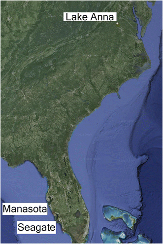
Studies were conducted along the shore of a freshwater HAB at Lake Anna, Virginia, and a marine HAB along the Gulf Coast of Florida (Fig. 1). Lake Anna is a reservoir lake in North-Central Virginia of 13 000 acres and is the third largest lake in the state.³⁵ Our first sampling site was near the inflow of Pamunkey Creek into Lake Anna (site 1; 38.1413, −77.9276). The second sampling site on Lake Anna was on the end of a peninsula between the inflows of Gold Mine Creek and Hickory Creek (site 2; 38.1154, −77.9414). Both locations are in the Northwest portion of the lake and were chosen as a sample site due to HAB observations and reports from the Virginia Department of Health (VDH) of concentrations of potentially toxic cyanobacteria in the lake³⁵ (ESI Table S1 and Fig. S1 and S2†). Ground-based sensors were placed on the shoreline within 5–10 meters of the lake or ocean shore (Table 1). Drone measurements were taken over land as well as over the water surface (Table 2 and Fig. 2). Two ground-based devices were deployed simultaneously at Lake Anna, Virginia for multiple sampling periods (at least 30 minutes each). Two sampling periods were conducted on June 30th, 2020, seven sampling periods were conducted on July 7th, 2020, and four sampling periods were conducted on July 8th, 2020. Wind profiles were performed at Lake Anna following a 30 minute cadence, on average.

Fig. 1 One sampling location at Lake Anna, VA marked in yellow, and the two beaches in Manasota, FL and Seagate, FL in red are marked where sampling was performed. Lake Anna consisted of ground level and drone-based sampling, while Manasota and Seagate beaches consisted of only ground level sampling.

Table 1 Details including the date, time, location, and description (ocean in Florida, lake in Virginia) for each sampling period of the ground-based observations

Date	Start	End	Latitude	Longitude	Description
12/3/2019	11:15	11:45	26.2084	−81.8169	Ocean
12/3/2019	12:00	12:30	26.2084	−81.8169	Ocean
12/3/2019	12:45	13:15	26.2084	−81.8169	Ocean
12/3/2019	13:30	14:00	26.2084	−81.8169	Ocean
12/3/2019	14:15	14:45	26.2084	−81.8169	Ocean
12/3/2019	15:00	15:30	26.2084	−81.8169	Ocean
12/4/2019	9:45	10:15	27.0112	−82.4135	Ocean
12/4/2019	10:30	11:00	27.0112	−82.4135	Ocean
12/4/2019	11:15	11:45	27.0112	−82.4135	Ocean
12/4/2019	12:00	12:30	27.0112	−82.4135	Ocean
12/4/2019	12:45	13:15	27.0112	−82.4135	Ocean
12/4/2019	13:30	14:00	27.0112	−82.4135	Ocean
6/30/2020	10:15	11:00	38.1416	−77.9274	Lake
6/302020	11:15	11:45	38.1416	−77.9274	Lake
7/7/2020	9:15	9:50	38.1413	−77.9276	Lake
7/7/2020	9:55	10:25	38.1413	−77.9276	Lake
7/7/2020	10:35	11:05	38.1413	−77.9276	Lake
7/7/2020	11:20	11:30	38.1413	−77.9276	Lake
7/7/2020	12:00	12:30	38.1413	−77.9276	Lake
7/7/2020	12:45	13:20	38.1413	−77.9276	Lake
7/7/2020	13:35	14:05	38.1413	−77.9276	Lake
7/8/2020	10:40	11:10	38.1154	−77.9415	Lake
7/8/2020	11:25	11:55	38.1154	−77.9415	Lake
7/8/2020	12:05	12:35	38.1154	−77.9415	Lake
7/8/2020	12:45	13:15	38.1154	−77.9415	Lake

---

Table 2 Details including the date, time, maximum altitude, location, and onshore or offshore designation of profile for the drone-based meteorological observations

Date	Start	End	Height (m)	Latitude	Longitude	Description
7/7/2020	9:21	9:23	80	38.1410	−77.9281	Offshore
7/7/2020	9:23	9:26	80	38.1411	−77.9273	Onshore
7/7/2020	9:58	10:00	80	38.1410	−77.9281	Offshore
7/7/2020	10:00	10:02	80	38.1411	−77.9273	Onshore
7/7/2020	10:35	10:37	80	38.1410	−77.9281	Offshore
7/7/2020	10:37	10:40	80	38.1411	−77.9273	Onshore
7/7/2020	10:55	10:58	80	38.1410	−77.9281	Offshore
7/7/2020	10:58	11:00	80	38.1411	−77.9273	Onshore
7/7/2020	11:21	11:24	80	38.1410	−77.9281	Offshore
7/7/2020	11:24	11:26	80	38.1411	−77.9273	Onshore
7/7/2020	11:42	11:44	80	38.1410	−77.9281	Offshore
7/7/2020	11:44	11:46	80	38.1411	−77.9273	Onshore
7/7/2020	‘12:00	12:02	80	38.1410	−77.9281	Offshore
7/7/2020	12:02	12:05	80	38.1411	−77.9273	Onshore
7/7/2020	12:19	12:22	80	38.1410	−77.9281	Offshore
7/7/2020	12:22	12:24	80	38.1411	−77.9273	Onshore
7/7/2020	13:09	13:12	80	38.1410	−77.9281	Offshore
7/7/2020	13:12	13:15	80	38.1411	−77.9273	Onshore
7/7/2020	13:40	13:42	80	38.1410	−77.9281	Offshore
7/7/2020	13:42	13:44	80	38.1411	−77.9273	Onshore
7/7/2020	13:58	14:01	80	38.1410	−77.9281	Offshore
7/7/2020	14:01	14:03	80	38.1411	−77.9273	Onshore

---

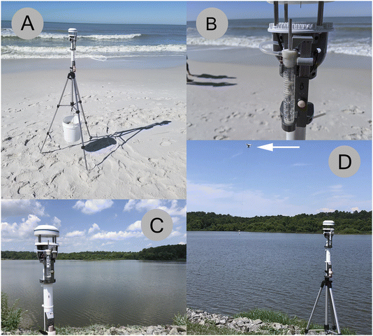Fig. 2 (A) Ground sampling device located at Seagate Beach FL, December 3, 2019. (B) Impinger actively sampling the air while the weather station is running in Florida. (C) Ground sampling device at Lake Anna, Virginia collecting near the lake shore on June 30, 2020. (D) Combined drone (white arrow) and ground sampling at Lake Anna.

The Gulf of Mexico experiences intermittent HABs caused by K. brevis which makes the Florida Gulf coast a prime location for HAB aerosol sampling.⁶ Ground-based sensor sampling was chosen for this location by using the Mote beach conditions reporting system and next-day forecasting from a data-driven model⁷ to determine a beach with a high probability of HAB irritation.³⁶ Seagate beach was chosen as a site, located at GPS coordinates 26.2084, −81.8168 (ESI Fig. S2†). To capture samples earlier in the morning, Manasota beach was chosen for our second sample location. This site was located at GPS coordinates 27.0112, −82.4134 (ESI Fig. S2†). Two sampling devices were used simultaneously for 30 minute sampling periods. Six sampling periods were performed each day on December 3rd and 4th, 2019, at Seagate and Manasota Beach, respectively. A total of 24 beach weather and particle count measurements were collected during this period.

Fourteen sampling periods were conducted along the Gulf of Mexico coast in Florida, and 11 were conducted at Lake Anna in Virginia (Table 1). Sampling periods consisted of ground sensors measuring weather and particle number concentrations (cm⁻³) approximately 2 meters above ground level near to the shore at all sites (Table 1). Drone flights were performed during the Lake Anna sampling periods, both above the shore and above the water alternately, over a range of elevation from 10 to 80 m to measure the wind speed and direction at different altitudes (Table 2). Water samples were collected by hand from both the Florida and Virginia sites, and analyzed using an Imaging Cytometer (Amnis ImageStream MarkII) as described in Bilyeu et al.²²

2.2 Ground-based air particle and weather monitoring system

A sensor system integrating weather monitoring, impinger, and particle counting capabilities was utilized to take ground measurements 2 m above ground level. The weather data was collected with a meteorological (MET) sensor, an Atmos 22 sonic anemometer weather station atop the sensor measuring the weather conditions at 1 Hz. The impinging device and the optical particle counter (OPC; Plantower PMS 7003) operated under the same system as described in Bilyeu et al.²² for the airborne drone particle-monitoring system. Impinger samples from Lake Anna were analyzed using the aforementioned Imaging Cytometer. Impinger samples from Florida were not analyzed. Particle number concentrations (cm⁻³) were measured as the number of particles with diameter beyond 0.3 μm in 0.1 L of air. These numbers were then converted into particle number concentrations (cm⁻³). The difference between the drone system and the ground-based system was only in operation, with the ground-based sensors being started and stopped manually and the run times for the sensors lasting for at least 30 minutes.

2.3 Drone-based wind velocity measurements

Vertical profiles of wind velocity were obtained from wind-induced perturbations to the steady motion of the quadrotor using the model-based wind estimation framework presented by González-Rocha et al.^26,31 This wind estimation framework employs linear time-invariant (LTI) models that characterize the vehicle's plunging, yawing, rolling, and pitching dynamics in hovering and steady-ascending flight. The models were characterized by employing an aircraft system identification algorithm developed by Morelli and Klein.³⁷ Aircraft system identification is a data-driven approach for determining the model structure and parameter estimates that describe the dynamics of an aircraft system from measurements of pilot-induced excitation commands from equilibrium flight and the vehicle's dynamic response (i.e., position, attitude, translational velocity, and angular rates and control inputs). The LTI models corresponding to each equilibrium flight condition were then used to construct a wind-augmented model, which treats wind disturbances as unmeasured internal states. The wind-augmented model and measurements of position, attitude, and respective time rates were used to estimate the wind using a state observer. The reliability of the wind velocity estimates obtained from the state observer has been validated in previous studies next to conventional in situ and remote sensors.^26,27

2.4 Supplementary data on reported counts of potentially toxic cyanobacteria in Lake Anna and K. brevis near beach sites in Florida

Counts of potentially toxigenic cyanobacteria were obtained from the Virginia Department of Health (VDH) for 2019 and 2020 at Lake Anna, VA. Sample collection sites are indicated on the VDH HAB map (https://www.vdh.virginia.gov/waterborne-hazards-control/algal-bloom-surveillance-map/) and in ESI Fig. S2.† The Virginia Department of Environmental Quality (DEQ) collected the samples from Lake Anna, and cyanobacteria counts were performed at the Phytoplankton Lab at Old Dominion University (ODU). Counts of K. brevis were obtained from the beach conditions reporting system (BCRS) through Mote Marine Laboratory (https://visitbeaches.org/). Samples were collected in December 2019 near Manasota Key and Seagate beaches in Florida. BCRS beach ambassador reports are submitted by trained volunteers.

2.5 Data analyses

Data were saved to microSD cards as csv files and then processed to remove corrupted data in Microsoft Excel. Microsoft Excel was also used to determine trends between measured weather conditions and particle number concentrations (cm⁻³) before statistical analysis. Potential associations between wind speed, wind direction, temperature and particle number concentrations (cm⁻³) were examined. Statistical analyses were performed using JMP Pro Version 16 software (Cary, North Carolina, USA). A model was fit using the JMP neural network as described in Bilyeu et al.²² using data collected from one ground sensor from Lake Anna and another model was made using a ground sensor from Manasota Beach. The Lake Anna model was trained on 5126 measurements and verified on 2563 measurements, while the Manasota Beach model was trained on 3886 measurements and verified on 1944 measurements.

Using the methods described in Clarke et al.³⁸ we were able to calculate the surface flux for 100% bubble coverage, S₁₀₀, for the Florida beach testing sites. S₁₀₀ is defined as the number of sea-salt aerosols generated per unit area of ocean surface completely covered by bubbles (100% coverage) per unit time. The equation to determine flux (cm⁻² s⁻¹) is as follows:

S₁₀₀ = [(C_skV_windh)/(A_avgL + 0.5 wo)] (1)

where C_s is the measured average particle number concentration for each 30 minute interval (cm⁻³), k is the multiplier for tower C_s, set to 1.5, V_wind is the average wind speed for each 30 minutes interval (m s⁻¹), h is the height of sampler, which was 200 cm, A_avg is the mean bubble fraction coverage, set at 0.5, L is the distance the wave travels to shore, set at 20 m, and wo is the initial width of the bubble front set at 2 m.

3. Results

3.1 Wind direction and wind speed

3.1.1 Lake Anna weather measurements. Onshore wind measurements from the drone showed an increase in wind speed at all altitudes as the sampling period progressed through the morning (Fig. 3). However, higher altitudes had consistently lower wind speeds until 11:00 AM local time. The offshore winds showed a similar trend of increasing wind speed from the beginning of sampling until 11:00 AM. The offshore winds were different, however, due to higher wind speeds at higher altitudes and lower wind speeds at lower altitudes (Fig. 3).

Fig. 3 Onshore and offshore wind profiles showing wind speed as a factor of altitude for flights taken over Lake Anna over the course of the day on July 7th, broken down based on wind coming from over the land or over the water.

Comparing the ground sensors with the drone measurements on July 7th showed fairly consistent agreement between the two ground sensors and the drone measurements for wind source (Fig. 4). This helped validate the measurements taken by the drone while showing that the ground sensor is not capturing the whole picture with regards to the weather effects experienced by HAB particles after emission from lake and ocean sources. Wind direction measurements at Lake Anna site 1 indicated sources from all directions, whereas at site 2, the wind consistently originated from the East throughout the entire sampling period (Fig. 5).

Fig. 4 Wind direction at different altitudes over the course of the sampling day on July 7th, and the ground sensor measured wind directions of the corresponding times.

Fig. 5 Wind direction source measured at Lake Anna over the course of the sampling day, plotted as five-minute averages. The first two graphs show the 30th of June and 7th of July sampling beach along with the sampler location. The third graph shows the second shore site where measurements were made on the 8th of July. To the right of each graph is the sensor location with the wind rose for the day.

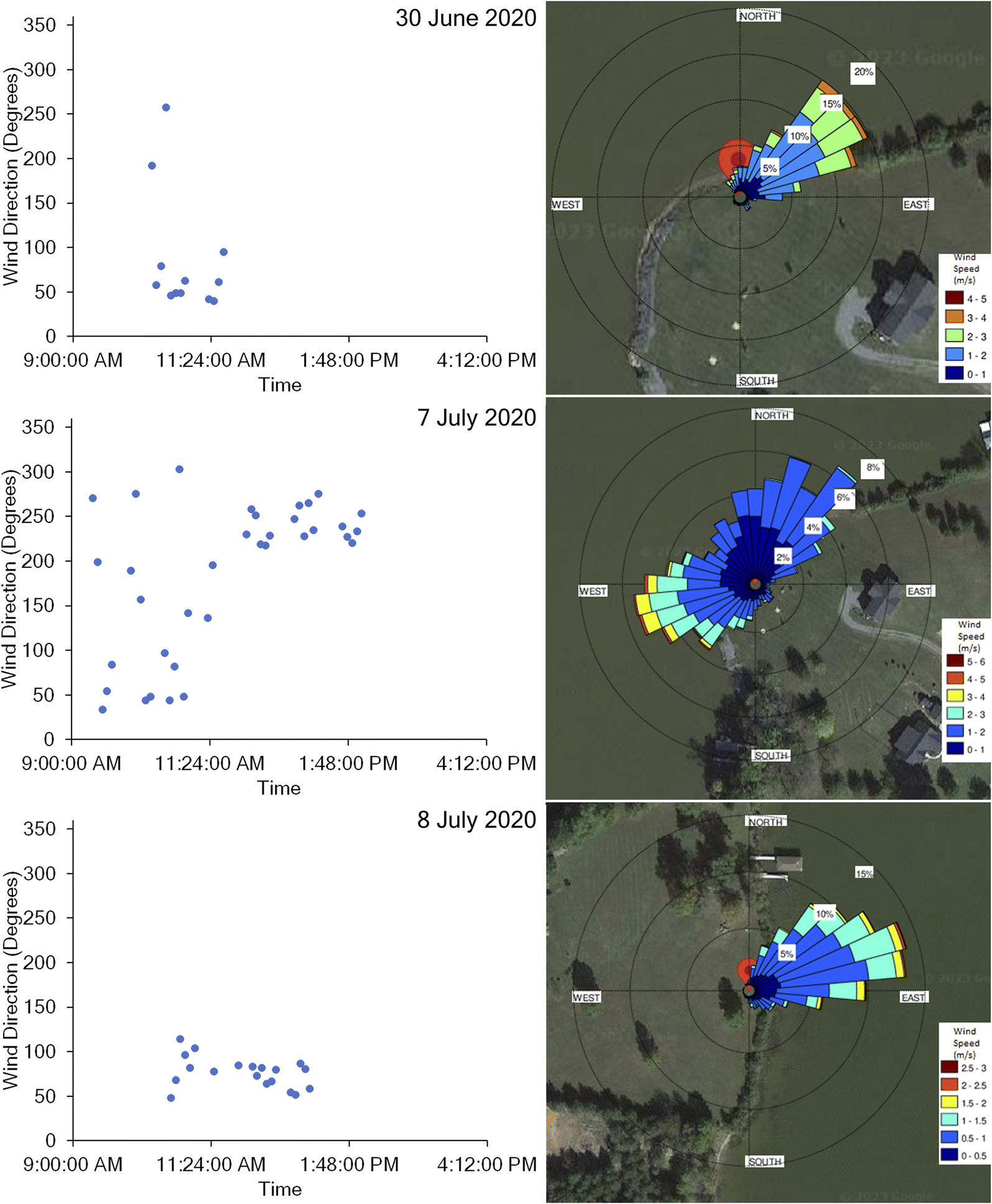
3.1.2 Florida ground-based weather measurements. The wind source direction measured at Seagate beach and Manasota beach in Florida mostly came from the North during our campaign. Easterly morning winds shifted to Northwest winds later in the day (Fig. 6). This trend is more clearly visible at Manasota beach where sampling was started earlier in the day.

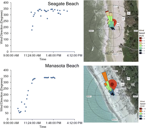Fig. 6 The graphs show wind direction source measured over time at two different Florida beaches in December 2019 plotted as five-minute averages. The top graph shows measurements taken at Seagate beach on December 3rd while the bottom graph shows measurements taken at Manasota beach on December 4th. To the right of each graph is the sensor location with the wind rose for the day.

3.1.3 Supplementary data on reported counts of potentially toxic cyanobacteria in Lake Anna and K. brevis near beach sites in Florida. Counts of potentially toxigenic cyanobacteria in Lake Anna, Virginia in 2019 and 2020 are reported in ESI Tables S1 and S2.† The genus with the largest number of counts in both years was Rhapidioposis, with 8 449 792 and 2 339 584 cell counts recorded in 2019 and 2020, respectively. The relative abundance of the major genera of potentially toxic cyanobacteria in Lake Anna, Virginia are shown in ESI Fig. S1.† Counts of K. brevis in samples collected in December 2019 near Manasota Key and Seagate beaches in Florida are reported in ESI Table S3.† From those samples containing cells of K. brevis, counts ranged from 667 to 8667 reported cells per L for locations near Seagate Beach, and 333 to 8500 reported cells per L for locations near Manasota Key Beach.

3.1.4 Analysis of air and water samples using imaging cytometry. Samples of water (Virginia and Florida) and air (Virginia) contained cells which fluoresced in the red channel (ESI Table S4†), and had morphological similarities to HAB-associated microorganisms (ESI Fig. S3†).

3.2 Particle number concentrations

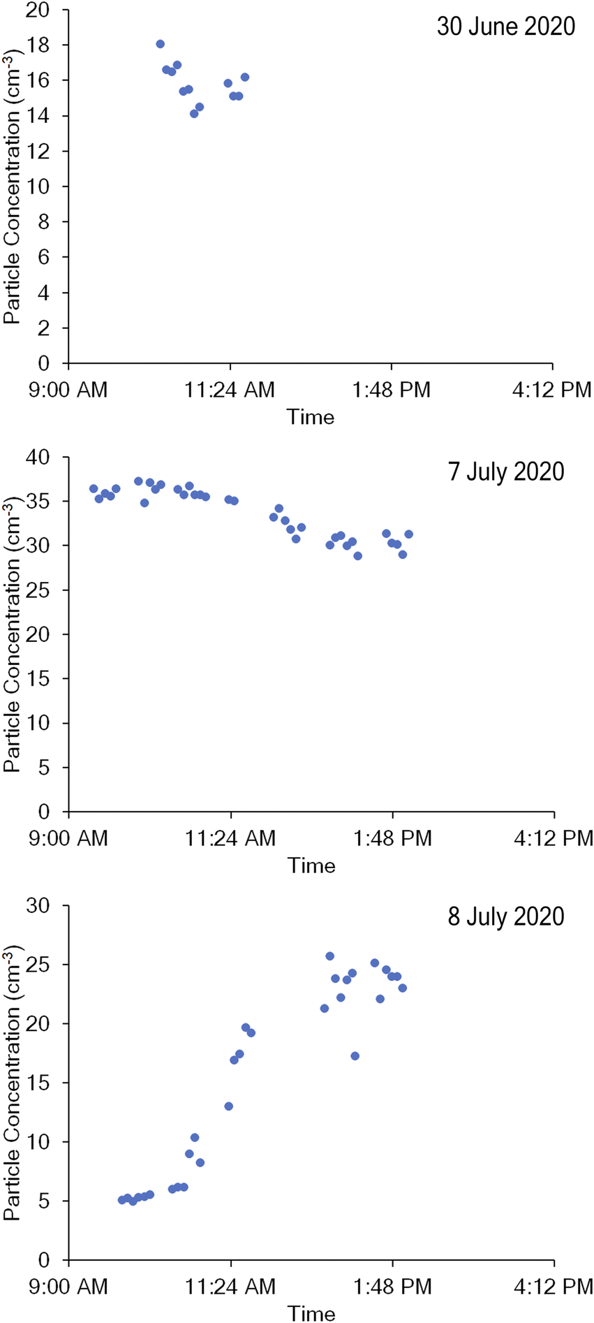
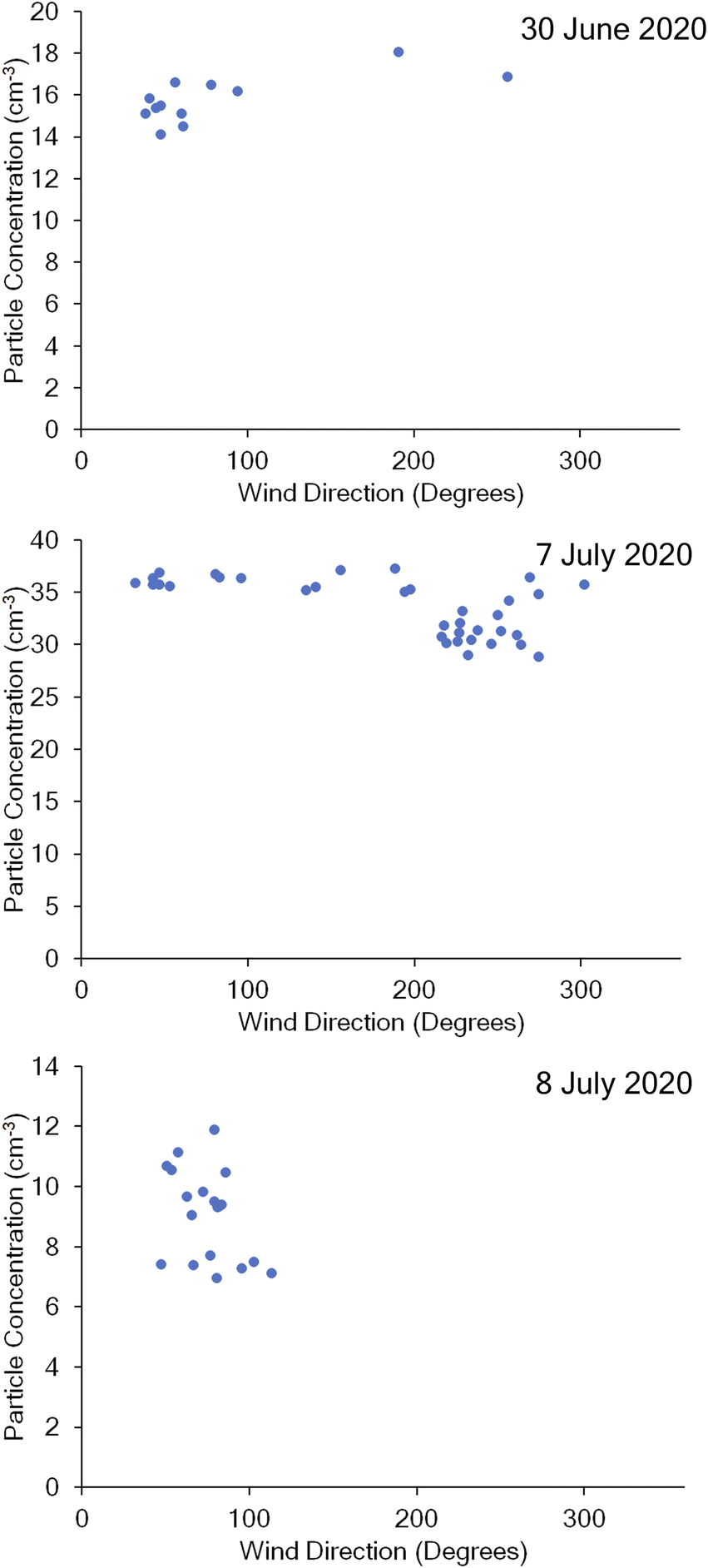
3.2.1 Lake Anna ground-based airborne particle concentrations. Airborne particle concentrations (cm⁻³) at Lake Anna varied over the time of day, and varied over different sampling days, with site 1 showing a decrease in particle number concentrations (cm⁻³) over the course of the sampling periods and site 2 showing an increase in the particle number concentrations (cm⁻³) over the course of the sampling periods (Fig. 7). The particle concentrations at site 1 appeared to be higher on average than those observed at site 2, ranging from 15 to 20 cm⁻³ measured on June 30th and from 25 to 45 cm⁻³ on July 7th, while site 2 had a much lower concentration of particles ranging from 4.5 to 14 cm⁻³. Particle concentrations also showed some correlation with wind source, having lower concentrations for wind sources over land in the July 7th measurements, with wind direction being statistically significant for predicting particle concentration (Fig. 8).

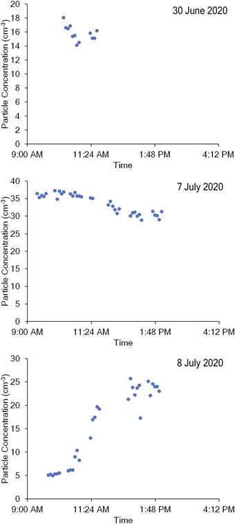Fig. 7 Particle number concentrations (cm⁻³) greater than 0.3 microns in diameter measured over the course of the day, plotted here as five-minute averages. The first two graphs represent June 30th and July 7th at the first Lake Anna shore site and the third graph represents July 8th at the second Lake Anna shore site.

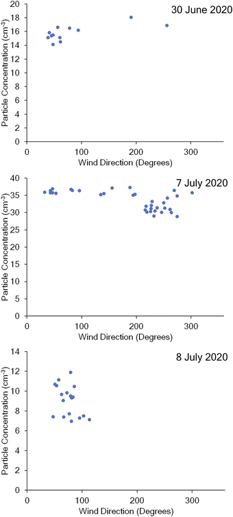Fig. 8 Particle number concentrations (cm⁻³) greater than 0.3 microns in diameter measured wind direction as five-minute averages during the sampling periods at Lake Anna shore sites one and two. The first two graphs depict shore site one during the sampling period of June 30th and July 7th. The third graph shows the data collected from shore site two on July 8th.

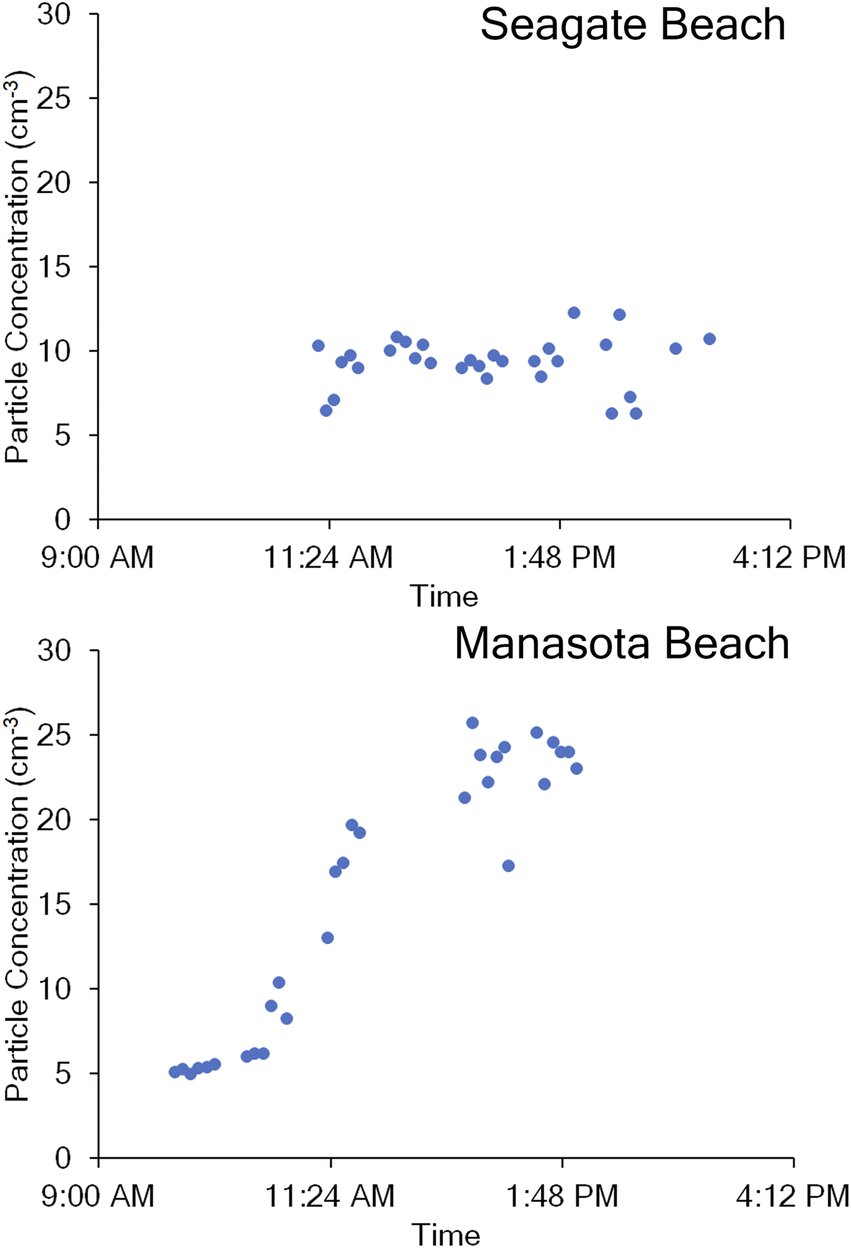
3.2.2 Florida ground-based airborne particle concentrations. Particle number concentrations (cm⁻³) at Seagate beach did not appear to change much over the entire sampling day; however, particle number concentrations (cm⁻³) measured at Manasota beach had a noticeable increase that started during the second sampling period (Fig. 9). Both beaches measured particle number concentrations (cm⁻³) below 5 and highs of above 30 at Seagate beach and above 45 at Manasota beach (Fig. 9). However, while the average particle number concentrations (cm⁻³) at Seagate beach remained low throughout the sampling period, we saw an increase in the particle number concentrations (cm⁻³) at Manasota beach that started in our second sampling period and continued throughout the day.

Fig. 9 The graphs show particle number concentrations (cm⁻³) greater than 0.3 microns in diameter measured over time at two different beaches in Florida on two days in December 2019 plotted as five-minute averages. The top graph shows Seagate beach on December 3rd and the bottom graph shows Manasota beach on December 4th.

3.3 Prediction modeling of particle concentrations due to weather effects

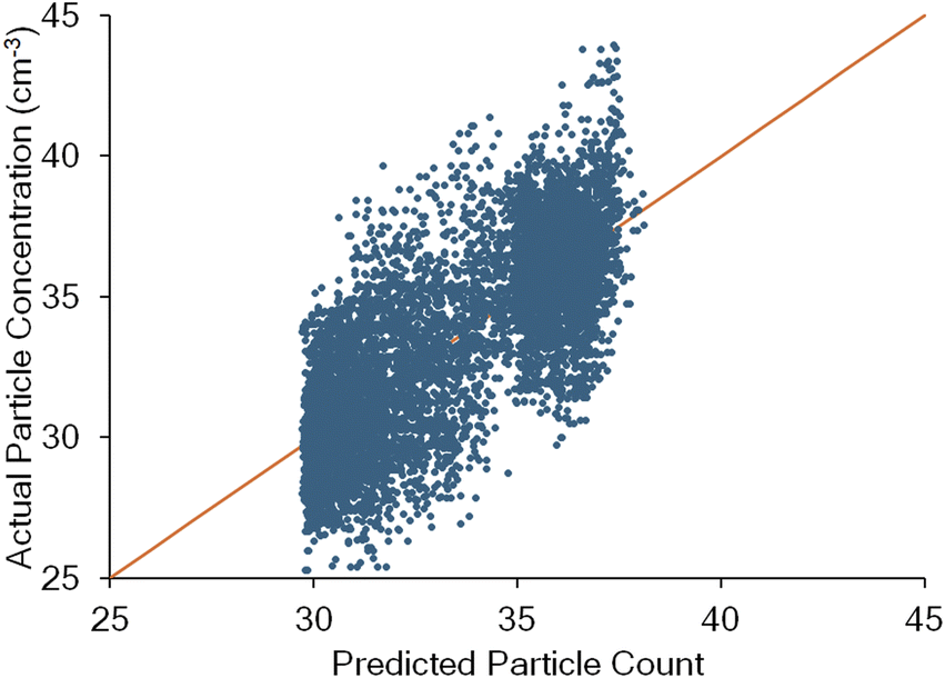
Ground sensor particle number concentrations (cm⁻³) of particles greater than 0.3 μm in diameter were matched with the corresponding weather data collected during the same interval. A prediction equation was developed using the wind speed, wind direction, and temperature data from the collected ground sensor data at Lake Anna on July 7th, 2020, and from Manasota beach on December 4th, 2019, and predicted particle concentrations were compared against the actual measured concentrations (Fig. 10 and 11). The Lake Anna empirical prediction equation produced a model that had an R-squared value of 0.577 and a validation prediction R-squared value of 0.582. The hidden node equations and prediction equation, are as follows:

H₁ = tanh[0.500 (−48.213 + 1.354 WS − 0.014 WD + 1.621T)] (2)

H₂ = tanh[0.500 (26.013 + 0.275 WS − 0.010 WD − 0.789T)] (3)

H₃ = tanh[0.500 (−2.950 + 0.032 WS + 0.0007 WD + 0.153T)] (4)

Theta = 76.18 3 − 316.902H₁ + 640.188H₂ + 4521.478H₃ (5)

where H₁, H₂, and H₃ are the hidden node equations and Theta is the prediction equation giving particle count in number of particles per 0.1 liter as the output. WS is the measured wind speed, WD is the measured wind direction and T is the temperature. The output of the Theta equation is then divided by 100 to get particle count per cubic centimeter.

Fig. 10 Measured vs. predicted particle number concentrations (cm⁻³) of air used in the best fit model for Lake Anna collected data. The model was made using wind speed, wind direction, temperature, and particle count data collected by the ground sensors at Lake Anna. The data was then put into JMP Pro neural network modeling where a model equation was trained on a random subset of the data with another subset held back for validation.

Fig. 11 Measured vs. predicted particle number concentrations (cm⁻³) used in the best fit model for Manasota beach collected data. The model was made using wind speed, wind direction, temperature, and particle count data collected by the ground sensors at Manasota beach. The data was then put into JMP Pro neural network modeling where a model equation was trained on a random subset of the data with another subset held back for validation.

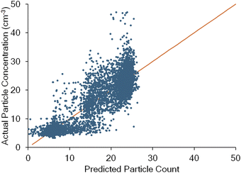
The Manasota beach empirical prediction equation produced a model that had an R-squared value of 0.804 and a validation prediction R-squared value of 0.802. The hidden node equations and prediction equation are as follows:

H₁ = tanh[0.500 (−8.722 − 0.138 WS + 0.024 WD + 0.104T)] (6)

H₂ = tanh[0.500 (38.925 − 1.193 WS − 0.005 WD − 1.693T)] (7)

H₃ = tanh[0.500 (9.500 + 0.154 WS − 0.026 WD − 0.120T)] (8)

Theta = −765.521 − 45377.467H₁ − 682.357H₂ − 43301.880H₃ (9)

where H₁, H₂, and H₃ are the hidden node equations and Theta is the prediction equation giving particle count in number of particles per 0.1 liter as the output. WS is the measured wind speed, WD is the measured wind direction and T is the temperature. The output of the Theta equation is then divided by 100 to get particle count per cubic centimeter.

3.4 Surface flux calculated for beach sites

By using the values collected by the OPC and attached weather sensor, we were able to determine the C_s and V_wind for 30 minute intervals at each beach site. Intervals were divided into onshore or offshore wind sources. The S₁₀₀ was calculated for each 30 minutes interval and the flux from the onshore source wind was subtracted from offshore source wind. On Seagate beach the calculated flux ranged from 522 to 878 cm⁻² s⁻¹ with an average flux of 645 cm⁻² s⁻¹. On Manasota beach, the calculated flux ranged from 940 to 3549 cm⁻² s⁻¹ with an average flux of 2692 cm⁻² s⁻¹.

4. Discussion

Freshwater and marine HABs behave in different ways and produce aerosols under different weather conditions.^39–41 Bubble bursting and wave breaking phenomena contribute to the release of HAB aerosols in lake and ocean systems.^17,42 We used a combination of ground and drone-based sensing to measure wind speed, wind direction, temperature, and airborne particle number concentrations (cm⁻³) on the shores of active HABs in Florida and Virginia. Our measurements are congruent with data reported for potentially toxic cyanobacteria in Lake Anna collected by the Virginia Department of Health, and counts of K. brevis reported for locations near two beach sites in Florida collected by the Mote Marine Laboratory (ESI Tables S1–S3, Fig. S1 and S2†). Though we were unable to formally identify Rhapidiopsis (Lake Anna) and K. brevis (Florida) in our air and water samples using flow cytometry (ESI Table S4 and Fig. S3†), our study provides new information on environmental conditions associated with increased particle number concentrations (cm⁻³) at active HAB sites and could contribute to measurements of potential human exposure to HAB toxins.^4,6,23,43

The particle number concentrations (cm⁻³) measured by a Plantower PMS 7003 OPC were used for comparison only against their own measurements in this study. Previous work with inexpensive OPCs and with the Plantower brand have shown the total particle number concentrations (cm⁻³) increased and decreased in tandem with more expensive and more reliable sensors while the bin sizes were less accurate.^44–46 Our results showed the same inconsistency for the sensor's ability to correctly size particles, so we have chosen to use total measured particle number concentrations (cm⁻³) greater than 0.3 μm diameter. Overall, less expensive OPCs seem to be reliable for measurements showing change in total particle number concentrations (cm⁻³).^46–48 By using the measured total particle number concentrations (cm⁻³), which we compared with our recorded weather conditions of wind speed, wind direction, and temperature, we were able to measure how weather affects total particle count. In a previous study, it was shown that higher particle number concentrations (cm⁻³) are likely associated with HAB aerosols.^21,22

At the Lake Anna sites, airborne particle number concentrations (cm⁻³) decreased over the sampling day at site 1 and increased over the sampling day at site 2. When testing the parameters of the prediction model, the measured wind speed was most strongly associated with higher particle number concentrations (cm⁻³) measured on the shore. When wind directions were coming from offshore, the assumption was that the observed aerosols were produced from offshore sources. It is important to note that we were unable to completely separate the combined effects of higher wind speeds associated with the offshore winds. Additional measurements at higher wind speeds could be collected at both onshore and offshore sources, and these data could help improve our models and add value to future HAB-aerosol risk assessment programs. Previous studies have shown airborne particle concentrations are influenced by windspeed on a lake surface, while shore based measurements have shown decreases in particle number concentrations (cm⁻³) associated with higher wind speeds.^5,24 Studies have shown lake HAB aerosols can contain toxins that may be transported large distances beyond the shore.^49,50 We have previously shown that particle number concentrations (cm⁻³) are significantly influenced by weather effects over the water in lake systems through similar particle and weather monitoring.²² At the Florida sites, airborne particle number concentrations (cm⁻³) increased throughout the day and the wind direction (offshore versus onshore) was strongly associated with these number concentrations (cm⁻³). Offshore wind sources had particle number concentrations (cm⁻³) 3 to 4 times higher than those of onshore wind sources. When developing the prediction equation for the Florida sites, the wind direction had the greatest influence on particle number concentrations (cm⁻³) (P < 0.001), followed by temperature (P < 0.001), and windspeed (P < 0.001). This is consistent with previous studies performed on ocean shores measuring aerosols produced by wave breaking phenomena and their potential to expose the beach to toxins.^7,43,51 Our approach of measuring particle levels at the shore using inexpensive particle counters shows a potential low-cost method for monitoring HAB-associated aerosols on beaches.

A predictive model, trained on a random set of weather and particle count measurements collected over the same time period, was able to predict airborne particle number concentrations (cm⁻³) with an R Squared value of 0.581 for the freshwater HAB in Virginia and an R Squared value of 0.804 for the marine HAB in Florida. Previous methods to monitor HAB severity and inform the public have relied on time-consuming water and aerosol testing or more subjective measurements of respiratory irritation levels.^36,51 We were able to create a prediction equation for a beach and lake site, the conditions that lead to higher levels of particle number concentrations (cm⁻³) in the prediction equations were different in the lake and ocean system and were different between lakes when compared to a previous study.²² For example, the influence of wind speed on the level of particles could be more important for the lake system we measured due to the differences in how aerosols are produced in lake and ocean systems.^4,24,52 In both ocean and lake systems, we were able to predict higher or lower levels of HAB aerosols due to the influence of measured weather conditions. Using this method, any ocean or lake experiencing a HAB could be monitored and set up with a model to predict HAB severity.

Surface flux provides an emission rate for aerosol production at the water surface.⁵³ Using known conditions about wave structure, wind speed, and particle number concentrations (cm⁻³) on shore, the surface flux can be calculated. We were able to calculate the surface flux for the beach sites during our sample period using the equation from Clarke et al.³⁸ This analysis can be performed with ocean occurring HAB sites but there is currently no similar method for lake systems, as the method of aerosolization is different and less well studied.^39,40,54 While our current results show that the better understood ocean aerosol system allows for more robust analysis through surface flux calculations, with more research into lake aerosols we should have better prediction equations available in the future.

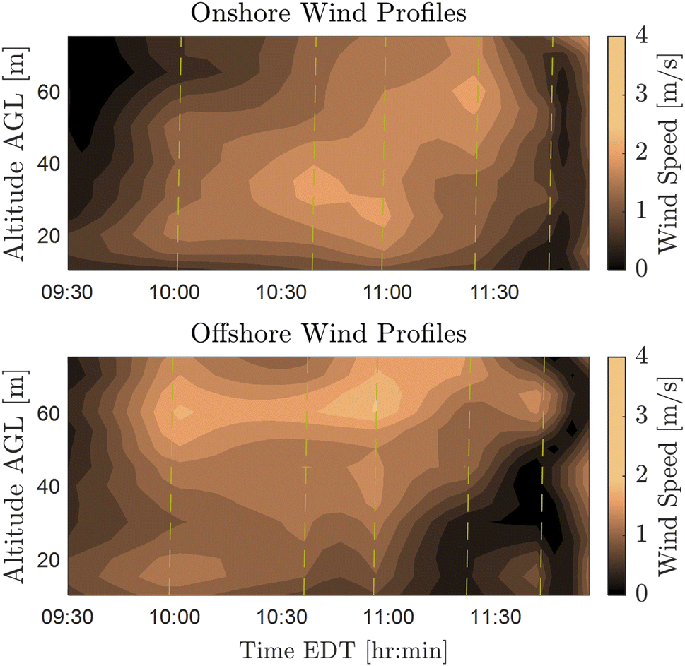
The drone-based vertical profiles of the wind velocity showed differences in wind speed and direction at different altitudes, highlighting the need for wind measurements at multiple heights to capture environmental conditions driving the atmospheric transport of aerosolized HAB toxins. The comparison of onshore and offshore wind speed profiles shows the wind speed to be higher over the water. The higher wind speed conditions observed over water are likely due to the lower roughness length of the lake surface.^39,49 As shown in Fig. 6, the vertical wind speed gradient was also observed to be larger over the lake. The higher wind speed gradient measured over the lake is likely the result of lower surface temperatures. Lower surface temperatures produce less air mixing in the lower atmosphere, resulting in higher wind gradients due to wind shear.^24,55 Furthermore, the comparison of sUAS and ground sensor wind measurements shows that drones can provide reliable observations of wind velocity.^27,31

Higher resolutions of wind velocity observations such as those collected by drone-based measuring platforms are critical for predicting the transport of toxins produced by HABs. Additional work is needed to better understand the short-term fate and transport of aerosolized cyanobacterial cells and toxins and how the local weather conditions influence their transport. Future work might leverage additional chemical (cyanotoxin) or biological (DNA-based) analyses of our water and air samples to help inform these efforts. Risks at the shoreline may not accurately measure the risk of long-range transport that could be driven by higher altitude winds.⁵⁶ Lake aerosols are known to travel long distances and therefore better understanding their downwind fate is important to informing public health surrounding HABs.^17,39 While our current methods of analysis for lake systems are not as accurate as ocean systems, lakes still play an important part in HAB aerosol production and distribution which requires further study.^39,57 This study was focused on the measurements of particles at the shore, but the combined wind measurements at different altitudes may provide insights into yet unexplored areas of HAB aerosol transport. In future studies, combining drone particle count measurements with air and ground wind measurements could help determine not only the near-shore impact of HAB toxins, but also predict their long-term fate. Using these data along with predictive models could then allow for broadcasting air quality as it relates to HABs to inform public safety and use of areas, lake, or ocean, impacted by HABs.

Data availability

Data used in this manuscript are accessible upon request from the corresponding author. Data used in the ESI Tables† are available in public repositories as indicated. There are no restrictions on data access due to privacy or ethical concerns.

Author contributions

LB and RH conducted field experiments for the Florida sites. RH and JGR conducted field experiments for the Lake Anna sites. SR assisted in field experiment site selection in Florida. SR and HF assisted in field experiments in Florida. LB analyzed all ground sensor data from all experiments. JGR analyzed all data from drone measurements. NA and HF implemented the surface flux equation. DS planned experiments at Florida and Lake Anna sites along with LB, RH, and JGR. LB and DS led the writing of the manuscript. KA helped gather and compile the red tide data. All authors provided feedback on the manuscript.

Conflicts of interest

There are no conflicts of interest to declare.

Acknowledgements

This work was supported in part by grants to DS from the U.S. National Science Foundation (NRI-2001119 and IIS-1922516) and the Institute for Critical Technology and Applied Science at Virginia Tech (ICTAS-178429). This work was also supported by a grant to HF, SR, and DS from the Global Change Center and the Institute for Society, Culture, and the Environment at Virginia Tech. The authors thank members of the Lake Anna Civic Association (LACA), including Greg Baker and Harry Looney, for providing access to the Lake Anna sampling locations.

References

1. L. C. Backer, D. Manassaram-Baptiste, R. LePrell and B. Bolton, Cyanobacteria and algae blooms: review of health and environmental data from the harmful algal bloom-related illness surveillance system (HABISS) 2007–2011, Toxins, 2015, 7(4), 1048–1064.
2. S. B. Watson, B. A. Whitton, S. N. Higgins, H. W. Paerl, B. W. Brooks and J. D. Wehr, Chapter 20 – Harmful algal blooms, in Freshwater Algae of North America, ed. J. D. Wehr, R. G. Sheath and J. P. Kociolek, Academic Press, Boston, 2 edn, 2015, pp. 873–920, (Aquatic Ecology). Available from: https://www.sciencedirect.com/science/article/pii/B9780123858764000207.
3. D. G. Schmale, A. P. Ault, W. Saad, D. T. Scott and J. A. Westrick, Perspectives on harmful algal blooms (HABs) and the cyberbiosecurity of freshwater systems, Front. Bioeng. Biotechnol., 2019, 7, 128.
4. J. Hu, J. Liu, Y. Zhu, Z. Diaz-Perez, M. Sheridan and H. Royer, et al., Exposure to aerosolized algal toxins in south florida increases short- and long-term health risk in drosophila model of aging, Toxins, 2020, 12(12), 787.
5. C. W. Powers, R. Hanlon, H. Grothe, A. J. Prussin, L. C. Marr and D. G. Schmale, Coordinated sampling of microorganisms over freshwater and saltwater environments using an unmanned surface vehicle (USV) and a small unmanned aircraft system (sUAS), Front. Microbiol., 2018, 1668.
6. R. H. Pierce, M. S. Henry, P. C. Blum, J. Lyons, Y. S. Cheng and D. Yazzie, et al., Brevetoxin concentrations in marine aerosol: human exposure levels during a karenia brevis harmful algal bloom, Bull. Environ. Contam. Toxicol., 2003, 70(1), 161–165.
7. S. D. Ross, J. Fish, K. Moeltner, E. M. Bollt, L. Bilyeu and T. Fanara, Beach-level 24-hour forecasts of Florida red tide-induced respiratory irritation, Harmful Algae, 2022, 111, 102149.
8. D. M. Anderson, P. M. Glibert and J. M. Burkholder, Harmful algal blooms and eutrophication: nutrient sources, composition, and consequences, Estuaries, 2002, 25(4), 704–726.
9. I. Bertani, D. R. Obenour, C. E. Steger, C. A. Stow, A. D. Gronewold and D. Scavia, Probabilistically assessing the role of nutrient loading in harmful algal bloom formation in western Lake Erie, J. Great Lakes Res., 2016, 42(6), 1184–1192.
10. J. Hoorman, T. Hone, T. Sudman, T. Dirksen, J. Iles and K. R. Islam, Agricultural impacts on lake and stream water quality in grand lake St. Marys, Western Ohio, Water Air Soil Pollut., 2008, 193(1), 309–322.
11. T. J. Smayda, Harmful algal blooms: their ecophysiology and general relevance to phytoplankton blooms in the sea, Limnol. Oceanogr., 1997, 42(5part2), 1137–1153.
12. F. X. Fu, A. O. Tatters and D. A. Hutchins, Global change and the future of harmful algal blooms in the ocean, Mar. Ecol. Prog. Ser., 2012, 470, 207–233.
13. P. Dees, E. Bresnan, A. C. Dale, M. Edwards, D. Johns and B. Mouat, et al., Harmful algal blooms in the Eastern North Atlantic Ocean, Proc. Natl. Acad. Sci. U. S. A., 2017, 114(46), E9763–E9764.
14. M. L. Wells and B. Karlson, Harmful algal blooms in a changing ocean, in Global Ecology and Oceanography of Harmful Algal Blooms, ed. P. M. Glibert, E. Berdalet, M. A. Burford, G. C. Pitcher and M. Zhou, Springer International Publishing, Cham, 2018, pp. 77–90, (Ecological Studies),  DOI:10.1007/978-3-319-70069-4_5.
15. M. L. Wells, B. Karlson, A. Wulff, R. Kudela, C. Trick and V. Asnaghi, et al., Future HAB science: directions and challenges in a changing climate, Harmful Algae, 2020, 91, 101632.
16. B. Kirkpatrick, R. Pierce, Y. S. Cheng, M. S. Henry, P. Blum and S. Osborn, et al., Inland transport of aerosolized Florida red tide toxins, Harmful Algae, 2010, 9(2), 186–189.
17. N. E. Olson, M. E. Cooke, J. H. Shi, J. A. Birbeck, J. A. Westrick and A. P. Ault, Harmful algal bloom toxins in aerosol generated from inland lake water, Environ. Sci. Technol., 2020, 54(8), 4769–4780.
18. R. C. Thakur, L. Dada, L. J. Beck, L. L. J. Quéléver, T. Chan and M. Marbouti, et al., An evaluation of new particle formation events in Helsinki during a Baltic Sea cyanobacterial summer bloom, Atmos. Chem. Phys., 2022, 22(9), 6365–6391.
19. H. E. Plaas, R. W. Paerl, K. Baumann, C. Karl, K. J. Popendorf and M. A. Barnard, et al., Harmful cyanobacterial aerosolization dynamics in the airshed of a eutrophic estuary, Sci. Total Environ., 2022, 852, 158383.
20. T. E. Maloney and R. A. Carnes, Toxicity of a microcystis waterbloom from an ohio pond, Ohio J. Sci., 1966, 66(5), 514–517.
21. L. Bilyeu, B. Bloomfield, R. Hanlon, J. González-Rocha, J. Jacquemin S and P. Ault A, et al., Drone-based particle monitoring above two harmful algal blooms (HABs) in the USA, Environ. Sci. Atmos., 2022, 2(6), 1351–1363.
22. R. Hanlon, S. J. Jacquemin, J. A. Birbeck, J. A. Westrick, C. Harb and H. Gruszewski, et al., Drone-based water sampling and characterization of three freshwater harmful algal blooms in the United States, Front. Remote Sens., 2022, 3, 949052.
23. W. W. Carmichael and G. L. Boyer, Health impacts from cyanobacteria harmful algae blooms: implications for the North American Great Lakes, Harmful Algae, 2016, 54, 194–212.
24. M. E. Dueker, G. D. O'Mullan, J. M. Martínez, A. R. Juhl and K. C. Weathers, Onshore wind speed modulates microbial aerosols along an urban waterfront, Atmosphere, 2017, 8(11), 215.
25. K. Moeltner, T. Fanara, H. Foroutan, R. Hanlon, V. Lovko and S. Ross, et al., Harmful algal blooms and toxic air: the economic value of improved forecasts, Mar. Resour. Econ, 2023, 38(1), 1–28.
26. J. González-Rocha, S. F. J. De Wekker, S. D. Ross and C. A. Woolsey, Wind profiling in the lower atmosphere from wind-induced perturbations to multirotor UAS, Sensors, 2020, 20(5), 1341.
27. J. González-Rocha, L. Bilyeu, D. Ross S, H. Foroutan, J. Jacquemin S and P. Ault A, et al., Sensing atmospheric flows in aquatic environments using a multirotor small uncrewed aircraft system (sUAS), Environ. Sci. Atmos., 2023, 3(2), 305–315.
28. T. F. Villa, F. Gonzalez, B. Miljievic, Z. D. Ristovski and L. Morawska, An overview of small unmanned aerial vehicles for air quality measurements: present applications and future prospectives, Sensors, 2016, 16(7), 1072.
29. A. Samad, D. Alvarez Florez, I. Chourdakis and U. Vogt, Concept of using an unmanned aerial vehicle (UAV) for 3D investigation of air quality in the atmosphere—example of measurements near a roadside, Atmosphere, 2022, 13(5), 663.
30. D. Wu, R. Li, F. Zhang and J. Liu, A review on drone-based harmful algae blooms monitoring, Environ. Monit. Assess., 2019, 191, 1–11.
31. J. González-Rocha, C. A. Woolsey, C. Sultan and S. F. J. De Wekker, Sensing wind from quadrotor motion, J. Guid. Control Dyn., 2019, 42(4), 836–852.
32. C. Harb and H. Foroutan, A systematic analysis of the salinity effect on air bubbles evolution: laboratory experiments in a breaking wave analog, J. Geophys. Resour. Oceans, 2019, 124(11), 7355–7374.
33. C. Harb, J. Pan, S. DeVilbiss, B. Badgley, L. C. Marr and D. G. Schmale, et al., Increasing freshwater salinity impacts aerosolized bacteria, Environ. Sci. Technol., 2021, 55(9), 5731–5741.
34. R. P. Stumpf, Applications of satellite ocean color sensors for monitoring and predicting harmful algal blooms, Hum. Ecol. Risk Assess. Int. J., 2001, 7(5), 1363–1368.
35. Lake Anna State Park, General information, 2023. Available from: https://www.dcr.virginia.gov/state-parks/lake-anna#general_information.
36. Mote Beach Conditions Reporting System, 2022, Available from: https://visitbeaches.org/map.
37. E. Morelli and V. Klein, Aircraft System Identification: Theory and Practice, Sunflyte Enterprises, Williamsburg, VA, 2016, vol. 2, pp. 77–79.
38. A. D. Clarke, S. R. Owens and J. Zhou, An ultrafine sea-salt flux from breaking waves: implications for cloud condensation nuclei in the remote marine atmosphere, J. Geophys. Res. Atmos., 2006, 111(D6), D06202.
39. N. W. May, J. L. Axson, A. Watson, K. A. Pratt and A. P. Ault, Lake spray aerosol generation: a method for producing representative particles from freshwater wave breaking, Atmos. Meas. Technol. Discuss., 2016, 4311–4325.
40. N. W. May, M. J. Gunsch, N. E. Olson, A. L. Bondy, R. M. Kirpes and S. B. Bertman, et al., Unexpected contributions of sea spray and lake spray aerosol to inland particulate matter, Environ. Sci. Technol. Lett., 2018, 5(7), 405–412.
41. P. Li, L. Li, K. Yang, T. Zheng, J. Liu and Y. Wang, Characteristics of microbial aerosol particles dispersed downwind from rural sanitation facilities: Size distribution, source tracking and exposure risk, Environ. Res., 2021, 195, 110798.
42. G. B. Deane and M. D. Stokes, Scale dependence of bubble creation mechanisms in breaking waves, Nature, 2002, 418(6900), 839–844.
43. R. H. Pierce, M. S. Henry, P. C. Blum, S. L. Hamel, B. Kirkpatrick and Y. S. Cheng, et al., Brevetoxin composition in water and marine aerosol along a Florida beach: assessing potential human exposure to marine biotoxins, Harmful Algae, 2005, 4(6), 965–972.
44. Z. M. Levy, F. Xiong, D. Gentner, B. Kerkez, J. Kohrman-Glaser and K. Koehler, Field and laboratory evaluations of the low-cost plantower particulate matter sensor, Environ. Sci. Technol., 2019, 53(2), 838–849.
45. D. H. Hagan and J. H. Kroll, Assessing the accuracy of low-cost optical particle sensors using a physics-based approach, Atmos. Meas. Technol., 2020, 13(11), 6343–6355.
46. M. He, N. Kuerbanjiang and S. Dhaniyala, Performance characteristics of the low-cost plantower PMS optical sensor, Aerosol. Sci. Technol., 2020, 54(2), 232–241.
47. N. Sang-Nourpour and J. S. Olfert, Calibration of optical particle counters with an aerodynamic aerosol classifier, J. Aerosol. Sci., 2019, 138, 105452.
48. L. R. Crilley, A. Singh, L. J. Kramer, M. D. Shaw, M. S. Alam and J. S. Apte, et al., Effect of aerosol composition on the performance of low-cost optical particle counter correction factors, Atmos. Meas. Technol., 2020, 13(3), 1181–1193.
49. N. W. May, N. E. Olson, M. Panas, J. L. Axson, P. S. Tirella and R. M. Kirpes, et al., Aerosol emissions from great lakes harmful algal blooms, Environ. Sci. Technol., 2018, 52(2), 397–405.
50. J. Sutherland, The detection of airborne anatoxin-a (ATX) on glass fiber filters during a harmful algal bloom, Lake Reservoir Manage., 2021, 37(2), 113–119.
51. B. Kirkpatrick, L. E. Fleming, J. A. Bean, K. Nierenberg, L. C. Backer and Y. S. Cheng, et al., Aerosolized red tide toxins (brevetoxins) and asthma: continued health effects after 1h beach exposure, Harmful Algae, 2011, 10(2), 138–143.
52. N. E. Olson, M. E. Cooke, J. H. Shi, J. A. Birbeck, J. A. Westrick and A. P. Ault, Harmful algal bloom toxins in aerosol generated from inland lake water, Environ. Sci. Technol., 2020, 54(8), 4769–4780.
53. N. Meskhidze, M. D. Petters, K. Tsigaridis, T. Bates, C. O'Dowd and J. Reid, et al., Production mechanisms, number concentration, size distribution, chemical composition, and optical properties of sea spray aerosols, Atmos. Sci. Lett., 2013, 14(4), 207–213.
54. J. H. Slade, T. M. VanReken, G. R. Mwaniki, S. Bertman, B. Stirm and P. B. Shepson, Aerosol production from the surface of the Great Lakes, Geophys. Res. Lett., 2010, 37(18), L18807.
55. N. I. Medina-Pérez, M. Dall'Osto, S. Decesari, M. Paglione, E. Moyano and E. Berdalet, Aerosol toxins emitted by harmful algal blooms susceptible to complex air–sea interactions, Environ. Sci. Technol., 2021, 55(1), 468–477.
56. S. S. Prijith, M. Aloysius, M. Mohan, N. Beegum and K. Krishna Moorthy, Role of circulation parameters in long range aerosol transport: evidence from winter-ICARB, J. Atmos. Sol.-Terr. Phys., 2012, 77, 144–151.
57. C. Harb and H. Foroutan, Experimental development of a lake spray source function and its model implementation for Great Lakes surface emissions, Atmos. Chem. Phys., 2022, 22(17), 11759–11779.

---

Footnote

† Electronic supplementary information (ESI) available. See DOI: https://doi.org/10.1039/d4va00172a

---