 Open Access Article
An ensemble variable selection method for vibrational spectroscopic data analysis†
Jixiong Zhang a,
Hong Yana,
Yanmei Xionga,
Qianqian Li
 b and
Shungeng Min*a
aCollege of Science, China Agricultural University, No. 2, Yuanmingyuanxi Road, Haidian District, Beijing 100193, P.R. China. E-mail: minsg@cau.edu.cn; Tel: +86-010-62733091
bSchool of Marine Science, China University of Geosciences in Beijing, Beijing 100086, China
First published on 26th February 2019
Abstract
Wavelength selection is a critical factor for pattern recognition of vibrational spectroscopic data. Not only does it alleviate the effect of dimensionality on an algorithm's generalization performance, but it also enhances the understanding and interpretability of multivariate classification models. In this study, a novel partial least squares discriminant analysis (PLSDA)-based wavelength selection algorithm, termed ensemble of bootstrapping space shrinkage (EBSS), has been devised for vibrational spectroscopic data analysis. In the algorithm, a set of subsets are generated from a data set using random sampling. For an individual subset, a feature space is determined by maximizing the expected 10-fold cross-validation accuracy with a weighted bootstrap sampling strategy. Then an ensemble strategy and a sequential forward selection method are applied to the feature spaces to select characteristic variables. Experimental results obtained from analysis of real vibrational spectroscopic data sets demonstrate that the ensemble wavelength selection algorithm can reserve stable and informative variables for the final modeling and improve predictive ability for multivariate classification models.
1. Introduction
Vibrational spectroscopic methods in combination with pattern recognition techniques have been widely exploited in different application domains including food science,1 petrochemicals2 and pharmaceuticals.3,4 A sample is generally characterized with hundreds or even thousands of wavelength variables and some of the variables may contain irrelevant and/or redundant information for classification modeling. To deal with spectroscopic data sets that have a large number of wavelength variables, selection of a smaller number of informative features is important to reduce the problem of dimensionality so that the performance of the models can be increased for interpretative purposes.5,6 This feature selection can be achieved by either replacing the original data domain by a smaller one or by selecting only the most important variables in the original domain.As one of the most popular recognition techniques in chemometrics, partial least squares discriminant analysis (PLS-DA) provides a solution to the problem of irrelevant and redundant inputs.7 The PLD-DA method is a projection-based tool which in principle should ignore the variables space spanned by irrelevant or noisy variables. However, excessive variables and small objects can spoil the PLS-DA results, because PLS-DA has trouble in searching the proper size of variable subspace in high dimensional data.8,9 To data, much effort has been made to improve the performance of PLS-DA, and variable selection has been shown to be one of the most effective ways because there is a close connection between PLS dimension reduction and variable selection.10
A number of algorithms for variable selection in the PLS-DA model have been proposed.5,11–22 In general, these methods can be classified into three categories and include filter, wrapper and embedded techniques.23 Wrapper is the most commonly used technique, because this technique is easy to implement and the interaction between the feature subset search and the classifier is considered. In wrapper methods, a search procedure in the space of the possible feature subset is defined and various subsets of features are generated and evaluated. The evaluation of a specific subset of features is obtained by a PLS-DA model. Examples of such methods are backward variable elimination PLS-DA,21 moving window PLS-DA22 and artificial intelligent algorithm based PLS-DA.6,16,17,19 Recently a bootstrapping strategy coupled with model population analysis was used to search for an optimal variable subset in PLS regression models.24 In this algorithm, various variable subspaces are generated by the weighted bootstrap sampling (WBS) method. Variables with larger absolute values of PLS regression coefficients are extracted and given a higher sampled weight using model population analysis. Whole variable space shrinks gradually until it becomes an optimal variable subset. A similar approach was also used in a study on spectral interval combination optimization.25
In the case of the wrapper variable selection methods guided by a random search, however, a common problem is that they have a high risk of randomicity,26 given that the probability of finding a suitable model may sometimes happen by chance (due to random correlations). Clearly, the stability and reliability of selected results needs to should be strengthened.27
In several notable papers that are concerned with ensemble methods in machine learning,28–31 a set of classifiers whose individual decisions are combined in some way (typically by weighted or unweighted voting) has been shown to provide improved classification accuracy. Inspired by this, we have made the assumption that an ensemble of variable selection methods may be used to extract the most informative and significant variables and to reduce the stochastic risk. In fact, there have been some reports on the use of ensemble methods for variable selection in chemometrics. For instance, Han et al.32 developed a method using an ensemble of Monte Carlo uninformative variable elimination to improve the stability and reliability of selected variables, and Zheng et al.26 used an improved version of a voting genetic algorithm (GA) to overcome the stochastic risk of a GA.
In this study, a new PLSDA-based wavelength selection algorithm, termed ensemble of bootstrapping space shrinkage (EBSS), is proposed to select stable feature variables for pattern recognition of vibrational spectroscopic data. First, some theoretical background for EBSS is introduced (Section 2). Then, to demonstrate the effectiveness of EBSS, the proposed algorithm was applied to four publicly available vibrational spectroscopic datasets (Section 3). The results of EBSS were compared with those obtained from single bootstrapping space shrinkage (BSS), GA-PLS-DA and sparse-PLS-DA (s-PLS-DA) (Section 4). Concluding remarks are given in Section 5.
2. Theory
2.1 PLS-DA
The theory and properties of the PLS-DA have been described elsewhere,33,34 hence only a short overview of the PLS-DA method, which is based on the PLS2 algorithm, is given here. Usually, the PLS-DA model is formulated as a regression equation:| Y = XB | (1) |
 | (2) |
Once the regression coefficients B are obtained, the prediction of dependent variables on a new set of objects can be done by
| Ytest = XtestB | (3) |
However, the predicted values are real numbers and a conversion to class memberships is needed. In this study, the class membership of each unknown sample is assigned as the column index of the largest absolute value in the corresponding row of the Ytest matrix.5
2.2 BSS
The BSS is a basic predictor of EBSS, and it is also a modified version of BOSS.24 The BSS procedure can be summarized in the following steps:For an independent variables space X with size N × P (contains N samples, P variables).
Step 1: the weighted bootstrap sampling (WBS) method24 is applied to the whole variable space to generate M (e.g., 1000) variable subspaces. In each variables subspace, the repeated variables are excluded to remain unique. Note that the initial number of replacements in WBS is equal to P, and the initial sampling weight of each variable is set to 1/P. According to the bootstrap theory, the number of selected variables in each subset is about 0.632P.
Step 2: individual variable subspace is evaluated to determine its accuracy value using a PLS-DA algorithm and 10-fold cross validation is performed for extraction of the best variable subspaces (10%) with the highest accuracy.
Step 3: the appearance frequency of each variable in the best variable subspaces is counted and the sampling weight of variable p can then be updated as follows:
 | (4) |
Step 4: the number of replacements in WBS is updated and the value is determined by the average number of variables selected in the previous step. According to bootstrap theory, the number of variables in a new subset is about 0.632 times the previous one. Thus, variable space shrinks step by step.
Step 5: steps 1–4 are repeated until the average number of variables in the new subspaces equals the number of selected latent variables. The subspace with the best accuracy during the iteration is selected as the optimal variable set.
2.3 EBSS
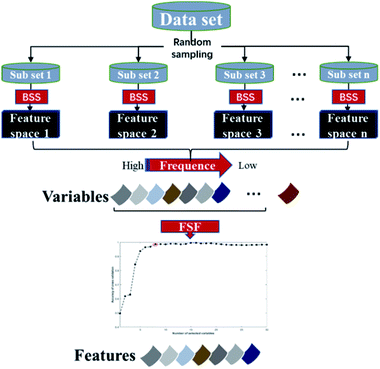
The core idea of the EBSS algorithm is illustrated in Fig. 1. First, a set of subsets are generated from data set using random sampling. For an individual subset, a feature space is determined by BSS. Then an ensemble strategy and a sequential forward selection method are applied to the candidate feature spaces to select characteristic variables. The EBSS procedure can be summarized by the following steps:Step 1: the data set is divided randomly into a training set T and a validation set V. T consists of 67% of the data with V being the remainder. A feature space F is selected from T using the BSS method.
Step 2: repeat step K times to give feature spaces F1, …, FK.
Step 3: extract R the most common recurring variables from the K feature spaces based on eqn (4) (Section 2.2).
Step 4: the final discriminant feature space Fd is determined by running PLS-DA on training sets using from 1 to R of the most recurring variables and 10-fold cross-validation.
Step 5: a PLS-DA is constructed from Ti using Fd. Running the validation set Vi down this PLS-DA gives an accuracy rate ai (Fd, Vi), where i = 1, …, K. The average accuracy rate aave (Fd) and standard error astd (Fd) over the K repeats are computed and recorded.
In this study, K is set to 20, R is set to 30 (for Raman data, R is set to 60).
2.4 Overview of the compared methods
| Population size | 50 chromosomes |
| Maximum number of generations | 100 |
| Generation gap | 0.95 |
| Crossover rate | 0.75 |
| Mutation rate | 0.01 |
| Maximum number of variables selected in the chromosome | 50 |
| Fitness value | accuracy of 10-fold cross-validation of PLSDA |
2.5 Algorithm evaluation
The EBSS algorithm was evaluated by the procedure as described in Section 2.3. For BSS, GA-PLS-DA and s-PLS-DA, each algorithm was evaluated, independently, in the following way:Step 1: the data set was randomly divided into a training set T and a validation set V. T consisted of 67% of the data, and V the remainder.
Step 2: a feature space F was selected from T using the variable selection method. A PLS-DA model was constructed from T using F. Running the validation set V down this PLS-DA gave the accuracy rate a (F, V).
Step 3: steps 1 and 2 were repeated 20 times giving feature spaces F1, …, F20 and accuracy rates a1 (F1, V1), …, a20 (F20, V20). The average accuracy rate aave and the standard error astd over the 20 repeat were computed and recorded.
For all of the algorithms the optimal number of latent variables for PLS-DA model was determined by 10-fold cross-validation, the data set was mean-centered before modeling.16
3. Data sets and experimental condition
3.1 Data sets
![[thin space (1/6-em)]](https://www.rsc.org/images/entities/char_2009.gif) 000 cm−1, Altogether there were 310 samples. Raman spectra were collected in the range 200–3600 cm−1. Altogether there were 120 samples.
000 cm−1, Altogether there were 310 samples. Raman spectra were collected in the range 200–3600 cm−1. Altogether there were 120 samples.An overview of the characteristics of the different data sets is given in Table 2. For each data set, 67% of samples were randomly selected for the training set and those remaining were used as a validation set.24
| Data set | Scan | No. of training samples | No. of test samples | No. of features | No. of classes |
|---|---|---|---|---|---|
| Olive oils | FTIR | 82 | 38 | 570 | 4 |
| Red wines | FTIR | 30 | 14 | 842 | 4 |
| NIR tablets | NIR | 211 | 99 | 404 | 4 |
| Raman tablets | Raman | 82 | 38 | 3401 | 4 |
3.2 Experimental conditions
All computations were performed in MATLAB (Version 2016a, MathWorks, Inc.) on a personal computer (Intel Core i7-7700 3.6 GHz CPU and 8 GB RAM). MATLAB codes for s-PLS-DA were acquired courtesy of Ewa Szymanska. The GA-PLS-DA, BSS and EBSS algorithms were realized with home-made codes which are available upon request.4. Results and discussion
Table 3 gives the validation set accuracies for the different methods. The data in bold denote the best performance on each data set.As Table 3 shows, EBSS gives the best performance relative to the other methods for all datasets. The number of selected variables for each method is given in Table 4. It can be seen that the EBSS method used fewer variables than the other methods.
| Data set | Type | PLS-DA | BSS | GA-PLS-DA | s-PLS-DA | EBSS |
|---|---|---|---|---|---|---|
| a aave ± astd: average accuracy rate ± standard error over 20 repeats. | ||||||
| Olive oil | FTIR | 93.2 ± 2.2 | 94.7 ± 2.6 | 93.6 ± 3.1 | 95.1 ± 3.1 | 96.6 ± 3.2 |
| Red wine | FTIR | 59.3 ± 14.3 | 60 ± 13.4 | 60.4 ± 9.4 | 66.8 ± 9.6 | 71.1 ± 10.2 |
| NIR tablet | NIR | 88.9 ± 2.5 | 87 ± 3.6 | 86.4 ± 3.4 | 88.3 ± 2.9 | 89.3 ± 3.2 |
| Raman tablet | Raman | 85.8 ± 5.7 | 81.4 ± 4.2 | 80.4 ± 4.7 | 78.8 ± 4.9 | 89.3 ± 5.1 |
| Data set | Type | PLS-DA | BSS | GA-PLS-DA | s-PLS-DA | EBSS |
|---|---|---|---|---|---|---|
| a nave ± nstd: average number of selected variable ± standard error over 20 repeats. | ||||||
| Olive oil | FTIR | 570 | 34 ± 33 | 29 ± 10 | 69 ± 22 | 8 |
| Red wine | FTIR | 842 | 43 ± 34 | 33 ± 15 | 52 ± 31 | 21 |
| NIR tablet | NIR | 404 | 46 ± 21 | 44 ± 8 | 59 ± 18 | 20 |
| Raman tablet | Raman | 3041 | 58 ± 22 | 60 ± 8 | 77 ± 19 | 40 |
4.1 Olive oil data set
For the olive oil data set, the accuracy was improved from 93.2% in the case of PLS-DA to 96.6% for the EBSS method. Other variable selection methods also show better classification performance than the full range PLS-DA (BSS: 94.7%, GA-PLS-DA: 93.6%, s-PLS-DA: 95.1%), which demonstrates the benefit of conducting variable selection.The selected wavenumber variables are displayed in Fig. 2. In each subgraph the x-axis represents the wavenumber variables and the y-axis represents the frequency of each variable selected by the algorithm after 20 repeat operations. Instability of the selected sets of informative variables can be found when using BSS and GA-PLA-DA given that these selection methods are guided by a random search. The stability of variable selection performed with s-PLS-DA was better than those for BSS and GA-PLS-DA. For EBSS, eight variables were selected to discriminate between four classes. The eight wavenumbers were 966.8, 1003.4, 1123.1, 1125.0, 1126.9, 1194.1, 1628.6 and 1665.3 cm−1 (see Fig. 2d).
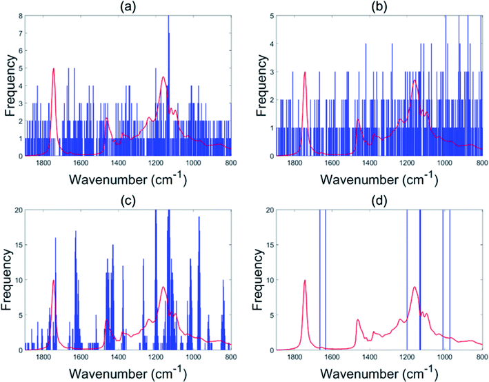 | ||
| Fig. 2 Variables selected by the different methods for the olive oil data: BSS (a), GA-PLS-DA (b), s-PLS-DA (c) and EBSS (d). | ||
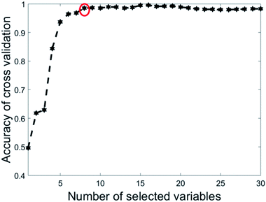
The eight wavenumbers were determined by running PLS-DA using 1 to 30 as the most recurring variables (see Section 2.3). In each iteration, 67% of the data was split off as a training set. Then nVAR, the number of variables selected was varied from 1 to 30. For each value of nVAR, a PLS-DA model was constructed on the training set using 10-fold cross-validation and then the accuracy of cross-validation was recorded. Twenty iterations were done, and the accuracy values were averaged over 20 repetitions. Fig. 3 is a plot of the accuracy of cross-validation vs. nVAR. The result is fascinating. The cross-validation accuracy increases from nVAR = 1 to nVAR = 8. Beyond about nVAR = 8 the accuracy remained constant, i.e., adding more variables did not improve accuracy.
4.2 Red wine data set
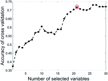
This data set had only 44 as the total number of samples with BSS giving a validation set accuracy of 60% and GA-PLS-DA had an accuracy of 60.4%. The s-PLS-DA had an accuracy of 66.8%, which was a 12.6% improvement compared with 59.3% using full range PLS-DA. The EBSS method gave an accuracy of 71.1%, an improvement of 19.9%. These results illustrate that variable selection is necessary to improve the separation ability, and that PLS-DA may not be a good choice for small samples datasets.39Fig. 4 shows the selected variables for the different methods. The BSS, GA-PLS-DA and s-PLS-DA methods produced different feature spaces in each repeat. In total, 21 wavenumber variables were selected by EBSS. The selected variables are also listed in the Appendix (Table 5). The way that was used to reserve the 21 variables was the same as that for the olive oil dataset. Fig. 5 is a plot of the accuracy of cross-validation vs. nVAR. The accuracy values increased from nVAR = 1 to nVAR = 10, a small drop occurred from nVAR = 11 to nVAR = 14, then the accuracy gradually increased and remained constant beyond about nVAR = 21.
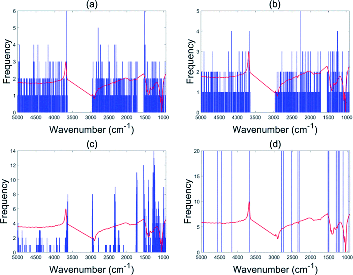 | ||
| Fig. 4 Variables selected by the different methods for the red wine data set: BSS (a), GA-PLS-DA (b), s-PLS-DA (c) and EBSS (d). | ||
4.3 Tablet data sets
The EBSS method gave better performance than full range PLS-DA for both the NIR and Raman tablet data sets. For the NIR tablet data set, the EBSS model had an 89.3% validation accuracy based on only 20 selected variables (Fig. 6d). For the Raman tablet data set, the EBSS model was found to have an 89.3% validation accuracy and the total number of selected variables was 40 (Fig. 7d). From Fig. 6 and 7, it can also be observed that the wavelengths selected by BSS, GA-PLS-DA and s-PLS-DA for the NIR and Raman data sets were labile.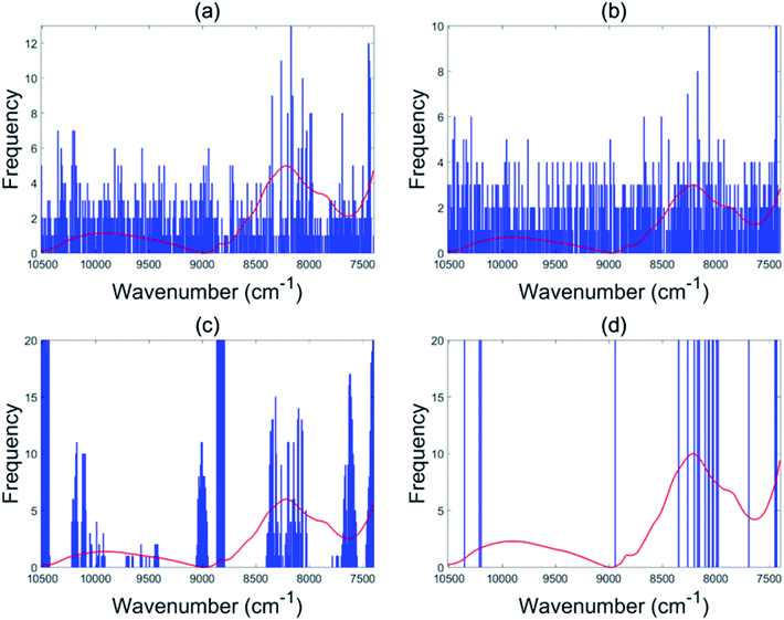 | ||
| Fig. 6 Variables selected by the different methods for the NIR tablet data: BSS (a), GA-PLS-DA (b), s-PLS-DA (c) and EBSS (d). | ||
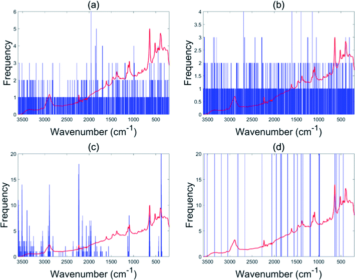 | ||
| Fig. 7 Variables selected by the different methods for the Raman tablet data: BSS (a), GA-PLS-DA (b), s-PLS-DA (c) and EBSS (d). | ||
Fig. 8 shows the effect of the number of selected variables on the accuracy of cross-validation. For the NIR tablet data, the accuracies steadily increased from nVAR = 1 to nVAR (e.g., about 20), and then remained constant (see Fig. 8a). For the Raman tablet data, the number of selected variables was varied from 1 to 60. Again, the accuracies showed a steady increase from nVAR = 1 to nVAR = 40, and then remained constant (see Fig. 8b).
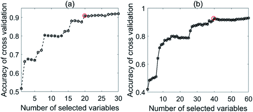 | ||
| Fig. 8 Effect of selected variables on the accuracy for the tablet data sets: (a) NIR and (b) Raman. | ||
As the above results demonstrated, the EBSS method was superior to GA-PLS-DA, BSS and s-PLS-DA in terms of performance.
5. Conclusion
A method termed EBSS, which feature contains bootstrap sampling and an ensemble strategy, has been proposed to select characteristic variables for pattern recognition of vibrational spectroscopic data. The results suggest that the new EBSS algorithm can reserve more stable and informative variables for the final modeling and provide better performance than those obtained from GA-PLS-DA, BSS and s-PLS-DA.The investigations also suggest that EBSS can be an alternative method for rapid classification problem solving with IR, NIR and Raman spectroscopic data. There are many important potential application areas for the EBSS method, such as in biotechnology, food science and medicine, where there is an increasing interest in using atomic and molecular spectroscopies for rapid screening purposes. A challenge is to identify a stable and small number of wavelengths and incorporate into low-cost and accurate instruments tailored to solving specific screening problems.
Appendix
| Data set | Wavenumber (cm−1) |
|---|---|
| Olive oil | 966.8, 1003.4, 1123.1, 1125.0, 1126.9, 1194.1, 1628.6, 1665.3 |
| Red wine | 956.0, 1114.1, 1202.8, 1222.0, 1237.5, 1279.9, 1303.0, 1499.6, 1518.9, 1526.6, 2313.0, 2347.7, 2525.0, 2733.2, 2737.1, 2798.7, 3666.1, 4167.3, 4444.8, 4556.6, 4919.0 |
| Tablet (NIR) | 7429.2, 7436.9, 7444.6, 7691.5, 7976.9, 7992.4, 8023.2, 8030.9, 8061.8, 8069.5, 8100.4, 8154.4, 8169.8, 8200.6, 8347.2, 8941.2, 10![[thin space (1/6-em)]](https://www.rsc.org/images/entities/char_2009.gif) 198.7, 10 198.7, 10![[thin space (1/6-em)]](https://www.rsc.org/images/entities/char_2009.gif) 214.1, 10 214.1, 10![[thin space (1/6-em)]](https://www.rsc.org/images/entities/char_2009.gif) 353.0 353.0 |
| Tablet (Raman) | 3575, 3514, 3345, 3192, 3048, 3047, 2826, 2816, 2666, 2279, 2058, 2056, 1957, 1955, 1954, 1858, 1840, 1839, 1838, 1703, 1701, 1699, 1556, 1477, 1356, 1395, 1196, 1194, 1193, 1191, 1190, 993, 989, 983, 982, 639, 632, 597, 540, 449 |
Conflicts of interest
There are no conflicts to declare.Acknowledgements
The authors would like to thank Ewa Szymanska, from Radboud University Nijmegen, The Netherlands for providing the sparse-PLS-DA codes. We also grateful to Kuangda Tian for providing helpful suggestions for our research.References
- H. S. Tapp, A. Marianne Defernez and E. K. Kemsley, J. Agric. Food Chem., 2003, 51, 6110–6115 CrossRef CAS PubMed.
- R. M. Balabin, R. Z. Safieva and E. I. Lomakina, Anal. Chim. Acta, 2010, 671, 27–35 CrossRef CAS PubMed.
- Y. Roggo, K. Degardin and P. Margot, Talanta, 2010, 81, 988–995 CrossRef CAS PubMed.
- K. Degardin, Y. Roggo, F. Been and P. Margot, Anal. Chim. Acta, 2011, 705, 334–341 CrossRef CAS PubMed.
- B. K. Alsberg, D. B. Kell, R. Goodacre and A. Chem, Anal. Chem., 1998, 70, 4126–4133 CrossRef CAS PubMed.
- Z. Ramadan, D. Jacobs, M. Grigorov and S. Kochhar, Talanta, 2006, 68, 1683–1691 CrossRef CAS PubMed.
- R. G. Brereton, Chemom. Intell. Lab. Syst., 2015, 149, 90–96 CrossRef CAS.
- T. Mehmood, K. H. Liland, L. Snipen and S. Sæbø, Chemom. Intell. Lab. Syst., 2012, 118, 62–69 CrossRef CAS.
- A. Höskuldsson, Chemom. Intell. Lab. Syst., 2001, 55, 23–38 CrossRef.
- A. L. Boulesteix and K. Strimmer, Briefings Bioinf., 2007, 8, 32 CrossRef CAS PubMed.
- K. A. L. Cao, S. Boitard and P. Besse, BMC Bioinf., 2011, 12, 253 CrossRef PubMed.
- T. Mehmood, H. Martens, S. Sæbø, J. Warringer and L. Snipen, Algorithms Mol. Biol., 2011, 6, 27 CrossRef PubMed.
- G. Quintás, N. Portillo, J. C. García-Cañaveras, J. V. Castell, A. Ferrer and A. Lahoz, Metabolomics, 2011, 8, 86–98 CrossRef.
- X.-M. Sun, X.-P. Yu, Y. Liu, L. Xu and D.-L. Di, Chemom. Intell. Lab. Syst., 2012, 115, 37–43 CrossRef CAS.
- J. Kuligowski, D. Perez-Guaita, J. Escobar, M. de la Guardia, M. Vento, A. Ferrer and G. Quintas, Talanta, 2013, 116, 835–840 CrossRef CAS PubMed.
- Y.-Q. Li, Y.-F. Liu, D.-D. Song, Y.-P. Zhou, L. Wang, S. Xu and Y.-F. Cui, Chemom. Intell. Lab. Syst., 2014, 135, 192–200 CrossRef CAS.
- Y.-F. Liu, S. Xu, H. Gong, Y.-F. Cui, D.-D. Song and Y.-P. Zhou, J. Chemom., 2015, 29, 537–546 CrossRef CAS.
- E. Szymanska, E. Brodrick, M. Williams, A. N. Davies, H. J. van Manen and L. M. Buydens, Anal. Chem., 2015, 87, 869–875 CrossRef CAS PubMed.
- H. Xie, J. Zhao, Q. Wang, Y. Sui, J. Wang, X. Yang, X. Zhang and C. Liang, Sci. Rep., 2015, 5, 10930 CrossRef PubMed.
- G. Aliakbarzadeh, H. Parastar and H. Sereshti, Chemom. Intell. Lab. Syst., 2016, 158, 165–173 CrossRef CAS.
- L. Deng, H. Gu, J. Zhu, G. A. Nagana Gowda, D. Djukovic, E. G. Chiorean and D. Raftery, Anal. Chem., 2016, 88, 7975–7983 CrossRef CAS PubMed.
- S. Kasemsumran, N. Suttiwijitpukdee and V. Keeratinijakal, Anal. Sci., 2017, 33, 111–115 CrossRef PubMed.
- Y. Saeys, I. Inza and P. Larranaga, Bioinformatics, 2007, 23, 2507–2517 CrossRef CAS PubMed.
- B. C. Deng, Y. H. Yun, D. S. Cao, Y. L. Yin, W. T. Wang, H. M. Lu, Q. Y. Luo and Y. Z. Liang, Anal. Chim. Acta, 2016, 908, 63–74 CrossRef CAS PubMed.
- X. Song, Y. Huang, H. Yan, Y. Xiong and S. Min, Anal. Chim. Acta, 2016, 948, 19–29 CrossRef CAS PubMed.
- W. Zheng, X. Fu and Y. Ying, J. Chemom., 2017, 31, e2893 CrossRef.
- N. Meinshausen and P. Bühlmann, J. Royal Stat. Soc., 2010, 72, 417–473 CrossRef.
- L. Breiman, Mach. Learn., 1996, 24, 123–140 Search PubMed.
- L. Breiman, Mach. Learn., 2001, 45, 5–32 CrossRef.
- T. G. Dietterich, Proc International Workshop on Multiple Classifier Systems, 2000, vol. 1857, pp. 1–15 Search PubMed.
- T. G. Dietterich, Mach. Learn., 2000, 40, 139–157 CrossRef.
- Q. J. Han, H. L. Wu, C. B. Cai, L. Xu and R. Q. Yu, Anal. Chim. Acta, 2008, 612, 121–125 CrossRef CAS PubMed.
- M. Barker and W. Rayens, J. Chemom., 2003, 17, 166–173 CrossRef CAS.
- R. G. Brereton and G. R. Lloyd, J. Chemom., 2014, 28, 213–225 CrossRef CAS.
- H. c. C. Goicoechea and A. C. Olivieri, J. Chemom., 2003, 17, 338–345 CrossRef CAS.
- A. J. Chipperfield and P. J. Fleming, IEEE Colloquium on Applied Control Techniques Using MATLAB, 1995 Search PubMed.
- T. Skov, D. Ballabio and R. Bro, Anal. Chim. Acta, 2008, 615, 18–29 CrossRef CAS PubMed.
- M. Dyrby, S. B. Engelsen, L. Nørgaard, M. Bruhn and L. Lundsbergnielsen, Appl. Spectrosc., 2002, 56, 579–585 CrossRef CAS.
- J. Acquarelli, T. van Laarhoven, J. Gerretzen, T. N. Tran, L. M. C. Buydens and E. Marchiori, Anal. Chim. Acta, 2017, 954, 22–31 CrossRef CAS PubMed.
Footnote |
| † Electronic supplementary information (ESI) available. See DOI: 10.1039/c8ra08754g |
| This journal is © The Royal Society of Chemistry 2019 |

