 Open Access Article
Identification of mine water inrush using laser-induced fluorescence spectroscopy combined with one-dimensional convolutional neural network
Feng Hu ,
Mengran Zhou*,
Pengcheng Yan,
Datong Li,
Wenhao Lai,
Kai Bian and
Rongying Dai
School of Electrical and Information Engineering, Anhui University of Science and Technology, No. 168 Taifeng Road, Huainan, 232001, PR China. E-mail: mrzhou8521@163.com; Tel: +86-13955443311
First published on 8th March 2019
Abstract
The application of laser-induced fluorescence (LIF) combined with machine learning methods can make up for the shortcomings of traditional hydrochemical methods in the accurate and rapid identification of mine water inrush in coal mines. However, almost all of these methods require preprocessing such as principal component analysis (PCA) or drawing the spectral map as an essential step. Here, we provide our solution for the classification of mine water inrush, in which a one-dimensional convolutional neural network (1D CNN) is trained to automatically identify mine water inrush according to the LIF spectroscopy without the need for preprocessing. First, the architecture and parameters of the model were optimized and the 1D CNN model containing two convolutional blocks was determined to be the best model for the identification of mine water inrush. Then, we evaluated the performance of the 1D CNN model using the LIF spectral dataset of mine water inrush containing 540 training samples and 135 test samples, and we found that all 675 samples could be accurately identified. Finally, superior classification performance was demonstrated by comparing with a traditional machine learning algorithm (genetic algorithm-support vector machine) and a deep learning algorithm (two-dimensional convolutional neural network). The results show that LIF spectroscopy combined with 1D CNN can be used for the fast and accurate identification of mine water inrush without the need for complex pretreatments.
1. Introductions
There are five common types of disasters in coal mines: gas,1 water,2 fire,3 coal dust4 and roof;5 water disaster has now become the second largest disaster in coal mines.6 The coal mine site not only needs to provide the early warning of water inrush,7 but also needs to correctly identify the type of water source the first time after the occurrence of water inrush disaster8. Only in this way can we take the most effective control measures against water inrush in a targeted manner. For the identification of water inrush in the coal mine, the traditional methods are mostly based on hydrochemistry,9 through which we obtain pH, ion concentration, conductivity and other parameters to establish the classification model of mine water inrush.10 However, hydrochemical methods have some limitations such as being time-consuming11 and requiring specialized instruments and skilled operators, which restrict their applications in online warning of mine water inrush. To overcome these shortcomings, great focus has been put on developing fast, online and reliable methods for the identification of mine water inrush.In recent years, laser-induced fluorescence12,13 (LIF) technology has been applied to the identification of coal mine water inrush and combined with machine learning14 to achieve the rapid and accurate identification of water inrush. Yan et al.15 obtained the fluorescence spectra of water samples and then realized the accurate identification of five different types of mine water inrush by means of noise reduction pretreatment, principal component analysis (PCA) and soft independent modeling of class analogy (SIMCA). Wang et al.16 employed PCA to extract feature information and then used an extreme learning machine (ELM) algorithm to establish a multivariate classification learning model, which greatly reduced the learning time of the classification. However, these methods for water source identification need to go through numerous tedious treatments such as noise reduction pretreatment and dimensional reduction treatment. Recent research has shown that even for relatively simple problems, the majority of ‘reasonable’ preprocessing methods as well as their respective parameter settings may actually decrease the performance of the final model.17 With this in mind, Zhou et al.18 proposed a convolutional neural network (CNN) combined with LIF spectral images to construct an identification model for mine water inrush. This method uses the original spectral data to draw the spectral graph and then realizes the water source identification with the help of CNN, avoiding complex pretreatment methods. Nevertheless, there are some shortcomings in this method, that is, the spectral graph should be drawn before recognition and the original spectral data cannot be directly identified.
A one-dimensional convolutional neural network19,20 (1D CNN), an important branch of CNN, has many advantages of ordinary CNN (usually refers to two-dimensional CNN (2DCNN)). 1D CNN has a wide range of applications in structural damage detection,21 human activity recognition,22 and classification of electroencephalography (EEG).23,24 In particular, 1D CNN has many successful cases in the field of spectral analysis. Acquarelli et al.25 used 1D CNN to classify vibrational spectroscopic data and identify important spectral regions. Malek et al.26 proposed an alternative, 1D-CNN model obtained by particle swarm optimization (PSO) training for the regression analysis of the spectroscopic signal. Liu et al.27 described a unified solution for the identification of chemical species, in which a 1D CNN model was trained to identify substances according to their Raman spectroscopy without the need of preprocessing.
The aim of this research was to explore whether 1D CNN is suitable for the identification of LIF spectra in water inrush. In the following text, materials and methods are introduced first. The construction and optimization of the 1D CNN model are described next. A support vector machine28 (SVM) is a kind of traditional classification model with wide applications and good results; genetic algorithm29 (GA) is a common parameter optimization method of SVM. Then, the optimized 1D CNN model is compared with the genetic algorithm-support vector machine (GA-SVM) model and the 2D CNN model. At the same time, the performance of the model is compared according to the parameters of recognition rate, model complexity, training time, etc. Finally, the paper concludes with a summary of this study.
2. Materials and methods
2.1 Instrumentation
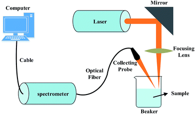
A schematic diagram of the experimental setup used for the LIF system is shown in Fig. 1; it mainly consists of a laser, a spectrometer and a computer system. The laser is a blue-violet semiconductor laser (Beijing Huayuan Tuoda Laser Technology Co., Ltd., Beijing, China) with the optical wavelength set at 405 nm and the maximum energy output of the laser is 150 mW. The laser is collimated by a focusing lens (focal distance 50 mm) and focused on the sample surface. The laser-induced plasma light signal is collected by using an optical fiber and is transmitted to the spectrometer (USB2000+; Ocean Optics Co., Largo, FL, USA) equipped with a 2048-pixel linear CCD array (Sony ILX511; Sony Corporation, Tokyo, Japan). The spectral range of the spectrometer is from 200 nm to 1100 nm.In this experiment, the relevant parameters were optimized as follows: the energy of the laser was 120 mW, the spectral range of spectrometer was 340–1021 nm, and the integration time was 1 ms. For the purpose of avoiding the influence of background light and other human factors on the experimental results, the experiment was carried out in a dark room. Fluorescence spectral data for all samples were collected and recorded using Spectra Suite software on a computer.30
2.2 Materials and samples
Considering that goaf water is the most harmful and most common source of water inrush, goaf water, sandstone water and their mixture were selected as the research object of this experiment. The experimental material was collected in the Huainan mining area of the Anhui Province on July 18, 2018. The goaf water and sandstone water were mixed in different volume ratios; 75 samples of each type were selected to form the following sample set:(1) Group A: single goaf water.
(2) Group B: the mixture of goaf water and sandstone water has a volume ratio of 4![[thin space (1/6-em)]](https://www.rsc.org/images/entities/char_2009.gif) :
:![[thin space (1/6-em)]](https://www.rsc.org/images/entities/char_2009.gif) 1.
1.
(3) Group C: the mixture of goaf water and sandstone water has a volume ratio of 3![[thin space (1/6-em)]](https://www.rsc.org/images/entities/char_2009.gif) :
:![[thin space (1/6-em)]](https://www.rsc.org/images/entities/char_2009.gif) 1.
1.
(4) Group D: the mixture of goaf water and sandstone water has a volume ratio of 2![[thin space (1/6-em)]](https://www.rsc.org/images/entities/char_2009.gif) :
:![[thin space (1/6-em)]](https://www.rsc.org/images/entities/char_2009.gif) 1.
1.
(5) Group E: the mixture of goaf water and sandstone water has a volume ratio of 1![[thin space (1/6-em)]](https://www.rsc.org/images/entities/char_2009.gif) :
:![[thin space (1/6-em)]](https://www.rsc.org/images/entities/char_2009.gif) 1.
1.
(6) Group F: the mixture of goaf water and sandstone water has a volume ratio of 1![[thin space (1/6-em)]](https://www.rsc.org/images/entities/char_2009.gif) :
:![[thin space (1/6-em)]](https://www.rsc.org/images/entities/char_2009.gif) 2.
2.
(7) Group G: the mixture of goaf water and sandstone water has a volume ratio of 1![[thin space (1/6-em)]](https://www.rsc.org/images/entities/char_2009.gif) :
:![[thin space (1/6-em)]](https://www.rsc.org/images/entities/char_2009.gif) 3.
3.
(8) Group H: the mixture of goaf water and sandstone water has a volume ratio of 1![[thin space (1/6-em)]](https://www.rsc.org/images/entities/char_2009.gif) :
:![[thin space (1/6-em)]](https://www.rsc.org/images/entities/char_2009.gif) 4.
4.
(9) Group I: single sandstone water.
All samples were kept from light and sealed to ensure that the experimental data were more realistic and reliable. Also, 60 samples per group were randomly selected and a total of 540 fluorescent spectral data were used as training sets. The remaining 25 samples for each group and a total of 135 fluorescent spectral data were used as the test sets.
2.3 1D CNN for LIF spectral data classification
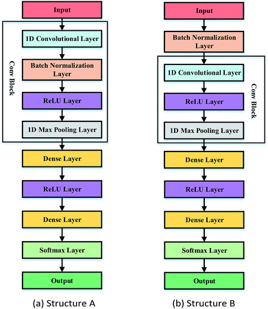
1D CNN, as an important branch of CNN, usually includes convolutional layers, activation layers, and pooling layers. According to the literature,27,31 we designed two typical structures of 1D CNN, as shown in Fig. 2. In structure A, each convolutional block (Conv Block) contains a batch normalization32 (BN) layer. However, the BN layer is not included in the Conv Block in structure B, and the BN layer is placed behind the input layer. In structure A as well as in structure B, it is easy to build a deep 1D CNN model by increasing the number of Conv Block. In addition, in order to choose the best structure, we have compared the performances of the 1D CNN model of these two structures in Section 3.1.Each component of 1D CNN is explained in detail as follows:
The input to 1D CNN for LIF spectroscopy classification is one dimensional and it contains the entire spectrum (input size is 1 × 2048).
In the Conv Block, the 1D convolutional layer is used to extract feature maps and different numbers of 1D convolutional filters of the same size are applied in each layer (stride of 1). As Conv Block goes deeper, the number of convolutional filters is doubled (starting from 16). The 1D convolutional layer can be expressed by
 | (1) |
BN is a technique for improving the performance and stability of neural networks, which can prevent gradient vanishing and over-fitting, as expressed by the following equation:
 | (2) |
Rectified linear units33 (ReLU) are used as a function of the activation layer that usually follows a convolutional layer or a fully connected layer. The ReLU can be described in eqn (3).
| f(x) = max(0, wx + b) | (3) |
Max pooling is the most commonly used pooling strategy, which is mainly used to reduce the number of dimensions in the feature maps and network parameters. Both structure A and structure B use max pooling with the size of 4.
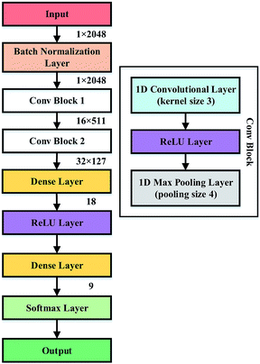
The upper layers of the CNN are fully connected by the dense layer, followed by the softmax layer. In the two structures of Fig. 1, two dense layers are used. The first dense layer has 18 outputs, and the second dense layer has the same number of outputs as the sample category (9). The softmax layer produces values in the range [0, 1] as classification confidence scores. Classification loss is calculated by comparing the confidence scores and true labels of samples. The softmax function and loss function are expressed as follows:
 | (4) |
 | (5) |
2.4 1D CNN training
Two typical structures of the 1D CNN model proposed above were initially developed on Keras (v 2.2.4), a lightweight library used to build and train deep-learning algorithms, with a TensorFlow (v 1.10.0) background. The models were built on a workstation with a GeForce RTX 2070 graphics processing unit (GPU) with 288 Tensor cores and 2304 GPU cores and 8 GB of GDDR6 memory in a Windows 10 environment.The training of the 1D CNN was performed using the Adam algorithm, which is a variant of stochastic gradient descent, for 1000 epochs with learning rate equal to 0.001, β1 = 0.9, β2 = 0.99, and ε = 1 × 10⁻⁸. For optimization, during training and testing, the batch size was set to 128.
3. Results and discussion
3.1 Original spectral data
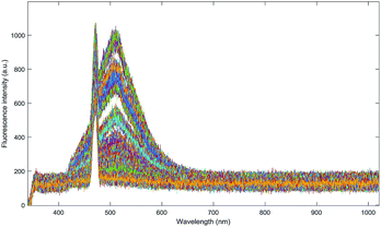
The spectral data of water samples were obtained by the LIF system; the spectral curves of all samples are shown in Fig. 3. It can be seen from the graph that the single goaf water and the single sandstone water are recognizable. However, it becomes indistinguishable when the two kinds of water are mixed together. There is a slight overlap of mixed water samples; thus, it is necessary to classify and identify with the help of chemometrics.3.2 Comparison of the two 1D CNN structures
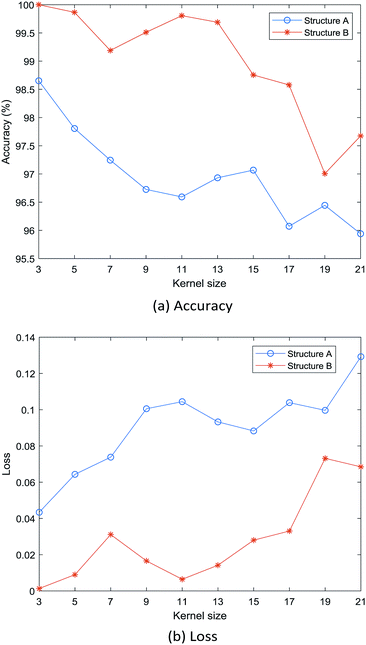
To test the two 1D CNN structures proposed in Section 2.3, the 1D CNN model with a Conv Block is constructed based on Fig. 2, and the classification performances of CNN models with two structures on the LIF spectra of mine water inrush are compared. By changing the size of the convolution kernel (from 3 to 21), accuracy and loss of 1D CNN models with two structures were recorded over 10 tests. The average accuracy and loss of 1D CNN models with two structures were calculated, as shown in Fig. 4. With the increase in the convolution kernel size, the accuracy of both structures shows a decreasing trend, and their loss tends to increase. This shows that the smaller the convolution kernel size, the easier it is to extract the appropriate features, which is helpful to improve the accuracy of classification. As can be seen from Fig. 4(a), the accuracy of the 1D CNN model of structure B is higher than that of structure A under the same convolution kernel size, which indicates that the 1D CNN model of structure B is more suitable for the LIF spectral classification of mine water inrush. Based on Fig. 4(a) and (b), we can determine that the 1D CNN of structure B should be used to construct an LIF spectral classification model for mine water inrush, and the kernel size of all convolutional layers in the model is set to 3.3.3 Optimization of the 1D CNN architecture
According to Fig. 2(b), 1D CNN models of different depths are constructed by concatenating different numbers of Conv Blocks. The model was trained and tested using LIF spectral data from mine water samples, and ten replicates were performed at each depth. The trainable parameters, training time, accuracy and loss were considered in the selection of the optimal 1D CNN model. The average results of the 10 trials are shown in Table 1. First, we compared the accuracy and found that the accuracy rate of the 1D CNN model with one or two Conv Blocks can reach a maximum of 100.00%. Then, comparing the loss of these two depth 1D CNN models, we found that the loss of the model that contains two Conv Blocks is smaller and the model is more stable. Next, we note that the number of trainable parameters of the 1D CNN model with two Conv Blocks is almost half that of the 1D CNN model with one Conv Block. In addition, as the model goes deeper, the training time gradually increases. Taking these indicators into account, the 1D CNN model with two Conv Blocks is more suitable for the classification of LIF spectroscopy data of mine water inrush.| Conv Blocks | Parameters | Time (epoch per ms) | Accuracy (%) | Loss |
|---|---|---|---|---|
| 1 Conv Block | 147 425 | 40.48 ± 0.27 | 100.00 ± 0.00 | 0.0013 ± 0.0007 |
| 2 Conv Blocks | 74 977 | 47.48 ± 0.40 | 100.00 ± 0.00 | 0.0006 ± 0.0002 |
| 3 Conv Blocks | 43![[thin space (1/6-em)]](https://www.rsc.org/images/entities/char_2009.gif) 745 745 |
51.66 ± 0.37 | 99.85 ± 0.16 | 0.0033 ± 0.0025 |
| 4 Conv Blocks | 48![[thin space (1/6-em)]](https://www.rsc.org/images/entities/char_2009.gif) 865 865 |
54.47 ± 0.34 | 99.94 ± 0.10 | 0.0041 ± 0.0031 |
3.4 Performance of the proposed 1D CNN model
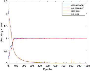
With the above results, we obtained the architecture of the 1D CNN model for LIF spectral classification for mine water inrush. As shown in Fig. 5, we can see more details about the 1D CNN model. The optimal architecture is a 2 Conv Block 1D CNN model: (1) Conv Block 1 comprises 16 filters with a kernel size of 3, and Conv Block 2 comprises 32 filters with a kernel size of 3. (2) Each convolutional layer is followed by an ReLU activation layer and a max pooling layer with the size of 3.Fig. 6 shows the changes in accuracy and loss under different epochs. The results show that as the number of epochs increases, the accuracy tends to increase, while the loss shows a decreasing trend. The accuracy and loss reached stable values after hundreds of epochs of learning when applied to the LIF spectroscopy of mine water inrush. The accuracy of both the training set and the test set was 100.00%, which indicated that the 1D CNN model can accurately identify 540 training set samples and 135 test set samples. In other words, the proposed 1D CNN model is feasible and effective for the classification of LIF spectroscopy data of mine water inrush.
3.5 Comparison with the traditional classification model
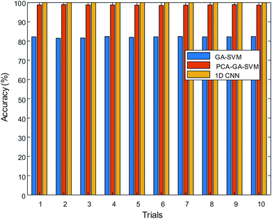
The performances of the GA-SVM model, PCA-GA-SVM model, and 1D CNN model are mainly compared here. Fig. 7 shows the accuracy of the three models under 10 trials. When the LIF spectroscopy data of mine water inrush are classified directly by using GA-SVM, the average recognition rate of all samples is 82.10%. On this basis, PCA is introduced to reduce the dimension of the original spectral data, and the average recognition rate increases to 98.77%. However, using the 1D CNN model for the classification of LIF spectroscopy data, the accuracy under all 10 trials is 100.00%. Compared with SVM models, the 1D CNN model has higher performance for LIF spectroscopy. At the same time, it can also be seen that SVM models have a certain dependence on the preprocessing of raw spectral data.3.6 Comparison with 2D CNN model
The input to the 2D CNN model is an image; thus, the fluorescence spectral image is drawn using the data of wavelength and fluorescence intensity. Based on Fig. 2, a similar structure 2D CNN model was constructed with the convolution kernel size set to 3 × 3 and the max pooling size set to 2 × 2. We increased the number of Conv Blocks to increase the depth of the network, while 10 repetitive tests were performed at different depths. Table 2 shows the average results of 10 repetitive trials. When using a 2D CNN model for recognition, it takes at least 3 Conv Blocks to achieve a 100.00% recognition rate. In other words, for the analysis of LIF spectroscopy of mine water inrush, the 2D CNN model needs a deeper network depth to achieve the recognition performance of the 1D CNN model. Comparing Tables 1 and 2, we can also find that the 2D CNN model has a longer training time and a larger number of trainable parameters at the same network depth. Therefore, the 1D CNN model is more suitable than the 2D CNN model for LIF spectral analysis of mine water inrush.| Conv Blocks | Parameters | Time (epoch per ms) | Accuracy (%) | Loss |
|---|---|---|---|---|
| 1 Conv Block | 558 525 | 93.75 ± 2.06 | 77.68 ± 7.33 | 0.3985 ± 0.1580 |
| 2 Conv Blocks | 253 917 | 114.88 ± 1.15 | 95.42 ± 9.30 | 0.0794 ± 0.1585 |
| 3 Conv Blocks | 125 085 | 124.11 ± 2.07 | 100.00 ± 0.00 | 0.0019 ± 0.0025 |
| 4 Conv Blocks | 125 469 | 137.77 ± 2.20 | 100.00 ± 0.00 | 0.0001 ± 0.0002 |
4. Conclusions
In this paper, we have proposed a 1D CNN model for the classification of mine water inrush from LIF spectroscopy, which not only exhibits outstanding performance, but also avoids the need for preprocessing raw spectral data. The 1D CNN model was designed with 1D convolution kernels, and various architectures were compared to identify the optimal architecture for the LIF spectral analysis of mine water inrush. The optimal architecture is a 1D CNN model with 2 Conv Blocks: Conv Block 1 contains 16 filters and Conv Block 2 contains 32 filters; the convolution kernel size of both Conv Blocks is 3. The 1D CNN model was trained and tested using the LIF spectroscopy of mine water inrush (goaf water, sandstone water, and their mixture), and all samples of training sets and test sets could be accurately identified. To validate the performance of the 1D CNN model, we compared it with the GA-SVM model and the 2D CNN model. Compared with SVM, we found that the 1D CNN model has higher accuracy, and using CNN to analyse LIF spectrum does not require preprocessing (such as PCA) of raw data. Compared to the 2D CNN model, the 1D CNN model has fewer Conv Blocks and less training time when achieving 100.00% recognition accuracy. In addition, the 1D CNN model can directly analyse the original spectral data, while 2D CNN needs to draw the spectral map based on spectral data before analysis. The present investigation considers the classification of mine water inrush from LIF spectroscopy using 1D CNN with 2 Conv Blocks. It will be interesting to extend the investigation to the identification by using a simpler architecture while considering designing a more versatile 1D CNN model that can be used for LIF spectroscopy of more substances.Conflicts of interest
There are no conflicts to declare.Acknowledgements
This work was supported by the National Safe Production Critical Incident to Key Technologies Science and Technology Project (No. anhui-0001-2016AQ), Anhui Province Natural Science Foundation for Youths (No. 1808085QE157) and National Safe Production Critical Incident to Key Technologies Science and Technology Project (No. anhui-0010-2018AQ). Suggestions of the anonymous reviewers which have improved the content of this presentation are also appreciated.Notes and references
- S. A. Shepeleva and V. V. Dyrdin, J. Min. Sci., 2011, 47, 660–663 CrossRef.
- S. Zhang, W. Guo and Y. Li, Arabian J. Geosci., 2017, 10, 503 CrossRef.
- F. Zhou, W. Ren, D. Wang, T. Song, X. Li and Y. Zhang, Int. J. Coal Geol., 2006, 67, 95–100 CrossRef CAS.
- Y.-P. Zheng, C.-G. Feng, G.-X. Jing, X.-M. Qian, X.-J. Li, Z.-Y. Liu and P. Huang, J. Loss Prev. Process Ind., 2009, 22, 528–532 CrossRef CAS.
- J. C. Pechmann, W. J. Arabasz, K. L. Pankow, R. Burlacu and M. K. McCarter, Seismol. Res. Lett., 2008, 79, 620–636 CrossRef.
- H. Gui, H. Qiu, W. Qiu, S. Tong and H. Zhang, Arabian J. Geosci., 2018, 11, 49 CrossRef.
- H. Ping-hua, W. Xin-yi and H. Su-min, Arabian J. Geosci., 2017, 10, 323 CrossRef.
- D. Jin, Z. Liu, Z. Liu and J. Chen, Coal Sci. Technol., 2013, 41, 25–29 Search PubMed.
- K. Peng, X. Li and Z. Wang, Environ. Earth Sci., 2015, 73, 7873–7888 CrossRef CAS.
- F. Hu, M. Zhou, P. Yan, J. Zhang, L. Wu and Y. Zhou, Spectrosc. Spectral Anal., 2018, 38, 2583–2587 CAS.
- G. Skrzypek, A. Mydłowski, S. Dogramaci, P. Hedley, J. J. Gibson and P. F. Grierson, J. Hydrol., 2015, 523, 781–789 CrossRef CAS.
- V. A. Galievsky, A. S. Stasheuski and S. N. Krylov, Anal. Chim. Acta, 2016, 935, 58–81 CrossRef CAS PubMed.
- S. Mounier, R. Redon, G. Nicolodelli and D. Milori, RSC Adv., 2017, 7, 56117–56122 RSC.
- D. I. Ellis, D. Broadhurst, S. J. Clarke and R. Goodacre, Analyst, 2005, 130, 1648–1654 RSC.
- P. Yan, M. Zhou, Q. Liu, K. Zhang and C. He, Spectrosc. Spectral Anal., 2016, 36, 243–247 CAS.
- Y. Wang, M. Zhou, P. Yan, F. Hu, W. Lai, Y. Yang and Y. Zhang, J. China Coal Soc., 2017, 42, 2427–2432 Search PubMed.
- J. Engel, J. Gerretzen, E. Szymanska, J. J. Jansen, G. Downey, L. Blanchet and L. M. C. Buydens, Trends Anal. Chem., 2013, 50, 96–106 CrossRef CAS.
- M. Zhou, W. Lai, Y. Wang, F. Hu, D. Li and R. Wang, Spectrosc. Spectral Anal., 2018, 38, 2262–2266 CAS.
- C. Liu, W. Hou and D. Liu, Neural. Process. Lett., 2017, 46, 1095–1119 CrossRef.
- D. George, X. Xie and G. K. Tam, Graphical Models, 2018, 96, 1–10 CrossRef.
- O. Abdeljaber, O. Avci, M. S. Kiranyaz, B. Boashash, H. Sodano and D. J. Inman, Neurocomputing, 2018, 275, 1308–1317 CrossRef.
- H. Cho and S. M. Yoon, Sensors, 2018, 18, 1–24 Search PubMed.
- Y. R. Tabar and U. Halici, J. Neural Eng., 2017, 14, 16003 CrossRef PubMed.
- S. Kiranyaz, T. Ince and M. Gabbouj, IEEE Trans. Biomed. Eng., 2016, 63, 664–675 Search PubMed.
- J. Acquarelli, T. van Laarhoven, J. Gerretzen, T. N. Tran, L. M. C. Buydens and E. Marchiori, Anal. Chim. Acta, 2017, 954, 22–31 CrossRef CAS PubMed.
- S. Malek, F. Melgani and Y. Bazi, J. Chemom., 2018, 32, 1–17 CrossRef.
- J. Liu, M. Osadchy, L. Ashton, M. Foster, C. J. Solomon and S. J. Gibson, Analyst, 2017, 142, 4067–4074 RSC.
- W. Yue, H. Hua, Y. Tian, J. Li, S. Jiang, C. Tang, S. Xu, Y. Ma, J. Ren and C. Bai, RSC Adv., 2017, 7, 43560–43566 RSC.
- M. J. Azarhoosh, F. Farivar and H. Ale Ebrahim, RSC Adv., 2014, 4, 13419–13429 RSC.
- B. Guan, A. Magenau, K. A. Kilian, S. Ciampi, K. Gaus, P. J. Reece and J. J. Gooding, Faraday Discuss., 2011, 149, 301–317 RSC.
- E. Urtnasan, J. U. Park, E. Y. Joo and K. J. Lee, J. Med. Syst., 2018, 42, 104 CrossRef PubMed.
- X. Han and Q. Dai, Applied Intelligence, 2018, 48, 142–155 CrossRef.
- V. Nair and G. E. Hinton, Proc. ICML, 2010 Search PubMed.
| This journal is © The Royal Society of Chemistry 2019 |

