Guided principal component analysis (GPCA): a simple method for improving detection of a known analyte

Abstract

There is increasing interest in the application of Raman spectroscopy in a medical setting, ranging from supporting real-time clinical decisions e.g. surgical margins to assisting pathologists with disease classification. However, there remain a number of barriers for adoption in the medical setting due to the increased complexity of probing highly heterogeneous, dynamic biological materials. This inherent challenge can also limit the deployment of higher level analytical approaches such as Artificial Intelligence (AI) including convolutional neural networks (CNN), as there is a lack of a ground truth required for training purposes i.e. in complex clinical samples. Principal component analysis (PCA) is an unsupervised data reduction approach (orthogonal linear transformation) that has been used extensively in spectroscopy for 30+ years, due to its capability to simplify analysis of complex spectroscopic data. However, due to PCA being unsupervised features will inherently appear mixed and their rank may vary between experiments. Here we propose Guided PCA (GPCA), a simple approach that allows PCA to be guided with spectral data to ensure a consistent rank of a key target moiety by the inclusion of a reference (guiding) spectrum to the data set. This simplifies analysis, increases robustness of PCA analysis and improves quantification and the limits of detection and decreases RMSE.

---

Introduction

The Deep Raman Spectroscopy (DRS) methods such as Spatially Offset Raman Spectroscopy (SORS) and Transmission Raman Spectroscopy (TRS), provide simple approaches to deeply probe the chemistry of scattering samples, which is inherently non-invasive and non-destructive.^1–4 Through a separation of illumination and collection zones on a sample, one can control the relative distributions of collected signal, from one that would ordinarily be surface dominated, to a distribution between surface and the signal at depth which is controlled by the separation distance used,⁵ or in the extreme with TRS, a whole volume between the collection and illumination zones can be probed. Due to the inherent biocompatibility of DRS i.e. non-ionising radiation, and complementarity of the information recovered, it can potentially complement existing approaches, such as mammography or ultrasound. When “contrast agents” such as gold surface enhanced Raman nanoparticles are used, they may also be potentially imaged using conventional whole body imaging such as CT/MRI.^6,7 DRS is rapidly being developed for a number of potential in vivo applications.⁸ However, for true clinical translation a number of barriers remain, including how the data is processed and analysed to optimally extract the disease specific signals and maximise sensitivity to disease, thus permitting disease diagnosis or monitoring.

Deep Raman approaches result in inherently more complex signals being retrieved than a linear combination of the component spectra, such as those found in reference databases^9,10 of pure spectra or from a 2D surface limited maps. A number of factors make absolute quantification remarkably challenging at depth with Raman spectroscopy. For example, analyte intensity of signal and crucially also its spectral profile can strongly vary due to several reasons, analyte location (depth or boundary proximity), distribution pattern, total sample size and shape as well as analyte concentration, sample heterogeneity, differential optical properties and fluorescence amongst others. Due to these complications the dominating variance observed relates to the optical properties of the matrix surrounding an analyte¹¹ and can often mean the signal of the analyte is complex to recover and quantify in a robust automated fashion.

Recent years has seen rapid expansion of algorithms available to analyse, quantify and classify spectral data (i.e. Raman and infrared spectra) under the expansive umbrella of AI and machine learning. These range from simple unsupervised approaches such as dimensionality reduction tools such as Principal Component analysis (PCA),^12,13 or clustering techniques i.e. K-means.^14–17 Supervised techniques routinely used include support vector machine (SVM), Random forest,¹⁸ K-nearest neighbour (K-NN).¹⁹ While more recently the cutting edge is represented by using Artificial neural networks (ANN),^9,19 such as deep convolutional neural networks, which have shown to produce a modest improvement of classification compared to other listed supervised approaches.⁹

Moreover, in deep Raman especially in real world applications, there is often a lack of spectra that could be used for training purposes e.g. analyte free control measurements. Often the spectrum is simultaneously dominated by the matrix chemistry and more significantly here the influence of its optical properties, which can limit the application of simple linear algorithms. A number of papers have demonstrated “relative” quantification is achievable at depth with Raman spectroscopy,^20–26 however, these works usually carefully control a number of parameters. As an example, in PCA, as the concentration of an analyte decreases it will appear gradually in lower rank eigenvectors as the variance it contributes to decreases. This means a single consistent principal component (PC) could not be used directly for analysis purposes, and it could be easy to over fit data, by including several PCs to resolve this effect. Here we demonstrate a novel approach, whereby in the unsupervised approach of PCA, a known pure spectrum of the analyte of interest is introduced to the analysis with the rest of the data guided PCA (GPCA). This enables a dramatic simplification of the analysis and sensitivity of analyte detection.

Materials & methods

All Transmission Raman measurements were carried out on an instrument similar to that described previously^20,27 and schematically represented in Fig. 1A. In summary, an 808 nm solid state laser (Innovative Photonic Solutions, Monmouth Junction, NJ, USA) was coupled to illumination optics via an optical fibre. A single 808 nm laser clean up filter (LL01-808-25, Semrock, Rochester, New York, USA) filtered the laser output prior to the beam being defocused to a ∼10–12 mm diameter beam on the sample surface. The sample stage platform consisted of a fused quartz window (2 mm thickness), which was held on a motorized stage (8MTF, Standa), providing full XY positioning control with a range of 102 mm in both directions. The Raman signal detected in transmission geometry was filtered by a single 808 nm edge (long pass) filter (BLP01-808R Semrock, Rochester, New York, US) placed prior to the collection lens (to reduce silica auto fluorescence from the optics). The collected light was coupled to a fibre bundle using a 50 mm diameter, 60 mm focal length lens. The bundle (Ceramoptec) had a circular array of fibres at the collection end and a linear array of fibres coupled into a Holospec 1.8i (Kaiser Optical Systems, Ann Arbor, Michigan, USA). The spectrometer contained a custom high dispersion grating (Kaiser Optical Systems) providing a spectral range of ∼600–1200 cm⁻¹ and a 1 mm slit with an effective spectral resolution of ∼15 cm⁻¹. The spectrometer was coupled to a deep depletion CCD detector (Andor BR-DD iDus 420) cooled to −70 °C to record the Raman spectra.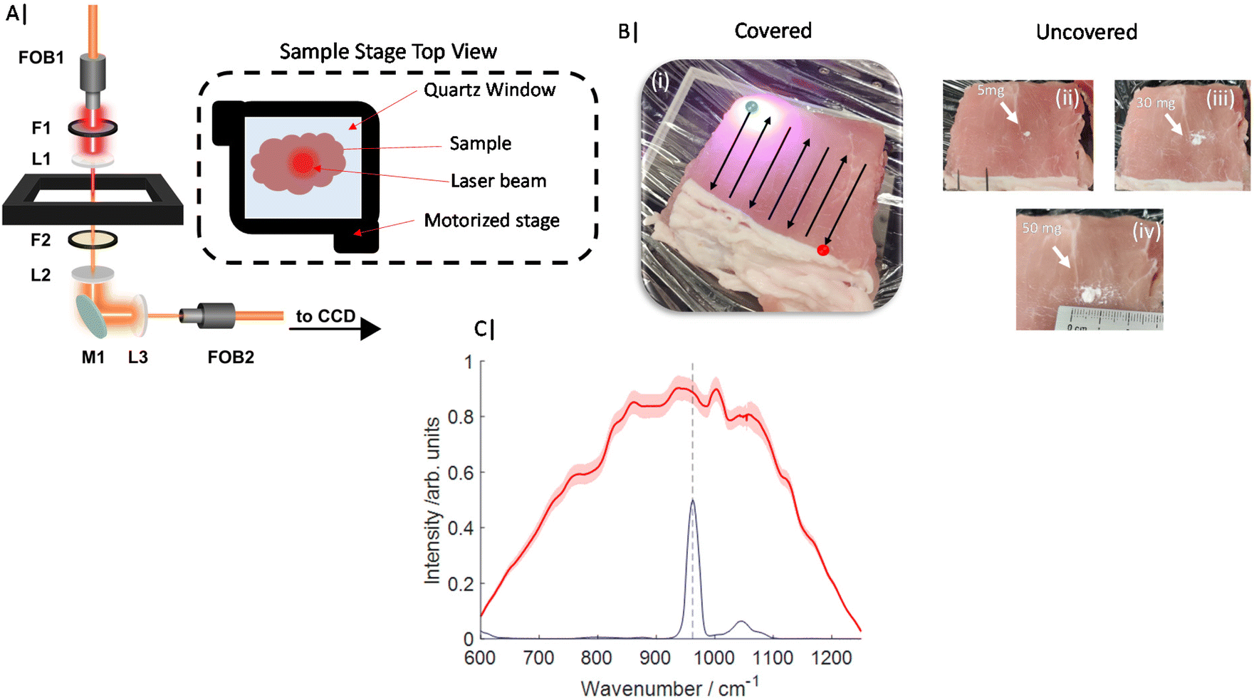

Fig. 1 (A) Schematic diagram of Transmission Raman optical beam path through ∼25–30 mm of tissue. (B) Images of porcine tissue (i–iv), covered sample and approximate raster pattern displayed (i) while uncovered samples and HAP deposits visible (ii–iv). (C) Average Raman spectra, red line with standard deviation (± shading), of 11 TRS maps containing 0 mg to 50 mg HAP, blue spectrum of HAP and dashed line indicates main Raman band (ν₁ PO₄) at 960 cm⁻¹.

Porcine tissue was obtained from a local supermarket (bacon slices) and cut into approximate squares ∼7 × 7 cm², and stacked to a range of total thicknesses of 22–30 mm. This tissue was first measured in the absence of any target analyte (inclusion). Calcium hydroxyapatite (HAP) (Sigma Aldrich) was then added directly in the approximate centre of the porcine tissue (in all dimensions, (x,y,z)) in increments of ∼5 mg over a range of 0–50 mg total (Fig. 1B) yielding 11 concentration points. Further, gelatin based breast tissue phantoms were also produced, which consisted of 5% gelatin (Sigma Aldrich) and 0.4% intralipid (Sigma Aldrich). Gelatin was added to distilled water and mixed under constant stirring and heating ∼50 °C for 10 minutes. Once dissolved the solution was cooled to approximately room temperature before intralipid was added and carefully mixed in. The solution was then left to set in a breast shaped mould with maximum dimensions (x,y,z) of 140 × 80 × 60 mm at 4 °C for ∼2 hours.

For Raman measurements of porcine samples, a laser power of 2 W was used, delivering a power density at the sample surface of ∼17 mW mm⁻². Porcine TRS mapping experiments were gathered from multiple spatial points across the sample, under the following conditions. Each experiment consisted of 11 Raman maps (Fig. 1C), where for each map the samples were rastered through the laser beam/collection path in a snake pattern with step size 2–3 mm. At each spatial location a TRS spectrum was acquired for 3 s (0.1 s × 30 accumulations). The entire experiment was carried out in triplicate i.e. 33 Raman maps in total.

Gelatin-intralipid breast phantoms were measured in a similar way; with a laser power of 4.5 W, delivering ∼39 mW mm⁻² and a step size of 3 mm was used, and total acquisition time was 3 s (0.5 s × 6).

Each Raman map was processed independently in Matlab 2017a following pre-processing outlined as follows. Firstly, a median filter was applied to the data to remove the presence of cosmic rays, the accumulated spectra collected at each spatial location were then averaged to leave one mean spectrum per spatial location. A linear baseline was then subtracted from the data prior to standard normal variate (SNV) normalisation, and rescaling to 0–1.

Initially standard PCA approaches were used to explore the variance in the datasets acquired to elucidate the impact of the matrix on the analyte signals. This was followed by the novel approach of GPCA, whereby the known target spectrum was additionally included in the input data matrix.

All principal component analysis (PCA) was undertaken in Matlab using built in functions utilising singular value decomposition with mean centring. For data where the GPCA process was used, the target spectrum of HAP was averaged, baseline corrected using a linear baseline and rescaled to [0–1], to match the data range of original input data. Data from each map was treated independently during analysis. It was only combined for illustrative purposes. All PCA data presented throughout is used from independent maps and not combinations of. For enhanced 2D visualisation of PC score maps (Fig. 2B & 3C), interpolation of data points with a spline function was carried out to 0.1 mm step.

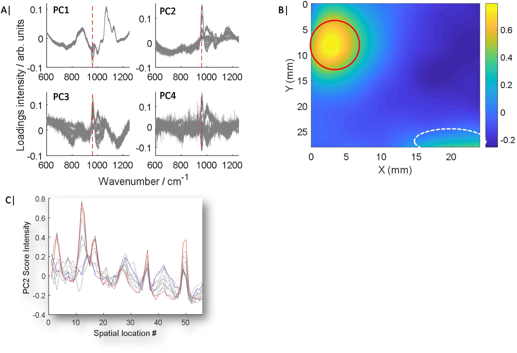Fig. 2 Conventional PCA. (A) PCA loadings plots of the first 4 components showing 11 results in each plot, covering each map collected from the samples containing 0 to 50 mg of HAP in increments of 5 mg. (B) Score plot of PC2 from the map with 50 mg HAP inclusion, HAP signal circled Red, distortion artefact circled white, intensity of the score value indicated by colour bar. (C) PC2 score values plotted for each of the 11 maps against each arbitrary spatial location (map data point), displayed as list in one dimension, with 0 mg HAP (blue), 50 mg HAP (red), all other HAP values (grey).

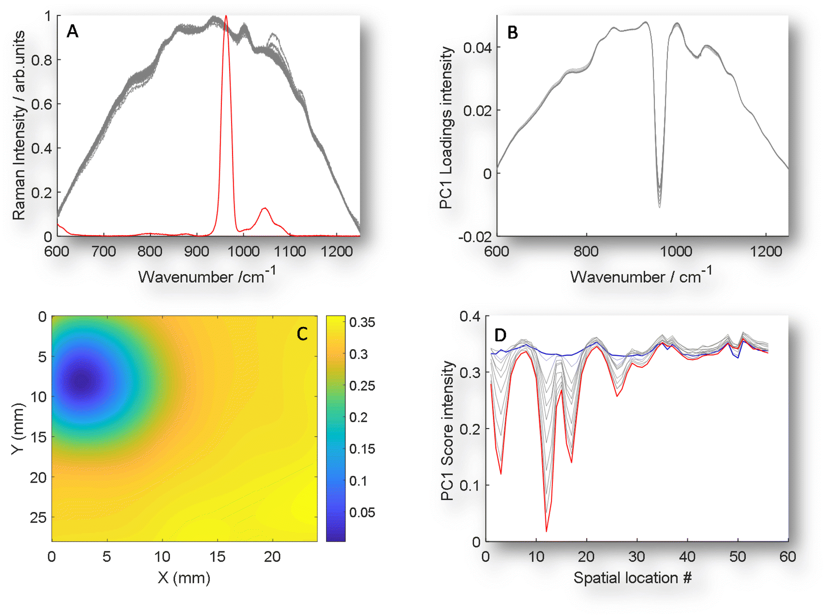Fig. 3 GPCA. (A) An example of TRS Raman data (grey) with the addition of the guided spectrum of an inclusion of pure HAP signal (red) on the same intensity scale. (B) Guided PC1 loadings plot of 11 TRS Raman maps with HAP ranging from 0 mg to 50 mg when data guided by the inclusion of scaled pure spectrum of HAP. (C) GPC1 scores organised in a 2D array to demonstrate special location of HAP for 50 mg inclusion, data interpolated to improve image for visualisation. Note that the PC1 loadings and scores are inverted when compared with PC2 plotted in unguided PCA data (Fig. 2). (D) GPCA scores plotted vs. location number for all 11 experiments, demonstrating increasing magnitude of scores for increasing HAP concentration.

Results and discussion

As is demonstrated in Fig. 1C, when only a small fraction of spectra contain a weak chemical feature of interest, this information can be lost in the averaging of the mixing of the inelastically scattered photons, making up the spectra from the full sample volume, thus making it challenging to detect and furthermore to accurately quantify an analyte. This can be even more challenging, when a ground truth is lacking i.e. zero control, a common likelihood in numerous real world applications.

Typically, PCA is used to simplify complex data sets where spectra are transformed into scores and loadings of decreasing importance. However, PCA is typically an unsupervised or unguided process, therefore as the analyte concentration or signal changes, so does its importance and ranking in Eigenvector space as is shown in Fig. 2A and S1.†Fig. 2A and S1† show overlaid loadings calculated independently using conventional PCA for 11 experiments, where the concentration of the analyte incrementally increases from 0 to 50 mg in ∼5 mg intervals. The presence of major features change in amplitude, sign (i.e. ±) as well as emergence point, i.e. low concentrations appear later in lower rank PCs while high concentrations appear sooner in higher rank PCs, with increasing inclusion concentration. Moreover, signals of interest, such as the ν₁ PO₄ mode of HAP at 960 cm⁻¹, are mixed with other interfering spectral features originating from the surrounding matrix that are of no interest; or worse are due to complexities such as differential self-absorption by the matrix distorting Raman spectral profiles.¹¹ The mixing of features can also lead to uncertainty of analyte location (Fig. 2B), even at the highest concentration of HAP (50 mg), while signal attributed to HAP is clearly visible (circled red) there are still distortion artefacts outside of this region circled white, which could be mistaken for HAP. The scores data of PC2 is also presented for 11 maps of increasing HAP concentration against arbitrary location (Fig. 2C), to better demonstrate expected changes with concentration and unconnected co-localised variance.

The concept of GPCA centres around introducing a known, pure analyte spectrum (guiding spectrum) numerically to the matrix data set, i.e. in this case transmission Raman mapping data (target matrix) (Fig. 3A) prior to PCA transformation. Following the introduction of the target spectrum (GPCA) the loading of PC1 is now clearly dominated by the target analyte (Fig. 3A), that provides a consistent relationship between HAP concentration and non-specific matrix variance. Moreover, a clearer scores 2D visualisation (Fig. 3C) is achieved and the scores visualisation no longer contains co-localised data that is not related to HAP, as was seen in the non-guided results (Fig. 2B).

The final advantage of this approach is seen in Fig. 3D, while previously the HAP concentration relationship was spread over multiple PCs (Fig. 2A and S1†), now a clear relationship is observed at relevant spatial locations in PC1 from 0 mg HAP to 50 mg (blue and red respectively). Further, to test whether any unrelated analyte could be introduced, we used a control demonstration, by including a guiding target spectrum of PTFE, that is not contained in the matrix or analyte that was used, see Fig. S2A & S2B.† While the loadings of the guided spectra dominate (S2A) as would be expected, the scores share no relationship with true chemical target, and becomes comparable to PC1 of unguided, conventional PCA.

A simple way to objectively evaluate the score data of each map with increasing concentration is through the dynamic range of the score value (Fig. 4A & C). This shows a correlation with increasing concentration and an R² ranging from 0.5–0.93 with conventional PCA, while GPCA shows a significantly more consistent performance 0.9–0.99. This is further reflected in its better prediction model performance (linear regression), while the limit of detection is 14.8 mg, this is reduced to 6.8 mg when GPCA is used, and an approximate halving of the RMSE from 4.2 to 2.02.

Fig. 4 (A) Conventional PC2 score range versus HAP concentration (mg) for three experiments (red circles, purple squares, pink diamonds). (B) Average HAP amount (mg) versus predicted HAP amount red circles (conventional PCR), pink line indicates limit of detection. (C) GPC1 score range versus HAP concentration (mg) for the same three experimental data sets used in (A) red circles, purple squares, pink diamonds. (D) Average HAP amount (mg) versus predicted HAP (guided PCA) amount red circles, pink line indicates overall limit of detection.

Finally, to demonstrate the versatility of the GPCA, a different type of phantom was used. This new phantom is of approximate breast size and shape that was constructed from gelatin and intralipid and contained three distinct deposits of HAP (Fig. 5A). The phantom is viewed from anterior to medial with respect to transmission geometry. While this is not a geometry whole breasts would be scanned in vivo (superior to inferior), it serves an illustration of the sampling capabilities of the technique. Previously, in porcine samples the z geometry i.e. thickness was approximately uniform and consistent between experiments, while this phantom has clear changes in thickness over any given mapped area. This has been demonstrated previously,¹¹ can introduce artefacts and complexity into the resulting signals due to differential self-attenuation of the Raman signal. Conventional PCA scores plots of the transmission Raman map (Fig. 5B & C) (PC1 and PC3) respectively, struggle to clearly separate HAP from other spectral features, as was observed in porcine samples i.e.Fig. 2B. However, GPCA (Fig. 5D) clearly enhances identification of the regions of interest that contain HAP. Demonstrating, that this approach is not confined to specific samples/signals and complexities.

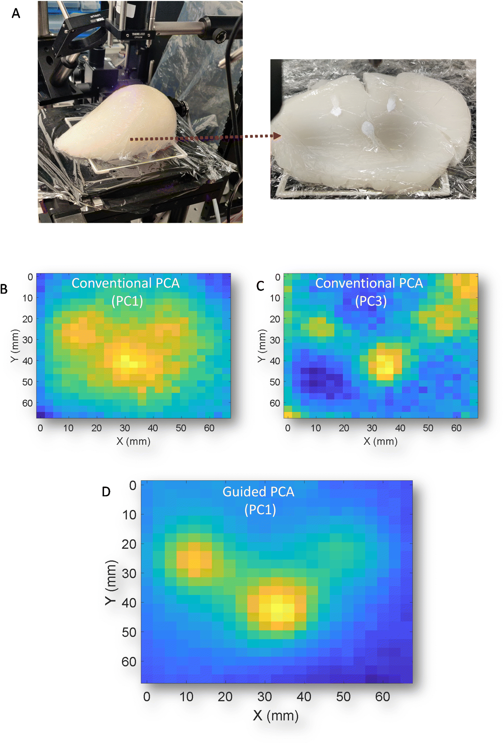Fig. 5 (A) (i) image of the whole gelatin/IL breast phantom, (ii) cross section of phantom showing three HAP inclusion positions. 2D scores plots from conventional PCA of PC1 (B), and PC3 (C) and PC1 using GPCA (D).

Conclusions

GPCA provides a simple, yet effective method, where provided a reference spectrum of the target analyte is known, its features can be promoted to a consistently higher-ranking principal component, described as a pure target analyte loading, enabling increased robustness with higher accuracy of quantification and improved LOD in complex matrixes. The method also avoids overfitting of data. This has the strong potential to impact on early disease diagnosis such as Raman detection of deep sited cancer lesions, thus improving the outcomes.

Conflicts of interest

The authors of this paper have no conflicts of interest to declare.

Acknowledgements

EPSRC grant EP/P012442/1 and EP/R020965/1 funded the work presented here. We would like to acknowledge Dr G. R. Lloyd, for valuable discussion on elements of the work presented here. Dr R Edginton for feedback and assistance of visual elements presented here. Finally, Dr L Clark for construction of the cast used to create gelatin phantom.

References

1. P. Matousek, Appl. Spectrosc., 2006, 60, 1341–1347.
2. P. Matousek, I. P. Clark, E. R. C. Draper, M. D. Morris, A. E. Goodship, N. Everall, M. Towrie, W. F. Finney and a W. Parker, Appl. Spectrosc., 2005, 59, 393–400.
3. S. Mosca, C. Conti, N. Stone and P. Matousek, Nat. Rev. Methods Primers, 2021, 1, 21.
4. F. Nicolson, M. F. Kircher, N. Stone and P. Matousek, Chem. Soc. Rev., 2021, 50, 556–568.
5. S. Mosca, P. Dey, M. Salimi, B. Gardner, F. Palombo, N. Stone and P. Matousek, Anal. Chem., 2021, 93, 6755–6762.
6. Kenry, F. Nicolson, L. Clark, S. R. Panikkanvalappil, B. Andreiuk and C. Andreou, Nanotheranostics, 2022, 6, 31–49.
7. P. Dey, I. Blakey and N. Stone, Chem. Sci., 2020, 11, 8671–8685.
8. P. Matousek and N. Stone, J. Biophotonics, 2013, 6, 7–19.
9. J. Liu, M. Osadchy, L. Ashton, M. Foster, C. J. Solomon and S. J. Gibson, Analyst, 2017, 142, 4067–4074.
10. J. De Gelder, K. De Gussem, P. Vandenabeele and L. Moens, J. Raman Spectrosc., 2007, 38, 1133–1147.
11. B. Gardner, P. Matousek and N. Stone, Analyst, 2021, 146, 1260–1267.
12. K. Pearson, London Edinburgh Philos. Mag. J. Sci., 1901, 2, 559–572.
13. I. Burstyn, Ann. Occup. Hyg., 2004, 48, 655–661.
14. E. Barshan, A. Ghodsi, Z. Azimifar and M. Zolghadri Jahromi, Pattern Recognit., 2011, 44, 1357–1371.
15. Y. Takane and M. A. Hunter, Appl. Algebra Eng. Commun. Comput., 2001, 12, 391–419.
16. Y. Xu and R. Goodacre, Metabolomics, 2012, 8, 37–51.
17. J. A. Westerhuis, T. Kourti and J. F. MacGregor, J. Chemom., 1998, 12, 301–321.
18. M. Sattlecker, R. Baker, N. Stone and C. Bessant, Chemom. Intell. Lab. Syst., 2011, 107, 363–370.
19. C. A. Meza Ramirez, M. Greenop, L. Ashton and I. ur Rehman, Appl. Spectrosc. Rev., 2021, 56, 733–763.
20. A. Ghita, P. Matousek and N. Stone, J. Biophotonics, 2018, 11, e201600260.
21. B. Gardner, P. Matousek and N. Stone, Analyst, 2019, 144, 3552–3555.
22. B. Gardner, P. Matousek and N. Stone, Anal. Chem., 2019, 91, 10984–10987.
23. B. Gardner, N. Stone and P. Matousek, J. Raman Spectrosc., 2020, 51, 1078–1082.
24. B. Gardner, N. Stone and P. Matousek, Faraday Discuss., 2016, 187, 329–339.
25. M. E. Berry, S. M. McCabe, S. Sloan-Dennison, S. Laing, N. C. Shand, D. Graham and K. Faulds, ACS Appl. Mater. Interfaces, 2022, 14, 31613–31624.
26. W. J. Olds, S. Sundarajoo, M. Selby, B. Cletus, P. M. Fredericks and E. L. Izake, Appl. Spectrosc., 2012, 66, 530–537.
27. A. Ghita, P. Matousek and N. Stone, Sci. Rep., 2018, 8, 8379.

---

Footnote

† Electronic supplementary information (ESI) available. See DOI: https://doi.org/10.1039/d3an00820g

---