Generative adversarial networks and diffusion models in material discovery

Abstract

The idea of materials discovery has excited and perplexed research scientists for centuries. Several different methods have been employed to find new types of materials, ranging from the arbitrary replacement of atoms in a crystal structure to advanced machine learning methods for predicting entirely new crystal structures. In this work, we pursue three primary objectives. (I) Introduce CrysTens, a crystal encoding that can be used in a wide variety of deep learning generative models. (II) Investigate and analyze the relative performance of Generative Adversarial Networks (GANs) and Diffusion Models to find an innovative and effective way of generating theoretical crystal structures that are synthesizable and stable. (III) Show that the models that have a better “understanding” of the structure of CrysTens produce more symmetrical and realistic crystals and exhibit a better apprehension of the dataset as a whole. We accomplish these objectives using over fifty thousand Crystallographic Information Files (CIFs) from Pearson's Crystal Database.

---

1 Introduction

Materials discovery is an enormous open problem in the field of materials informatics and a wide variety of techniques have been used to address it. Some methods include large-scale combinatorial synthesis simulations^1,2 to create crystals that are synthesizable and stable. However, in order for combinatorial synthesis methods to be successful, thousands or millions of compounds must be generated in order to identify useful candidates. Furthermore, known materials may only account for a minuscule fraction of the possible number of synthesizable and stable crystals.³ Discovering new structures in an efficient and effective way requires a method of processing enormous amounts of data, quickly identifying patterns that are present within the dataset, and extrapolating those patterns outside of the dataset so that new materials can be discovered. Generative models have been implemented for a variety of topics, including composition,^4–9 molecules,^10–23 and crystal structures.^24–40 In this work, we focus on crystal structure generative models.

Crystal generative models typically use variational auto-encoders (VAEs),^{27,31,35,37,41} generative adversarial networks (GANs),^{30,32,37,40,42} genetic algorithms,²⁸ or substitution.²⁹ One example of a crystal generative model based on VAEs is the Fourier-Transformed Crystal Properties (FTCP) representation.⁴¹ The FTCP representation is a crystal representation that not only incorporated both chemical and structural crystal properties but was invertible as well (property → chemistry + structure). When combined with a jointly trained VAE model, a probabilistic property-structured latent space was obtained that allowed for the generation of novel crystals with user-defined properties. Another important work in this area of study is the Crystal Diffusion Variational Autoencoder (CDVAE).³⁹ By leveraging a diffusion process that pushes atomic coordinates to lower energy states and iterates atom types to satisfy bonding preferences, CDVAE significantly outperforms past attempts to perform material generation. Furthermore, CDVAE was capable of optimizing crystals for a given property and reconstructing a material from its latent space representation. Many examples exist for GANs as well. Constrained crystals deep convolutional generative adversarial network (CCDC-GAN)³² uses a post-processing filtering criteria to remove compounds with large formation energies based on a cutoff threshold. In another example, crystal structure is represented in a lean fashion by a set of atomic coordinates and unit cell parameters, with significantly reduced memory requirements compared to a voxel-based generative model, iMatGen.³⁵ Physics Guided Crystal Generative Model (PGCGM)⁴⁰ expands on CubicGAN⁴² while using base site atoms with physics-guided loss functions. For example, structures with atoms that are too crowded or too far apart are penalized via two terms in the loss function. We also note that normalizing flows, another promising direction, have been used in some crystal structure contexts^38,43 including an application to molecular crystals.⁴³

In this work, we compare the use of Generative Adversarial Networks and Diffusion Models in unstructured crystal generation. We illustrate the shortcomings of GANs in this space and show that Diffusion Models may offer a very promising alternative to previous methods. Furthermore, we introduce a standardized and image-like crystal embedding representation (CrysTens) that can be used in a wide array of image generation models with relative ease and minimal changes.

2 Background

Creating an effective method of materials discovery is an extraordinarily important issue to address in the realm of materials science. Efficient materials discovery could revolutionize material science by not only yielding new materials but also by providing new insights into the different ways that crystal structures can form. Perhaps the most impactful outcome would be in the area of inverse design wherein materials are tailor designed to meet specific property criteria. Generating new stable crystal structures has proven a stubbornly difficult task, let alone to do so with targeted properties. An outstanding challenge in this area has been the periodic nature of crystal structures. Only recently were machine learning crystal representations developed that encode both the symmetry and composition information contained within the Crystallographic Information File (CIF).^44–47

New machine learning crystal representations that capture chemistry (composition) and structure (periodicity) are important because they then allow us to utilize machine learning algorithms to identify and exploit patterns in data. Even the most experienced materials scientist domain expert would be unable to fully comprehend and leverage all the patterns in high-dimensional materials data for hundreds of thousands of crystal structures, and then use the discovered patterns to generate novel materials. Instead, scientists have relied on very low-order approximations and simplifications for generating new materials. Or, alternatively, they have relied on screening down lists of already discovered materials to identify those candidates that most closely match the desired properties using empirical relationships or computational materials science techniques such as molecular dynamics, Density Functional Theory (DFT), etc. However, given the immense size of the chemical space that is believed to exist (10⁶⁰ materials) and our current microscopic subset of known materials (10⁵–10⁶ materials),³ it is unlikely that screening efforts alone are sufficient to find the new materials necessary to answer society's most pressing technological needs. Therefore it is abundantly clear that an intuitive and efficient method is needed to scan over the vast regions of untapped chemical space and select the groupings of materials it deems as stable and synthesizable.

Fortunately, machine learning and more specifically deep learning methods, have emerged as powerful complements to the human capacity for materials design.^48,49 Within the field of material discovery, generative machine learning models are currently being investigated by a wide variety of research teams.^39,44,50,51 Previously, the two most common types of generative machine learning models were the VAE and GANs. VAEs attempt to encode a sample of data into a lower dimensional latent space. The encoded samples are then decoded from latent space into potential new samples. However, VAEs differ from traditional autoencoders because they are simultaneously attempting to structure the latent space according to a predefined probability distribution. This makes VAEs an exciting candidate for efficient inverse design because materials that exhibit ideal properties may be located at the intersection of each property within latent space.^52,53

The other common generative machine learning model for material discovery is GANs. GANs differ from VAEs in several key ways. First, GANs are composed of two separate neural network architectures: the generator and the discriminator. The generator's task is to create realistic samples of whatever data distribution it is trying to model. In the case of this work, the generator is attempting to create realistic crystal structures. The discriminator's job is to differentiate between samples that are real (taken from the original dataset) or generated. The discriminator and generator train against each other, continually improving until training is finished and the generator can be separated and used to create realistic samples. By using an adversarial approach, the generator can construct its own probability distribution of the data instead of requiring a pre-defined probability distribution like those used within VAEs. Although the training of GANs is game-theoretic in nature, they are not guaranteed to converge to a Nash equilibrium⁵⁴ which can lead to performance issues. A more advanced variation of the traditional GAN is included in this work known as the Wasserstein GAN or WGAN. The differences between WGANs and GANs are discussed later.^55,56

Recently, however, with the success of OpenAI's DallE-2 ⁵⁷ and Google's Imagen,⁵⁸ Diffusion Models have quickly risen to achieve state-of-the-art performance for many types of generative modeling. Diffusion Models are inspired by non-equilibrium thermodynamics and operate by gradually destroying input training data by adding Gaussian noise (forward process) only to learn the transformations necessary to reconstruct each sample (backward process). By continually repeating this process, and incrementally adding more noise in each iteration, fully trained Diffusion Models are able to completely reconstruct a data sample from nothing more than noise. Diffusion Models take longer to train than GANs but do not suffer from many of the same deficiencies that GANs do such as mode collapse and extreme instability.

3 Methods

3.1 CrysTens representation

Past works such as iMatGen³⁵ and CCDCGAN³² focus on material generation within specific crystal systems. Our goal is to have the ability to generate a diverse range of different crystals and compositions. Since Pearson's Crystal Data (PCD) is not constrained to a single crystal system we chose it as the primary dataset of CIFs for this work. PCD contains over 140 000 unique CIFs, however, to fit the size constraints of CrysTens, the crystal embedding representation explained below (see Fig. 1 and 2), we filtered out any CIFs with more than 52 atoms in the basis. Additionally, we filtered out any erroneous or incomplete CIFs. Our final dataset contained 53 856 CIFs. Each CIF is used to create a CrysTens and these tensors are concatenated together to form our training set. For additional information about CIFs please see Appendix A.

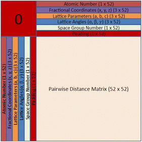Fig. 1 Layer 1 of the crystal representation containing symmetrical rows and columns for structural information and a pairwise distance matrix with relative distances between all atoms in the basis.

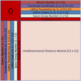Fig. 2 Layers 2–4 of the crystal representation containing the same symmetrical rows and columns for structural information, but also having a directional graph for each dimension: x, y, and z.

Finding a concise, efficient, and structurally informative representation for each CIF was an important step in the process of crystal structure generative modeling. Additionally, we wanted our representation to have image-like characteristics so that we could take advantage of high-performing image-generation models without a large amount of refactoring. After many iterations, including just simply listing the crystal structure parameters in a list, we eventually decided upon a representation that captured both the intricate parameters of each crystal as well as their interatomic components. The representation is a tensor of shape 64 × 64 × 4 and can be visualized in Fig. 1 and 2. The top twelve rows and leftmost twelve columns are symmetrical and list out all of the CIF-extracted information of a given crystal. The top (or leftmost) list is the atomic number of each of the atoms present in the crystal. They are listed from left to right (or top to bottom) until either fifty-two spots have been filled or the crystal has run out of atoms to place. If there is leftover space in the representation, zeros will be filled in for the remainder. Structures with more than 52 atoms in the basis are excluded. The same process is repeated for the three fractional coordinates (x, y, and z), the three lattice parameters (a, b, and c), the three lattice angles (α, β, and γ), and the space group number. Finally, a padding layer is inserted to separate the CIF-extracted information from the interatomic portion of the representation. For the first layer of the representation, the bottom-right 52 × 52 matrix is used to encode a pairwise distance matrix that relates each of the atoms together by their Euclidean distance. Within the latter three layers of the representation, a distance graph for each of the dimensions is represented to show the uni-dimensional relative distance between each atom.

The motivation behind the structure of this representation is to highlight the major components of crystal structures. There is a structural component that encodes symmetry, basis, and lattice information and an interatomic component that encodes the relative distances between atoms into the representation itself. With only the interatomic distances of a given crystal, it would be impossible to reconstruct the atomic numbers, space group, and various lattice parameters. Likewise, with only the structural components, it may be challenging for a convolution-based generative modeling algorithm to encode the relationships between various components which may lead to generated structures with unreasonable interatomic distances. Furthermore, there is a high degree of redundancy within our crystal structure representation by including both a pairwise distance matrix and unidimensional distance matrices as well as the repeating of lattice parameters, angles, and the space group number. The reason for this redundancy is that we would like to force the model to relate all of these different aspects in a way that can give rise to a greater ability to recognize and utilize crystal patterns within the PCD dataset during generation and a higher degree of noise mitigation during post-processing when all of these generated values are averaged. The primary strength of the CrysTens representation is that the structural aspects of a given crystal are fully encoded by including both the pairwise distance matrix and the distance graphs. This is desirable when using convolution-based image-generation models as they perform best when there is structurally informative data in the representation. Also, this gives the models that are trained on our representation several ways in which they can learn the patterns present in a crystal dataset. The repetition of lattice parameters, lattice angles, and the space group number present in our crystal representation may be viewed as a potential drawback as the model is forced to learn the same information several times, however, we chose to move forward with this representation as we felt it was the most natural representation.

We selected 64 as the length and width of each of our layers because of the commonly used deep learning heuristic of selecting powers of two. It could easily have been another value, however, the focus of this work is to show the structure of the CrysTens representation rather than the numerical intricacies or optimization of the representation. Furthermore, since 64 was selected and there are eleven different parameters plus a padding layer, only crystal structures with 52 atoms or less were selected for training and analysis. We redundantly included both the pairwise distance matrix and the three dimensional graphs to fully capture all of the different structural aspects of a given crystal structure, however, the representation can be changed to fit given constraints. We anticipate that future work could add layers to encode aspects related to chemistry such as the Oliynyk, magpie, mat2vec vector constituents in order to ensure realistic atom assignment.

3.2 Crystal reconstruction

Once we have trained a model with the CrysTens representation, it would be desirable to transform the output of each model at inference time back into a CIF for visualization and analysis purposes. The process of transforming back from the CrysTens representation can also provide insights into the level of “understanding” of the representation itself that each model displays. CrysTens representations generated from CIF files are by definition symmetric, but CrysTens' that are output from generative models are not necessarily symmetric due to the stochastic nature of deep learning algorithms. Instead, we found that even our most symmetrical generated CrysTens' had a small amount of noise that was mitigated by the redundancy of our representation.

Given a generated CrysTens, there will be a number of atoms that it will have predicted to be present in a crystal. We will refer to this value as A, and 0 < A ≤ 52 due to the nature of the current CrysTens representation. If the generative model was able to understand the symmetrical relationship within the CrysTens representation, then it will have A non-empty columns from left to right, and A non-empty rows from top to bottom for each of the four layers. Similarly, the single-valued structure parameters such as the lattice parameters (a, b, c), the lattice angles (α, β, γ), and the space group number will be repeated 2A times for each layer, a total of 8A occurrences. These values can be averaged to find the value that will ultimately be used when generating the output CIF. The variance among these repeated values is a good indicator of whether a given model “understands” the structure of the representation. If almost all 8A space group numbers are between 219 and 221, then there is a good chance that the model intended on a space group number of 220 and knew where to place these values. Generated CrysTens representations with small variances between values that are meant to be the same tended to produce more symmetrical and better-looking crystals, shown in Results. However, if there is a space group number spread between 110 and 220 there is a very good chance that the model is not able to pick up on the relationship between the different space group rows and columns, and the quality of the finalized crystal is likely to reflect that. Values that do not represent a single value throughout the entire CrysTens such as atomic number or fractional coordinates are instead only repeated a total of 8 times (two times for each layer) because each one corresponds to a single atom. The same variance check can be performed on each of these values as well.

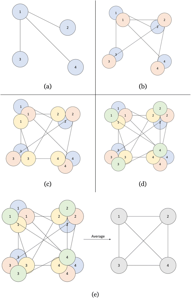
However, the single best indicator of model performance comes from the use of the directional graphs (layers 2–4). Each spot in the directional graphs represents the relative difference between two atoms in all three dimensions. Therefore, with the knowledge of one atom and its relationship to another atom with the direction graph, the second atom's location can be deduced. Therefore, if we have 10 atoms predicted in a CrysTens representation, each with their respective fractional coordinates and a directional graph relating each of them, we can have 10 “guesses” as to where a given atom is supposed to be in the crystal (one guess from its own x, y, z coordinates and nine guesses from the relative distances of other atoms). This process is highlighted in two dimensions in Fig. 3. If there is a high degree of consistency between all of the coordinate predictions, the crystal that is produced tends to be more symmetrical and realistic. The average of the coordinate predictions for each atom is ultimately chosen as the point where a given atom is placed during the CIF reconstruction. Furthermore, with these reconstructed coordinates, a pairwise distance matrix can be created and compared to the generated pairwise distance matrix in layer 1 as an additional metric for model performance.

Fig. 3 (a) The location of atom 1 is chosen based on its predicted fractional coordinates (x₁, y₁, and z₁). The location of atom 2 is chosen by taking atom 1's location and adding the relative distance between atom 1 and atom 2, found in layers 2–4 of the CrysTens representation (x₁ + Δ_2,x, y₁ + Δ_2,y and z₁ + Δ_2,z) The locations of atoms 3 and 4 are found the same way. (b) The location of atom 2 is chosen based on its predicted fractional coordinates (x₂, y₂, and z₂) and predictions for atoms 1, 3, and 4 are found using layers 2–4 of the CrysTens representation. (c) The same method is applied. (d) The same method is applied. (e) Finally, each of the positions are averaged and the final fractional coordinates are used in the construction of each CIF.

We are now left with an averaged value for the lattice parameters, lattice angles, and the space group number. We also have an average value for each of the coordinates of a given atom. In order to produce clean crystals that do not reflect the noise of the generative model, we added a few more post-processing steps.

As far as the atomic numbers are concerned, we found that even when there was low variance within the predicted atomic numbers we could still observe lists of atomic numbers such as (12.2, 12.6, 12.4, 12.5, 7.7, 7.4, 8.4, 8.5). When rounded to the nearest atomic number, this list would reflect (12, 13, 12, 13, 8, 7, 8, 9) → (Mg, Al, Mg, Al, O, N, O, F) instead of the list that would correspond to rule of parsimony: (12, 12, 12, 12, 8, 8, 8, 8) → (Mg, Mg, Mg, Mg, O, O, O, O). In order to rectify this inconsistency, we elected to use K-means clustering for the atomic numbers. For similar reasons, we chose to use K-means clustering for the coordinate values of x, y, and z across the different atoms. Now we could create a list of elements in the CIF as well as another list corresponding to their atomic positions. Using the averaged values from above, a Pymatgen lattice object can be constructed which is then used in conjunction with the element and coordinate lists to create a Pymatgen structure object. The structure object can be used to create a CIF.

3.2.1 Post-processing summary. ^• Generate CrysTens from a model with A non-empty rows/columns.

^• For lattice parameters, lattice angles, and space group number, average all 8A instances of each and use averages in the generated CIF.

^• For each atomic number assignment, it will be repeated 8 times (2 times per layer). Average these 8 instances for all A atomic number assignments.

^• Perform K-means clustering on averaged atomic number assignments, setting each to its centroid value and rounding to the nearest whole number for the final list of atomic number assignments.

^• For atomic position assignments in each dimension, it will be repeated 8 times (2 times per layer). Average these 8 instances for all A unidimensional atomic position assignments.

^• Perform the process described in Fig. 3.

^• Perform K-means clustering on averaged atomic position assignments, setting each to its centroid value and rounding to the nearest whole number for the final list of atomic position assignments.

^• Construct CIF with lattice parameters, lattice angles, space group number, atomic number list, and atomic position list.

3.3 Model overviews

3.3.1 Vanilla generative adversarial networks. Generative Adversarial Networks depend on an adversarial approach to generate new data. The two neural networks that GANs are composed of, the generator and the discriminator, work against each other. The generator attempts to generate realistic data and the discriminator attempts to differentiate between generated and real data. In order for the discriminator to predict whether a given sample is real or fake, a sigmoid activation function is used. When a prediction is above or equal to 0.5 on the sigmoid function, the sample is labeled as real, and if the prediction is below 0.5, the sample is labeled as fake or generated. The more sure the discriminator is of its prediction, the more it will tend to predict closer to 1 or 0 as opposed to around 0.5.

The major shortcoming associated with the sigmoid activation function directly corresponds to the difficulty of the tasks assigned to the two neural networks. It is far easier to classify if a given sample is real or fake than it is to generate an entirely new sample. During the initial training epochs, before the generator has had any time to calculate the weights necessary for accurate sample generation, it will produce samples that are very obviously fake. When the discriminator has to decide between something that is clearly real and something that is obviously fake, it will start performing very well and will begin predicting with higher confidence (a value closer to either 1 or 0).

When plotted on a sigmoid activation function, low confidence predictions correspond to a large gradient (closer to 0.5) while high confidence predictions correspond to a progressively diminishing gradient (closer to 1 or 0). A prediction plotted within the large gradient zone of a sigmoid activation function corresponds with more-useful information being given back to the generator about how to improve its weights. Inversely, a prediction plotted within the diminishing gradient zone will provide the generator with less-useful information. The more confident the discriminator becomes with its predictions, the more the gradient and the usability of the information coming from the discriminator will be decreased (vanishing gradient problem). This leads to a repeating cycle where the discriminator continually improves and the performance of the generator ultimately stagnates.

3.3.2 Wasserstein generative adversarial networks. To rectify the issue mentioned in the previous section, researchers have implemented a technique that takes advantage of the Earth Mover's Distance (EMD). EMD is a method of understanding the dissimilarity between two multidimensional sets of data samples. In our case, the two data sets are the real CrysTens' constructed from PCD and the samples produced by the generator. The theoretical “distance” between the two sets of data samples can be used to construct a loss function called the Wasserstein Loss, and the GANs that take advantage of this are known as Wasserstein GANs (WGANs). Using Wasserstein Loss, WGANs no longer need to predict if a sample is real or fake based on a probability between 0 and 1. Rather, the mathematics of the EMD equation allows WGANs to instead predict the “realness” of a sample. The discriminator is replaced with a critic function by changing the last layer from a sigmoid activation function to a linear activation function. This adjustment to the training scheme of the GAN rectifies the problem discussed earlier because the linear activation function has the same slope no matter what x-value is used.

Since the slope of the line is constant with respect to the relative performance between the critic and the generator (there is no low-gradient zone), the critic will never cease to grant the generator with useful data in terms of how to adjust its weights in order to produce more realistic samples.

3.3.3 Diffusion models. Unlike GANs, Diffusion Models do not depend on adversarial processes to generate outputs. Diffusion Models generate data based on non-equilibrium thermodynamics. Diffusion Models are composed of two separate stages: the forward and reverse diffusion processes. The forward diffusion process is responsible for the addition of Gaussian noise to a given sample while the backward diffusion process is the reconstruction of a sample from a noisier sample. Diffusion Models operate on a series of time steps, from 1 to t, where an increased time step indicates another addition of Gaussian noise. This process is treated as a Markov chain, where the sample at time step t only depends on the sample from time step t − 1. The forward process is fixed, however, the model attempts to learn the necessary operations to perform on a given sample at time step t to reconstruct the sample at t − 1. Once training is complete, the model should be able to generate a sample similar to those within the original distribution from complete Gaussian noise. While GANs may suffer from mode collapse and instability during training, Diffusion Models allow for stable training of large models on diverse data.⁵⁹ While sampling from Diffusion Models requires many more forward passes when compared to GANs single-pass during inference, this allows for refinement of outputs and is not a major drawback for this particular use.^60,61

4 Results

Several models from each category (Vanilla GANs, WGANs, and Diffusion Models) were trained using the CrysTens representations in an attempt to understand which deep learning method should be explored further for material discovery. The models were evaluated on several different metrics and we found a strong correlation between a general “understanding” of our representation and the output CIFs that were received. The GAN and WGAN used were custom convolution-based models. The Diffusion Model is the model found at https://github.com/lucidrains/imagen-pytorch. The details and hyperparameters of each model can be found in Appendix B.

Table 1 is used to show the ability of each model to capture the symmetrical characteristics of the CrysTens' structure. The average variance among each repeated parameter, angle, space group number, and fractional coordinates in the CrysTens representation for one thousand generated CIFs was calculated. Table 2 shows the average agreement between absolute and relative coordinates in a given CrysTens as to where to place each atom, as well as the average difference between the reconstructed pairwise distance matrix and the generated pairwise distance matrix for one thousand generated CIFs.

Table 1 Comparison between GANs, WGANs, and Diffusion Models on CrysTens lattice parameters, lattice angles, space group, and fractional coordinate variance^a

Model	σ Parameter ^2	σ Angle ^2	σ Spacegroup ^2	σ Fractionalcoordinates ^2
a One-thousand CrysTens representations were generated and the variance was averaged over all of them.
GAN	582.23	1338.11	6322.1	5.57 × 10^−2
WGAN	31.18	695.03	3024.27	5.9 × 10^−2
Diffusion	3.5 × 10^−1	8.46 × 10^−1	4.56	4.36 × 10^−4

---

Table 2 Comparison between GANs, WGANs, and Diffusion Models on CrysTens coordinate agreement and pairwise distance matrix difference^c

Model	ΔCoordinate/atom^a	Σ(ΔPairwise)/atom^b
a The difference between the “absolute” x, y, and z values predicted and the “relative” position predicted by the direction graph. b The sum of the difference between the reconstructed pairwise distance matrix (by the final coordinates) and the generated pairwise distance matrix in layer 1 of CrysTens. c One-thousand CrysTens representations were generated and the values was averaged over all of them.
GAN	9.62 × 10^−2	3.84
WGAN	1.37 × 10^−2	2.49
Diffusion	5.51 × 10^−4	4.73 × 10^−1

---

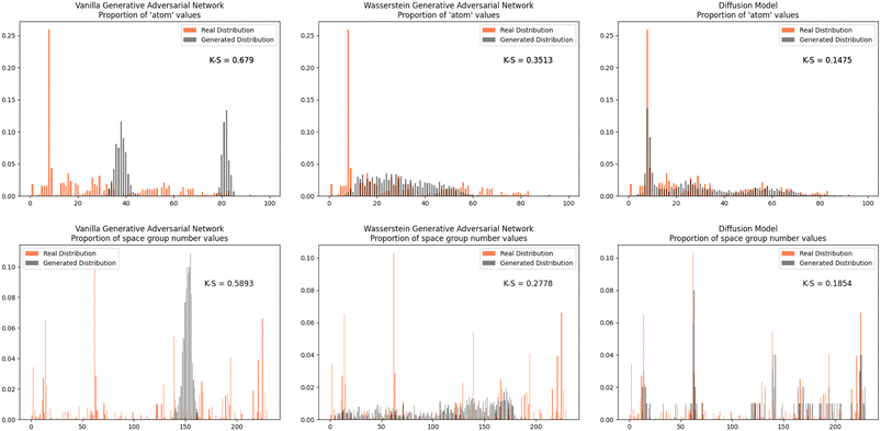
Furthermore, we wanted to investigate how well each model modeled the PCD dataset as a whole. To do this, the distribution proportions of the parameters, angles, space group number, and atomic numbers were found for the 53 856 CIFs in our dataset. The same distribution proportions were calculated for the set of one thousand generated CIFs generated by each model and the Kolmogorov–Smirnov (K–S) statistic was calculated for comparison between the distributions of real and generated parameters. Similar distributions will have a low K–S statistic (Fig. 4–6).

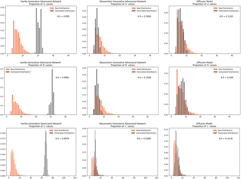Fig. 4 The distribution proportion for the parameters a, b, and c for the real CIFs vs. the generated CIFs.

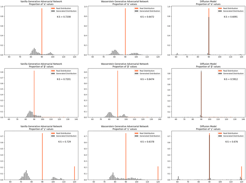Fig. 5 The distribution proportion for the angles α, β, and γ for the real CIFs vs. the generated CIFs.

Fig. 6 The distribution proportion for the space group numbers and atomic numbers.

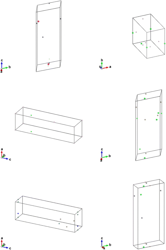
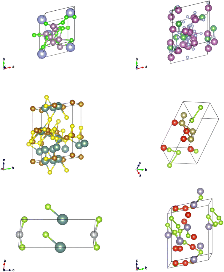
To investigate whether the correlation between CrysTens symmetry and CIF quality was reflected on an external metric, we used the Crystal Graph Convolutional Neural Network (CGCNN) to calculate the distribution of predicted formation energy, final energy, band gap, bulk moduli, shear moduli, Fermi energy, and Poisson ratio for the real CIFs as well as the generated CIFs for each model (Fig. 7).⁶² The K–S statistic is calculated for comparison between the distributions of real and generated predicted properties. This metric explores a model's quantitative ability to create CIFs that adhere to the real CIF property distributions without ever being exposed to CGCNN predictions during training. We recognize that CGCNN serves as an imperfect surrogate model because it was trained on a different dataset. Because of this, the CIF distributions will not match reality exactly, however, this metric provides proxy model performance indicators nonetheless. We also evaluated the CIFs based on their predicted energy above convex hull. In order to do this, we used M3GNet to predict the formation energy of a given crystal and compared it to the convex hull of its crystal system, which was created by PyMatGen (Fig. 8). M3GNet is a materials graph neural network that incorporates three-body interactions.⁶³ The energy above convex hull calculation code is found in https://github.com/michaeldalverson/CrysTens. Finally, several generated CIFs from each model are shown to showcase the visual differences in the generated crystal quality (Fig. 9–11). The produced CrysTens' used for evaluation, used 3-means clustering for the atomic numbers and 6-means clustering for the potential distinct x, y, and z coordinates (see Post-processing summary). Manually selecting the K value before generating one thousand CIFs from each model does damage the overall performance of each model. This constraint was applied to each model however, and thus a comparison between each model with this limitation is valid.

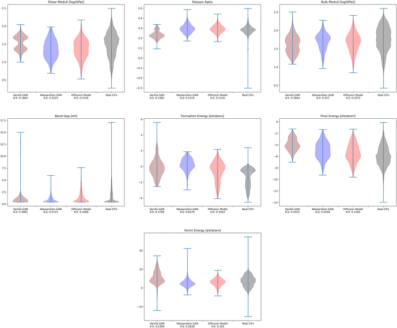Fig. 7 The distribution of CGCNN predicted values for the real CIFs and the CIFs generated by each of the models.

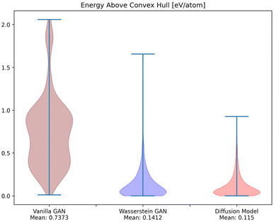Fig. 8 The distribution of M3GNet-predicted energy above convex hull for the CIFs generated by each of the models.

Fig. 9 CIFs generated from the Vanilla Generative Adversarial Network Model.

Fig. 10 CIFs generated from the Wasserstein Generative Adversarial Network Model.

Fig. 11 CIFs generated from the Diffusion Model.

5 Discussion

The Diffusion Model outperformed Vanilla GAN and WGAN by several orders of magnitude in minimizing variance across lattice parameters, lattice angles, space group number, and fractional coordinates as well as the agreement between absolute and relative fractional coordinates and the pairwise distance matrix difference metric. The Vanilla GAN was orders of magnitude worse than both the WGAN and Diffusion Models. We hypothesized that low variances across parameters, angles, space group number, and fractional coordinates and low differences between relative and absolute fractional coordinates would correspond to better performance in other metrics as well. With this hypothesis, we were expecting to see the Diffusion Models create CIFs that shared a higher degree of similarity with the real PCD distribution than the WGAN and GAN as well as produce higher quality CIFs.

When the distribution of lattice parameters, lattice angles, space group numbers, and atomic numbers of each model was checked against the values in the real distribution, we found that once again, our Diffusion Model performed best. In all areas, Diffusion Models performed exceedingly well, even capturing the peaks in the distribution of space group and atomic numbers (see Fig. 6), WGANs were not able to do this and Vanilla GAN distributions were even worse with indications of severe mode collapse.

Using pre-trained CGCNN models, several material properties were predicted for each CIF. The distribution of each predicted property for each model was compared against the distribution of that property across real CIFs. The violin plots qualitatively show the comparison between the generated and real CIF distributions. By looking at the shape of the violin plots with respect to that of the real distribution and the K–S statistics, it can be seen that both Diffusion Models and WGANs were capable of approximating the real distribution of each predicted property to an adequate degree, while GANs struggled, once again showing the mode collapse that occurred. In every case, Diffusion Models produced a CIF distribution that had a lower K–S statistic than both GANs and WGANs, implying a more similar distribution to the real CIFs in PCD. When investigating the M3GNet predicted energy above convex hull, we found that Diffusion Models and WGANs both performed far better than GANs. Diffusion Models, on average, produced CIFs that had a lower energy above convex hull than WGANs.

Finally, a set of CIFs was shown for each model. The CIFs generated by the Vanilla GAN represented exactly what was exhibited in the parameter and CGCNN prediction distributions. All of the CIFs found had very similar parameters and space group numbers. There was an extremely low degree of symmetry and general realness. Furthermore, the bounding boxes outlined by the lattice parameters were enormous in every CIF that we observed. The lack of “understanding” of CrysTens that the Vanilla GAN showed reflected in the CIFs it was capable of producing.

The CIFs produced by our WGAN were a positive shift in the correct direction. There was far more variability in the lattice parameters, lattice angles, space groups, and elements present when CIFs were generated. There are echoes of symmetrical components visible within the CIFs, however, symmetry would not be a word used to describe these CIFs. There is clearly room for improvement for the CIFs generated from our WGAN.

The CIFs generated by our Diffusion Models not only have a diverse set of lattice parameters, lattice angles, space group numbers, and elements present, but they are symmetrical and realistic looking. Although the CIFs produced are not perfect, there is a clear distinction between the CIFs produced by our Diffusion Model and our WGAN.

6 Further validation

Given the success of our Diffusion Model on our metrics, we attempted to validate some of the CIFs generated by our Diffusion Model. M3GNet can be used as an additional predictor of formation energy for all of the CIFs generated by the Diffusion Model (Fig. 12).⁶³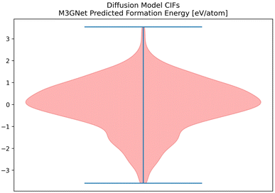

Fig. 12 The distribution of formation energy, as predicted by M3GNet for the CIFs generated by the Diffusion Model.

Among the top 35 CIFs with the lowest M3GNet-predicted formation energy, we selected 6 of them to be rigorously analyzed using Vienna Ab Initio Simulation Package (VASP). To prepare the 6 CIFs, slight manual tuning was applied after post-processing to maximize the likelihood that the structure would be realistic and stable. The manual tuning consisted of rounding fractional coordinates to more probable locations such as (0.011, 0.502, 0.009) → (0.0, 0.5, 0.0), and correcting potentially erroneous atomic number assignments as a result of the rounding within post-processing (36:Kr → 37:Rb). In order to evaluate the stability of the 6 selected CIFs, we performed a series of 4 successive relaxation calculations for each crystal structure. Running multiple relaxation calculations using a conjugate gradient algorithm helps ensure the ions have converged to their instantaneous ground state in the primitive unit cell. We used the Perdew–Burke–Ernzerhof exchange–correlation functional modified for solids, a break condition of 10⁻⁵ eV for the ionic relaxation loop, and a smearing width of 0.1 eV. Atomic pseudopotentials developed by G. Kresse and Peter Blöchl were used.^64,65 All the calculations were performed with a cutoff energy of 400 eV for the plane-wave basis set, the k-point grid as 3 × 3 × 3,⁶⁶ and each relaxation calculation typically included about 20 self-consistent field (SCF) iterations to reach the energy cut-off value. We calculate the free energy for the pre-relaxed CIFs and for the relaxed structures, and we calculate the external pressure after each of the relaxation calculations to evaluate their stability. The calculated free energy for the pre-relaxed structures (E₀), after the 4th relaxation (E₄) and the external pressure on the unit cell in kb after the 1st (P₁) and 4th (P₄) relaxation are shown below (Fig. 13).

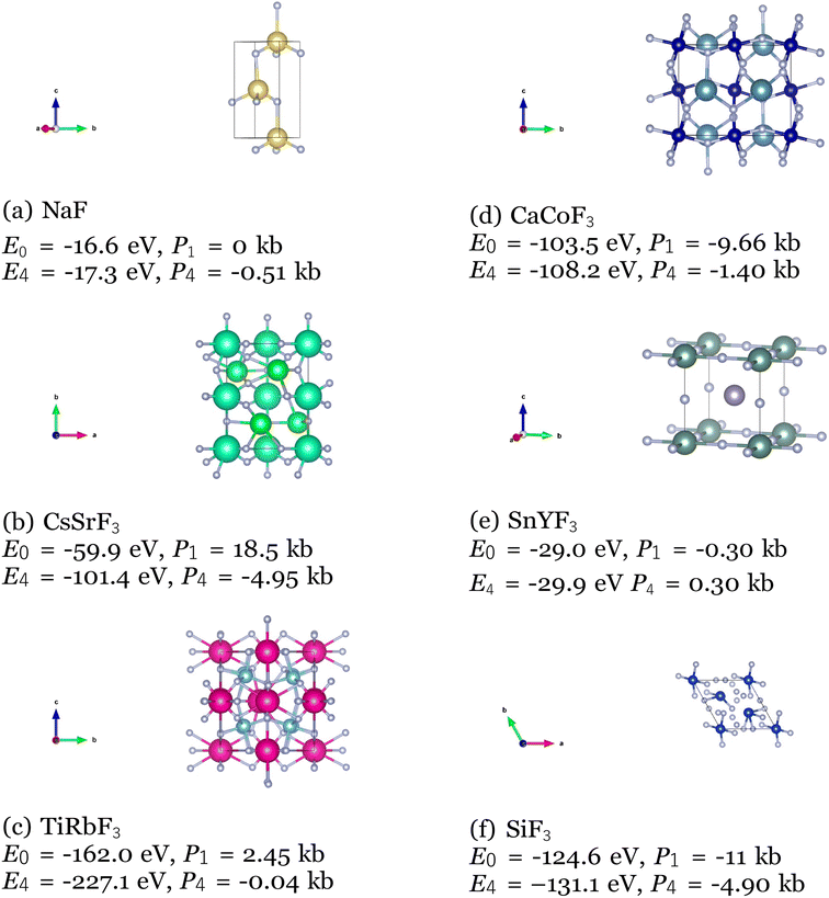Fig. 13 VASP calculated free energy and external pressure for 6 CIFs produced by the Diffusion Model.

As expected, all the free energies are lower and the external pressure values are closer to zero for the 4th relaxation, which indicates the VASP optimized the CIFs into even more stable structures. However, it is observed that the 6 CIFs exhibited low free energy and external pressure on the unit cell even from the pre-relaxation and 1st optimization. This is especially apparent for the NaF and SnYF₃ structures, which E₀ and E₄ are very close and the external pressure values after the 1st optimization are very close to 0 kb. These are strong indications of the stability of the produced CIFs.

7 Conclusion

In order to perform efficient material discovery via deep learning, it is important to find a representation that is capable of capturing all aspects of a given crystal structure. CrysTens encodes all of the pertinent values of a structure such as lattice parameters, lattice angles, and space group numbers as well as an interatomic component that is composed of a pairwise distance matrix and a dimensional graph for each dimension. The image-like nature of CrysTens allows for easy placement in image-generation models. The redundant aspects of CrysTens not only allow generative models many opportunities to mitigate noise when generating a crystal but it can also provide a way for measuring the performance of a given model. The variance of generated lattice parameters, lattice angles, space groups, and fractional coordinates is correlated with a model's ability to produce realistic and symmetrical crystals that have parameters similar to those found in the real distribution and even match the real distribution of CGCNN predicted values. We found that Vanilla GANs struggled in this space, often falling victim to training instability and mode collapse that ultimately lead to poor generated CIF quality. Many of these problems were rectified with the implementation of EMD and Wasserstein loss, creating a WGAN. However, although WGANs did not struggle with the same training instability and mode collapse that Vanilla GANs did, they failed to consistently produce symmetrical crystals. We found that Diffusion Models performed the best in this space. They performed the best in all of our metrics and consistently produced the most realistic-looking and symmetrical CIFs. The enhanced performance of Diffusion Models over GANs holds true in the image synthesis domain as well.⁵⁹ The use of Diffusion Models is extremely promising in the field of materials informatics and the improvement of such models may not only provide an efficient method of materials discovery but could revolutionize inverse design as well.

8 Future works

The performance of Diffusion Models in the materials discovery space creates a lot of opportunity for future works. The method of Diffusion Model generation we used in our work is known as unconditional generation. Conditional generation is the method that was responsible for all of the text-to-image breakthroughs that underpin powerful tools such as DallE-2 ⁵⁷ and Imagen.⁵⁸ It is possible to apply conditional generation to our work, as chemical formula-to-crystal generation. This could work by taking any chemical formula from PCD such as Ca₃AlB₂[OH]₁₅[H₂O]₁₁ and transforming it into a natural language analog such as “three calcium atoms, one aluminum atom, two boron atoms, fifteen hydroxide (one oxygen atom, one hydrogen atom) molecules, eleven water (one oxygen atom, two hydrogen atoms) molecules.” Extrapolated further into the realm of complex natural language we may be able to condition our Diffusion Models on statements such as “an oxide with offset layers of corner shared AlO6 octahedra with rare-earth filled interstitials,” which would allow for complex and diverse crystal generation. Another area worth exploring is classifier/regression guidance of Diffusion Models. Guidance allows Diffusion Models to take advantage of the outputs of a classifier or regressor to guide the reverse-diffusion process to ideal regression/classification outputs. This would make inverse design possible if the guiding model predicts material properties. These directions, along with increasing the complexity of our Diffusion Models, adding chemical descriptors as additional layers to CrysTens, and working towards an invariance satisfying version of CrysTens will be our next steps in this space.

9 Limitations

This work serves as a comparative analysis between GANs, WGANs, and Diffusion Models in crystal structure generation and illustrates the potential for Diffusion Models in the space of materials discovery. However, more analysis is needed to fully verify our Diffusion Model crystal generation methods. A comparison between our Diffusion Model methods and state-of-the-art material generators with CrysTens, as well as their native crystal representations, is required to wholly demonstrate the performance of our Diffusion Models. Additional rigorous DFT calculations of each of the produced crystals are needed as well. Furthermore, there are areas within the crystal generation process that still require (at times manual) tuning to correct errors that are accumulated during post-processing. This is especially true during the selection of K during K-means clustering for atomic numbers and atomic positions. This post-processing step damages the material generation pipeline as a whole because it forces crystals to conform to the given number of atomic numbers or positions even if the intended generated crystal contains different parameters. In order to fully understand the use of Diffusion Models in this space, it would be worthwhile to completely automate the material generation process.

Appendices

Appendix A: CIF details

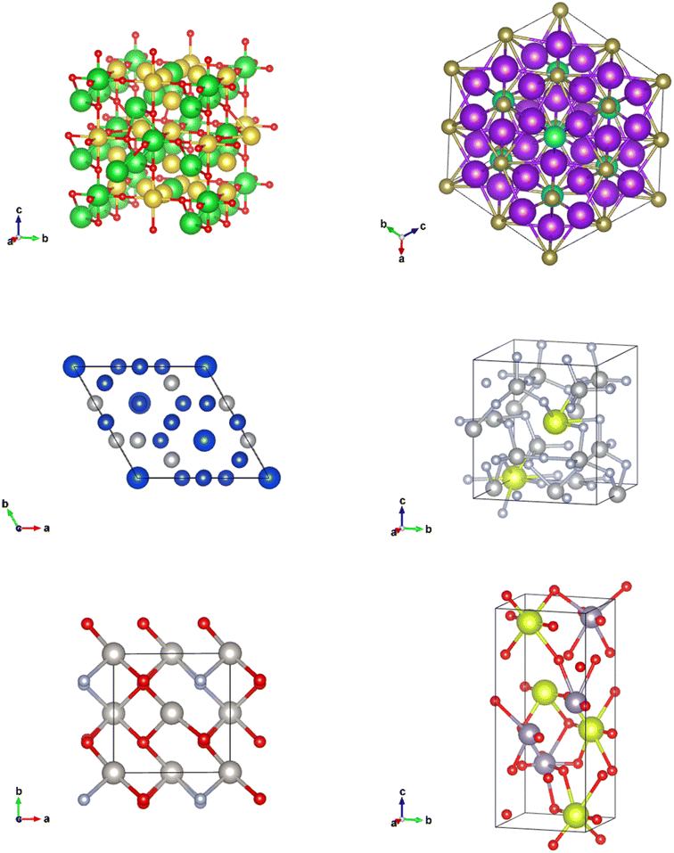
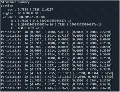
CIFs contain a simple body of text that entirely capture the fundamental chemistry and structure of a crystal structure. Software such as VESTA takes CIFs as input and outputs useful and aesthetically pleasing crystal visualizations that can aid in crystal chemistry research and education. In order for VESTA to create such visualizations, there are several key attributes that are needed within CIFs.⁶⁷ First, the lattice parameters and their angles with respect to one another are needed to establish the periodicity inherent in crystalline lattices. These lattice parameters also create the three-dimensional “bounding box” for the repeating unit cell and are generally represented with the variables a, b, and c with lattice angles α, β, and γ. Following the lattice information, the space group number is used to indicate which space group a particular crystal structure belongs to. The space group essentially encapsulates the symmetry properties of a given crystal structure or put more formally the space groups summarize the total number of three-dimensional patterns that are found in crystal structures.⁶⁸ The final information is the basis describing the arrangement of atoms associated with each lattice point. The basis allows us to distinguish different crystal structures having unique chemistries and atomic positions while retaining identical symmetry. The basis and the symmetry operations are combined to generate the exact atomic positions for all atoms within the unit cell.

With all of the crystal information organized within a CIF text file, VESTA is able to create visualizations as seen in Fig. 14 that assist materials scientists in determining the structural components of a given crystal. Pymatgen, a materials informatics Python library, was used to extract relevant information from each CIF during CrysTens construction using a Python programming interface and the Pymatgen Structure object (see Fig. 15).⁶⁹

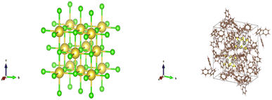Fig. 14 (left) A VESTA visualization of NaCl (right) a VESTA visualization of W₆S₈(PC₁₈H₁₅)₆(C₆H₆).⁶⁷

Fig. 15 A CIF represented as a Pymatgen structure object.

Appendix B: model details

All of the code used for training the models can be found at https://github.com/michaeldalverson/CrysTens.

B.1 Vanilla GAN. The Vanilla GAN was created using TensorFlow. It was trained for 100 epochs with a learning rate of 1 × 10⁻⁵ for both the discriminator and the generator. The latent dimension of the generator was 128. The loss function for the discriminator was binary cross-entropy. Both the discriminator and the generator contained a mixture of three-dimensional convolutional (transposed in the case of the generator) and dense layers. ReLU was used as the intermediate activation function in the generator and Leaky ReLU was used in the discriminator. Both neural networks used batch normalization.

B.2 Wasserstein GAN. The Wasserstein GAN was created using TensorFlow. It was trained for 100 epochs with a learning rate of 1 × 10⁻⁴ for both the critic and the generator. The loss function used was the Wasserstein loss. Gradient penalty was also used (to stabilize training) with a coefficient of λ = 10. Both the critic and the generator contained a mixture of three-dimensional convolutional (transposed in the case of the generator) and dense layers. The critic was trained 5 times as much as the generator. Leaky ReLU is used for both the critic and the discriminator and a mixture of layer normalization and batch normalization was used.

B.3 Diffusion model. The Diffusion Model was created using Imagen-Pytorch. The model was comprised of two Unets, which form the basis for the denoising diffusion probabilistic models.

Each Unet has 256 base channels. The first Unet created a “low-resolution” version of the CrysTens that was size 32 × 32 × 4. The second Unet, took the output of the first Unet and created the actual CrysTens of size 64 × 64 × 4. Each Unet was trained separately for 250 000 optimization steps with batch size 4. The original code is found at https://github.com/lucidrains/imagen-pytorch.

Data availability

The dataset used was Pearson's Crystal Data. All code and data can be found at https://github.com/michaeldalverson/CrysTens.

Author contributions

Michael D. Alverson: supervision, conceptualization, methodology, software, validation, formal analysis, investigation, visualization, writing – original draft & subsequent edits. Sterling G. Baird: methodology, software, writing – review & editing. Ryan Murdock: software, writing – review & editing. (Enoch) Sin-Hang Ho: VASP calculations, writing – editing. Jeremy Johnson: VASP calculations. Taylor D. Sparks: supervision, project administration, funding acquisition, conceptualization, resources, writing – review & editing.

Conflicts of interest

The authors declare no competing inter ests.

Acknowledgements

This work was supported by the National Science Foundation under CAREER Award 1651668. The Google TPU Research Cloud Program provided TPUs for training and testing.

References

1. A. Ludwig, Discovery of new materials using combinatorial synthesis and high-throughput characterization of thin-film materials libraries combined with computational methods, npj Comput. Mater., 2019, 5(70) DOI:10.1038/s41524-019-0205-0.
2. A. L. Greenaway, A. L. Loutris, K. N. Heinselman, C. L. Melamed, R. R. Schnepf and M. B. Tellekamp, et al., Combinatorial Synthesis of Magnesium Tin Nitride Semiconductors, J. Am. Chem. Soc., 2020, 142(18), 8421–8430,  DOI:10.1021/jacs.0c02092.
3. R. Bohacek, C. McMartin and W. Guida, The art and practice of structure- based drug design: a molecular modeling perspective, Med. Res. Rev., 1996, 16(1), 3–50,  DOI:10.1002/(SICI)1098-1128(199601)16:1<3::AID-MED1>3.0.CO;2-6.
4. Y. Dan, Y. Zhao, X. Li, S. Li, M. Hu and J. Hu, Generative Adversarial Net- works (GAN) Based Efficient Sampling of Chemical Composition Space for Inverse Design of Inorganic Materials, npj Comput. Mater., 2020, 6(1), 1–7.
5. V. Korolev, A. Mitrofanov, A. Eliseev and V. Tkachenko, Machine-Learning- Assisted Search for Functional Materials over Extended Chemical Space, Mater. Horiz., 2020, 7(10), 2710–2718.
6. Y. Sawada, K. Morikawa and M. Fujii, Study of Deep Generative Models for Inorganic Chemical Compositions, arXiv, 2019, preprint, arXiv:191011499,  DOI:10.48550/arXiv.1910.11499.
7. Q. Sun and S. H. Wei, Inverse Design of Stable Spinel Compounds with High Optical Absorption via Materials Genome Engineering, J. Mater. Chem. A, 2022, 10, 12503–12509.
8. L. Wei, Q. Li, Y. Song, S. Stefanov, E. Siriwardane, F. Chen, J. Hu, Crystal Transformer: Self-learning Neural Language Model for Generative and Tinkering Design of Materials, arXiv, 2022, preprint arXiv:2204.11953,  DOI:10.48550/arXiv.2204.11953.
9. R. Xin, E. M. D. Siriwardane, Y. Song, Y. Zhao, S. Y. Louis and A. Nasiri, et al., Active-Learning-Based Generative Design for the Discovery of Wide- Band-Gap Materials, J. Phys. Chem. C, 2021, 125(29), 16118–16128.
10. Z. Alperstein, A. Cherkasov and J. T. Rolfe, All SMILES Variational Autoencoder, arXiv, 2019, preprint, arXiv:1905.13343,  DOI:10.48550/arXiv.1905.13343.
11. N. Anand, R. Eguchi and P. S. Huang, Fully Differentiable Full-Atom Protein Backbone Generation, 2019.
12. N. Anand and P. Huang, Advances in Neural InformationProcessing Systems, in Generative modeling for protein struc-tures, ed. S. Bengio, H. Wallach, H. Larochelle, K. Grauman, N. Cesa-Bianchi and R. Garnett, Curran Associates, Inc, 2018, vol. 31, https://proceedings.neurips.cc/paper files/paper/2018/file/afa299a4d1d8c52e75dd8a24c3ce534f-Paper.pdf.
13. R. R. Eguchi, C. A. Choe and P. S. Huang, Ig-VAE: Generative Modeling of Protein Structure by Direct 3D Coordinate Generation, PLoS Comput. Biol., 2022, 18(6), 1–18.
14. N. C. Frey, V. Gadepally and B. Ramsundar, FastFlows: Flow-Based Models for Molecular Graph Generation, arXiv, 2022, preprint, arXiv:220112419,  DOI:10.48550/arXiv.2201.12419.
15. W. Gao, S. P. Mahajan, J. Sulam and J. J. Gray, Deep Learning in Protein Structural Modeling and Design, Patterns, 2020, 1(9), 100142.
16. M. Hoffmann and F. Noé, Generating Valid Euclidean Distance Matrices, arXiv, 2019, preprint, arXiv:1910.03131,  DOI:10.48550/arXiv.1910.03131.
17. H. Huang and X. Gong, A Review of Protein Inter-residue Distance Prediction, Curr. Bioinf., 2020, 15(8), 821–830.
18. D. Lemm, G. F. von Rudorff and O. A. von Lilienfeld, Machine Learning Based Energy-Free Structure Predictions of Molecules, Transition States, and Solids, Nat. Commun., 2021, 12(1), 4468.
19. Z. Li, S. P. Nguyen, D. Xu and Y. Shang, Protein Loop Modeling Using Deep Generative Adversarial Network, in 2017 IEEE 29th International Conference on Tools with Artificial Intelligence (ICTAI), IEEE, Boston, MA, 2017, pp. 1085–1091.
20. S. Ovchinnikov and P. S. Huang, Structure-Based Protein Design with Deep Learning, Curr. Opin. Chem. Biol., 2021, 65, 136–144.
21. B. Sanchez-Lengeling and A. Aspuru-Guzik, Inverse Molecular Design Using Machine Learning: Generative Models for Matter Engineering, Science, 2018, 361(6400), 360–365.
22. J. Westermayr, J. Gilkes, R. Barrett and R. J. Maurer, High-Throughput Property-Driven Generative Design of Functional Organic Molecules, Nat. Comput. Sci., 2023, 1–10.
23. F. Zhai and Q. Li, A Euclidean Distance Matrix Model for Protein Molecular Conformation, J. Glob. Optim., 2020, 76(4), 709–728.
24. R. Ahmad and W. Cai, Free Energy Calculation of Crystalline Solids Using Normalizing Flow, Modell. Simul. Mater. Sci. Eng., 2022, 30(6), 065007.
25. S. G. Baird, K. M. Jablonka, M. D. Alverson, H. M. Sayeed, M. F. Khan and C. Seegmiller, et al., Xtal2png: A Python Package for Representing Crystalstructure as PNG Files, J. Open Source Softw., 2022, 7(76), 4528.
26. G. Bergami, Gyankos/DGSOL, 2022, https://github.com/gyankos/DGSOL.
27. C. J. Court, B. Yildirim, A. Jain and J. M. Cole, 3-D Inorganic Crystal Structure Generation and Property Prediction via Representation Learning, J. Chem. Inf. Model., 2020, 60(10), 4518–4535.
28. S. Fredericks, K. Parrish, D. Sayre and Q. Zhu, PyXtal: A Python Library for Crystal Structure Generation and Symmetry Analysis, Comput. Phys. Commun., 2021, 261, 107810.
29. R. E. A. Goodall, A. S. Parackal, F. A. Faber, R. Armiento and A. A. Lee, Rapid Dis- covery of Stable Materials by Coordinate-Free Coarse Graining, Sci. Adv., 2022, 8(30), eabn4117.
30. S. Kim, J. Noh, G. H. Gu, A. Aspuru-Guzik and Y. Jung, Generative Adver- sarial Networks for Crystal Structure Prediction, ACS Cent. Sci., 2020, 6(8), 1412–1420.
31. I. H. Lee and K. J. Chang, Crystal Structure Prediction in a Continuous Repre- sentative Space, Comput. Mater. Sci., 2021, 194, 110436.
32. T. Long, N. M. Fortunato, I. Opahle, Y. Zhang, I. Samathrakis and C. Shen, et al., Constrained Crystals Deep Convolutional Generative Adversarial Net- work for the Inverse Design of Crystal Structures, npj Comput. Mater., 2021, 7(1), 66.
33. T. Long, Y. Zhang, N. M. Fortunato, C. Shen, M. Dai and H. Zhang, Inverse Design of Crystal Structures for Multicomponent Systems, Acta Mater., 2022, 231, 117898.
34. P. Lyngby and K. S. Thygesen, Data-Driven Discovery of 2D Materials by Deep Generative Models, npj Comput. Mater., 2022, 8(1), 232.
35. J. Noh, J. Kim, H. S. Stein, B. Sanchez-Lengeling, J. M. Gregoire and A. Aspuru- Guzik, et al., Inverse Design of Solid-State Materials via a Continuous Representation, Matter, 2019, 1(5), 1370–1384.
36. Z. Ren, S. I. P. Tian, J. Noh, F. Oviedo, G. Xing and J. Li, et al., An Invertible Crystallographic Representation for General Inverse Design of Inorganic Crystals with Targeted Properties, Matter, 2022, 5(1), 314–335.
37. H. Türk, E. Landini, C. Kunkel, J. T. Margraf and K. Reuter, Assessing Deep Generative Models in Chemical Composition Space, Chem. Mater., 2022, 34(21), 9455–9467.
38. P. Wirnsberger, G. Papamakarios, B. Ibarz, S. Racani`ere, A. J. Ballard and A. Pritzel, et al., Normalizing Flows for Atomic Solids, Mach. Learn.: Sci. Technol., 2022, 3(2), 025009.
39. T. Xie, X. Fu, O. E. Ganea, R. Barzilay and T. Jaakkola, Crystal Diffusion Variational Autoencoder for Periodic Material Generation, arXiv, 2021, preprint, arXiv:211006197,  DOI:10.48550/arXiv.2110.06197.
40. Y. Zhao, E. M. D. Siriwardane, Z. Wu, M. Hu, N. Fu and J. Hu, Physics Guided Generative Adversarial Networks for Generations of Crystal Materials with Symmetry Constraints, arXiv, 2022, preprint.
41. Z. Ren, S. I. P. Tian, J. Noh, F. Oviedo, G. Xing and J. Li, et al., An Invertible Crystallographic Representation for General Inverse Design of Inorganic Crystals with Targeted Properties, Matter, 2022, 5(1), 314–335.
42. Y. Zhao, M. Al-Fahdi, M. Hu, E. M. Siriwardane, Y. Song and A. Nasiri, et al., High-Throughput Discovery of Novel Cubic Crystal Materials Using Deep Generative Neural Networks, Advanced Science, 2021, 8(20), 2100566.
43. J. Köhler, M. Invernizzi, P. de Haan and F. Noé, Rigid Body Flows for Sampling Molecular Crystal Structures, arXiv, 2023, preprint, arXiv:2301.11355,  DOI:10.48550/arXiv.2301.11355.
44. Z. Ren, S. I. P Tian, J. Noh, F. Oviedo, G. Xing and J. Li, An invertible crys-tallographic representation for general inverse design of inorganic crystals with targeted properties, Matter, 2022, 5(1), 314–335 , https://www.sciencedirect.com/science/article/pii/S2590238521006251.
45. S. G. Baird, K. M. Jablonka, M. D. Alverson, H. M. Sayeed, M. F. Khan and C. Seegmiller, et al., xtal2png: A Python package for representing crystal structure as PNG files, J. Open Source Softw., 2022, 7(76), 4528,  DOI:10.21105/joss.04528.
46. Y. Zhao, M. Al-Fahdi, M. Hu, E. Siriwardane, Y. Song, A. Nasiri and J. Hu, et al., High-Throughput Discovery of Novel Cubic Crystal Materials Using Deep Generative Neural Networks, Adv. Sci., 2021, 8, 2100566.
47. E. Siriwardane, Y. Zhao, I. Perera and J. Hu, Generative Design of Stable Semiconductor Materials Using Deep Learning And DFT, npj Comput. Mater., 2022, 8(164).
48. A. S. Fuhr and B. G. Sumpter, Deep Generative Models for Materials Discov- ery and Machine Learning-Accelerated Innovation, Front. Mater., 2022, 9, 865270.
49. E. O. Pyzer-Knapp, J. W. Pitera and P. W. J. Staar, et al., Accelerating materials discovery using artificial intelligence, high performance computing and robotics, npj Comput. Mater., 2022, 8, 84.
50. J. Lim, S. Ryu and J. W. Kim, et al., Molecular generative model based on conditional variational autoencoder for de novo molecular design, J. Cheminf., 2018, 10(31) DOI:10.1186/s13321-018-0286-7.
51. S. Kim, J. Noh, G. H. Gu, A. Aspuru-Guzik and Y. Jung, Generative Adver- sarial Networks for Crystal Structure Prediction, ACS Cent. Sci., 2020, 6(8), 1412–1420,  DOI:10.1021/acscentsci.0c00426.
52. D. P. Kingma and M. Welling, Auto-encoding variational bayes, arXiv, 2013, preprint, arXiv:13126114,  DOI:10.48550/arXiv.1312.6114.
53. D. P. Kingma and M. Welling, et al., An introduction to variational autoen- coders, Found. Trends Mach. Learn., 2019, 12(4), 307–392.
54. F. Farnia and A. E. Ozdaglar, Do GANs always have Nash equilibria?, in ICML, 2020.
55. I. Goodfellow, J. Pouget-Abadie, M. Mirza, B. Xu, D. Warde-Farley and S. Ozair, et al., Generative adversarial networks, Commun. ACM, 2020, 63(11), 139–144.
56. M. Arjovsky, S. Chintala and L. Bottou, Wasserstein generative adversarial networks, in International conference on machine learning, PMLR, 2017, pp. 214–223.
57. A. Ramesh, P. Dhariwal, A. Nichol, C. Chu and M. Chen, Hierarchical text-conditional image generation with clip latents, arXiv, 2022, preprint, arXiv:220406125,  DOI:10.48550/arXiv.2204.06125.
58. C. Saharia, W. Chan, S. Saxena, L. Li, J. Whang, E. Denton, et al., Photorealistic Text-to-Image Diffusion Models with Deep Language Understanding, arXiv, 2022, preprint, arXiv:220511487,  DOI:10.48550/arXiv.2205.11487.
59. P. Dhariwal and A. Nichol, Diffusion models beat gans on image synthesis, Adv. Neural Inf. Process. Syst, 2021, 34, 8780–8794.
60. J. Ho, A. Jain and P. Abbeel, Denoising diffusion probabilistic models, Adv. Neural Inf. Process. Syst, 2020, 33, 6840–6851.
61. J. Sohl-Dickstein, E. Weiss, N. Maheswaranathan and S. Ganguli, Deep unsupervised learning using nonequilibrium thermodynamics, in, International Conference on Machine Learning, PMLR, 2015, pp. 2256–2265.
62. T. Xie and J. C. Grossman, Crystal graph convolutional neural networks for an accurate and interpretable prediction of material properties, Phys. Rev. Lett., 2018, 120(14), 145301.
63. C. Chen and S. P. Ong, A universal graph deep learning interatomic potential for the periodic table, Nat. Comput. Sci., 2022, 2(11), 718–728.
64. G. Kresse and D. Joubert, From ultrasoft pseudopotentials to the projector augmented-wave method, Phys. Rev. B: Condens. Matter Mater. Phys., 1999, 59, 1758–1775,  DOI:10.1103/PhysRevB.59.1758.
65. P. E. Blöchl, Projector augmented-wave method, Phys. Rev. B, 1994, 50, 17953–17979.
66. L. Schimka, R. Gaudoin, K. Jcv, M. Marsman and G. Kresse, Lattice con- stants and cohesive energies of alkali, alkaline-earth, and transition metals: Random phase approximation and density functional theory results, Phys. Rev. B: Condens. Matter Mater. Phys., 2013, 87, 214102.
67. K. Momma and F. Izumi, VESTA 3 for three-dimensional visualization of crys- tal, volumetric and morphology data, J. Appl. Crystallogr., 2011, 44(6), 1272–1276.
68. R. J. D. Tilley, Crystals and crystal structures, Wiley, 2020.
69. S. P. Ong, W. D. Richards, A. Jain, G. Hautier, M. Kocher and S. Cholia, et al., Python Materials Genomics (pymatgen): A robust, open-source python library for materials analysis, Comput. Mater. Sci., 2013, 68, 314–319 . Available from: https://www.sciencedirect.com/science/article/pii/S0927025612006295.

---