
Electrode informatics accelerated the optimization of key catalyst layer parameters in direct methanol fuel cells†
Lishou
Ban‡
a,
Danyang
Huang‡
a,
Yanyi
Liu‡
a,
Pengcheng
Liu
a,
Xihui
Bian
 b,
Kaili
Wang
c,
Yifan
Liu
*d,
Xijun
Liu
*e and
Jia
He
*a
b,
Kaili
Wang
c,
Yifan
Liu
*d,
Xijun
Liu
*e and
Jia
He
*a
aSchool of Chemistry and Chemical Engineering, Institute for New Energy Materials & Low-Carbon Technologies, School of Materials Science and Engineering, Tianjin University of Technology, Tianjin 300384, China. E-mail: hejia1225@126.com
bState Key Laboratory of Separation Membranes and Membrane Processes, School of Chemical Engineering and Technology, Tiangong University, Tianjin 300387, China
cSchool of Chemistry, Chemical Engineering and Environmental Engineering, Weifang University, Weifang 261061, China
dSuzhou Laboratory, Suzhou 215100, China. E-mail: sparkle06@163.com
eMOE Key Laboratory of New Processing Technology for Nonferrous Metals and Materials, Guangxi Key Laboratory of Processing for Non-ferrous Metals and Featured Materials, School of Resources, Environment and Materials, Guangxi University, Nanning, 530004 Guangxi, China. E-mail: xjliu@gxu.edu.cn
First published on 11th November 2024
Abstract
As the core component of direct methanol fuel cells, the catalyst layer plays the key role as a species, proton and electron transport channel. However, due to the complexity of the system, optimizing its performance involves a large number of experiments and high costs. In this study, finite element simulation combined with machine learning model was constructed to accelerate power density prediction and evaluate the influence of catalyst layer parameters on the maximum power density of direct methanol fuel cells. We built a fuel cell simulation model corresponding to different parameters, obtaining a database of more than 200 sets of 19 eigenvalues, and then used different machine learning models for training and prediction. Finally, three tree-integration methods were selected to rank the importance of 19 characteristic parameters. In addition, we performed a high-throughput screening of 200![[thin space (1/6-em)]](https://www.rsc.org/images/entities/char_2009.gif) 000 different parameter combinations based on sequential model-based algorithm configuration. We selected the top 10 parameter combinations with high expected improvement scores and employed them into a numerical simulation model. The results show that a majority of the polarization curves obtained from the top combinations exceed the maximum power density of the original database. This method greatly saves the time of collecting fuel cell data for experiments and speeds up the parameter optimization process.
000 different parameter combinations based on sequential model-based algorithm configuration. We selected the top 10 parameter combinations with high expected improvement scores and employed them into a numerical simulation model. The results show that a majority of the polarization curves obtained from the top combinations exceed the maximum power density of the original database. This method greatly saves the time of collecting fuel cell data for experiments and speeds up the parameter optimization process.
1 Introduction
As a device that converts chemical energy directly into electrical energy, fuel cells have the advantages of high efficiency and environmental protection.1–4 Among fuel cells, hydrogen-related proton-exchange membrane fuel cell is one of the important types.5 However, before the application of hydrogen fuel cells, problems related to hydrogen production, hydrogen storage, and hydrogen transportation need to be solved, which brings development opportunities for methanol fuel cells.6 Among them, direct methanol fuel cell (DMFC) has the characteristics of direct fuel injection into the stack, simple cell structure, and high cell energy density.7–10 In the membrane electrode assembly, the catalyst layer (CL) is the core component, and its performance has a great influence on the output power density of the electrode in DMFC. Therefore, optimizing the CL design parameters of DMFC is crucial to improve its power density and overall performance.11,12 At the physical level, factors such as catalyst loading,21 ionomer ratio,22 and humidity23 play key roles in fuel cell performance. It is also of great significance to study the parameters that affect the operation of DMFC for the efficient and sustainable operation of DMFC.13–20 Operating parameters such as temperature, backpressure, and reactant flow rates further increase the complexity of the parameter space. This means that the development of efficient electrode designs for DMFCs needs the integration of multiple aspects of effort. Experiments involving too many factors can also lead to confounding of the test criteria. Therefore, it is extremely difficult to draw general rules from these complex data. To address the above challenge, a suitable tool is required to draw effective conclusions from a large number of interrelated and mutually affecting factors to guide the design of electrodes for DMFC.Numerical modelling has played a crucial role in recent research related to DMFCs as it allows for the modification of relevant parameters to understand and predict the behaviour and performance of fuel cells. A variety of DMFC models has been developed to better understand the performance of DMFC under different conditions. For example, Yang et al.24 combined theoretical and empirical models to establish a semi-empirical model that describes the relationship between the operating parameters, such as temperature, methanol concentration, methanol and air flow rates, and the performance of DMFCs. The model is sufficiently accurate to estimate the system performance and is suitable to investigate the DMFC degradation mechanism. Yu et al.25 established a single-phase three-dimensional computational fluid dynamics (CFD) model to study the effects of channel geometry and operating parameters on DMFC performance. In addition, the model also has the potential for geometric parameter optimization design and operational parameter optimization control to develop DMFC systems. Tafaoli-Masoule26 proposed a quasi-two-dimensional isothermal model for DMFCs to obtain the power exponent as the fitness function of a genetic algorithm and used genetic algorithms to determine the optimal parameters for maximizing the power of a single-cell DMFC. The optimal values of the DMFC cell temperature, anode and cathode pressure and channel height were determined to be 130 °C, 2.5 bar, 5 bar and 1 mm, respectively. Lee et al.27 proposed an active DMFC system model that combines a one-dimensional DMFC stack model with major system components. The effects of DMFC operating parameters and thermal management were analysed through numerical modelling and simulations. The model determined that 0.6 M is the optimal methanol feed concentration to achieve the highest stack performance and also revealed the influence of ambient temperature and anode inlet temperature. Jiang et al.28 proposed a two-phase two-dimensional model for DMFC with an ordered structure cathode CL, considering water accumulation around the cylindrical carbon nanowires in oxygen radial transport. The results show that DMFC with ordered electrodes can produce better cell performance. The above research results indicate that the application of numerical simulation in DMFCs has been very extensive, and it can gradually reveal the influence of many complex physical fields on the performance of DMFCs and provide guidance for the design of electrodes. However, numerical simulation also has the disadvantages of large amount of calculation, long time-consuming, and high computational cost. Moreover, if researchers want to study the relationship between different parameters and optimize a series of parameters at the same time, numerical simulation is particularly difficult.
Machine learning (ML), as a data-driven technique based on limited data and model training, has the potential to solve this problem. ML can obtain a certain data fitting model on the basis of existing data, revealing the hidden rules behind the input characteristics and output of the target system, such as image recognition driven by deep learning network,29 personal recognition,30 and automatic driving.31 The complexity of DMFC also provides a suitable place for data-driven modelling. At present, the M model has been successfully applied to performance prediction, aging prediction and fault diagnosis of fuel cells and has obtained good accuracy in solving nonlinear problems. Combined with the optimization algorithm, the ML model can further optimize the design and operating parameters to achieve multiple optimization goals with good accuracy and efficiency.32–39 For example, Liu et al.40 designed an AI-based NPME auxiliary model for proton-exchange membrane fuel cell, which can well predict and analyse the maximum output power density and polarization curve by training with real experimental data in the literature. Ding et al.41 trained nine different ML algorithms on experimental datasets in the laboratory to accurately predict performance and Pt utilization (Max R2 = 0.973/0.968). The black-box interpretation method is applied to provide reliable insights into the optimal synthesis conditions from both qualitative and quantitative perspectives. Under the guidance of ML results, the ionomer/catalyst ratio, water content, organic solvent, catalyst load, stirring mode, solid content and ultrasonic spraying flow rate were optimized. The utilization rate of platinum is 0.147 g Pt kW−1 and the power density is 1.02 W cm−2. The above research work shows that compared with numerical simulation technology, data-driven technology occupies much less time and computational resources and has a high degree of versatility. However, due to the complex structure and spatial characteristics of DMFC system electrodes, it is challenging to build a directly coupled electrode model by numerical simulation. Combining ML with numerical modelling is a promising method to improve the model accuracy and speed up the simulation process. This combination helps to better understand and predict the behaviour of complex systems, providing stronger support for scientific research and engineering practice.
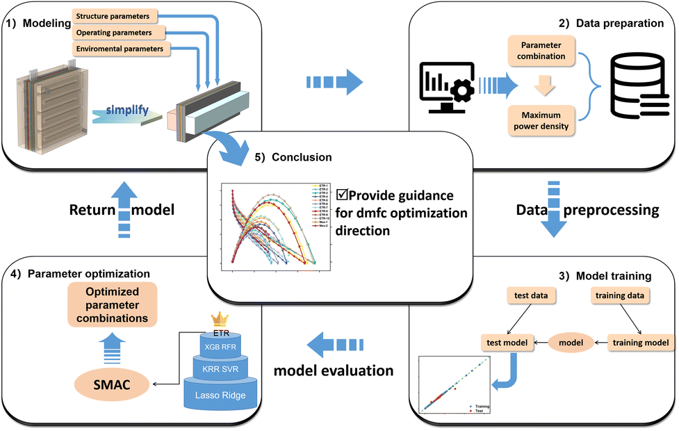
In this paper, a 3D MEA model of DMFC is firstly established, and the influence of key parameters affecting CL on DMFC performance is discussed. The model consists of an anode/cathode flow channel, an anode/cathode diffusion layer, an anode/cathode CL, and a proton-exchange membrane that work together to achieve efficient energy conversion in DMFC. The model follows the mass conservation equation, momentum conservation equation and charge conservation equation, and the established model can clearly show the mass transfer process of the inlet and outlet flow channels and membrane electrodes of the fuel cell. Then, the different parameters of CL are calculated as input parameters, and the power density is used as the output parameter to establish the database. Regression models were built using 7 different ML algorithms to assess the importance of each parameter. Finally, precise combined data for predicting the output performance were obtained and calculated using the simulation model to obtain the I–V polarization curve and maximum power density, which were then compared with the data in the database. Scheme 1 describes the main aspects of the work. The results show that more than half of the polarization curves obtained from the top 10 parameter combinations with expected improvement (EI) score exceed the maximum power density of the original data. Therefore, the combination of numerical simulation and machine learning can greatly save the time of collecting fuel cell data for experiments and accelerate the parameter optimization process.
 | ||
| Scheme 1 Simulation and data dual-drive parameter optimization process. | ||
2 Methods
2.1 DMFC numerical model
(1) DMFC operates under steady-state conditions.
(2) The cross methanol from anode to cathode is completely oxidized by oxygen in the cathode CL.
(3) GDL, CL and membrane have isotropic permeability and effective porosity.
(4) The electrochemical reaction is complete, with only CO2 and H2O being produced.
(5) The flow is laminar, both fully developed and incompressible.
(6) A mixture of reaction gases is considered ideal.
(7) The process is isothermal.
(8) Gravity effects are ignored.
(9) The catalytic layer and diffusion layer of the anode and the cathode have the same diffusivity and other characteristic parameters. The effects of the resulting carbon dioxide are ignored; the transfer of heat throughout the process is ignored.
(10) All physical properties are assumed to be immutable.
(11) The contact resistance between layers is ignored.
2.1.2.1 Electrochemical kinetics. The reaction mechanism of the electrooxidation reaction of methanol at the anode and the electroreduction reaction of oxygen at the cathode is relatively complex, and its electrochemical reaction rate can be described by the Butler–Volmer rate expression,42 which can be simplified to obtain a Tafel type equation of methanol concentration, as shown below.
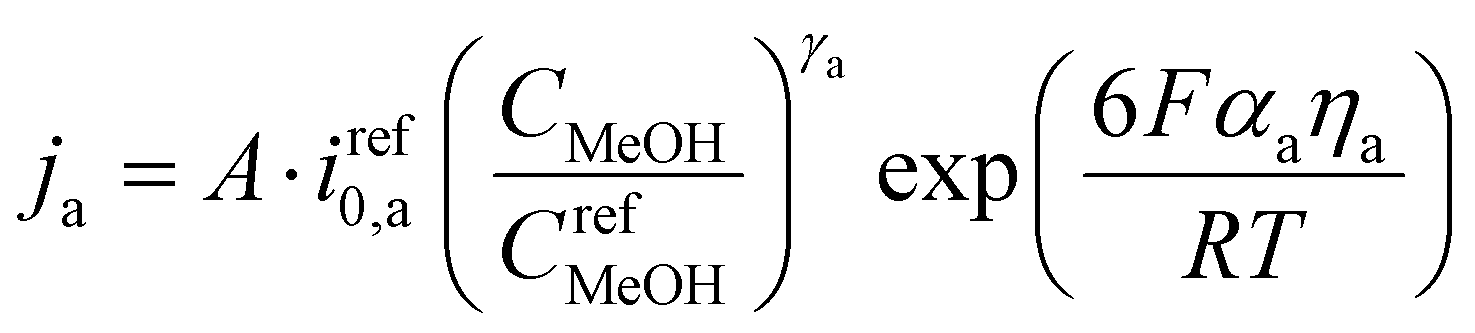 | (1) |
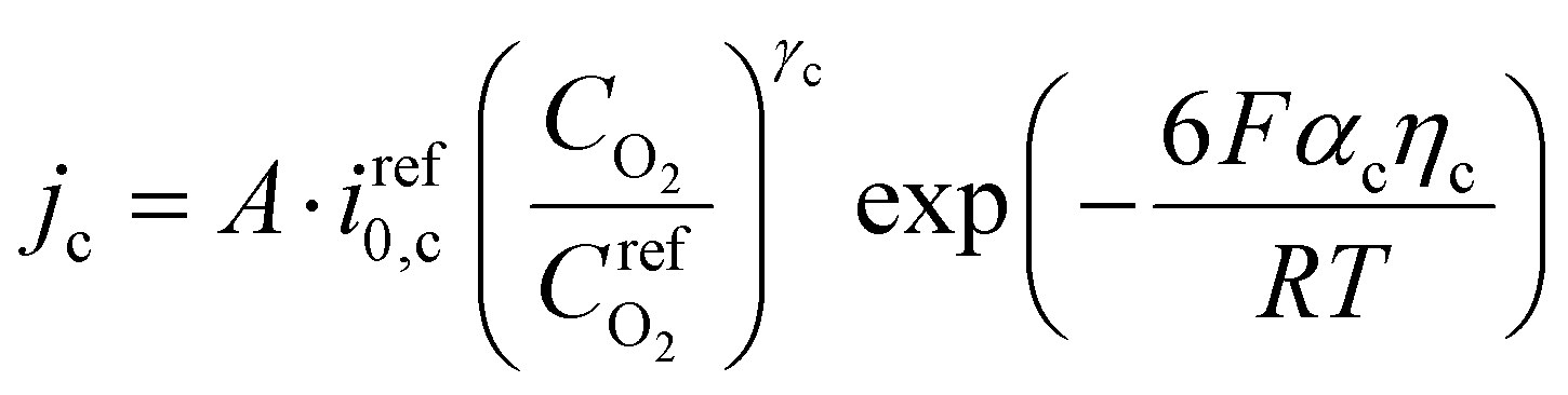 | (2) |
The overpotential ηa and ηc for the anode and cathode at any location within the CL is defined as follows.
| ηa = ϕs − ϕm − Eaeq | (3) |
| ηc = ϕs − ϕm − Eceq | (4) |
2.1.2.2 Ohm's law. The transport of protons and electrons in the membrane electrode assembly follows Ohm's law. The general equation form can be given by the following formula.
| ∇·(−σeffm∇ϕm) = im | (5) |
| ∇·(−σeffs∇ϕs) = is | (6) |
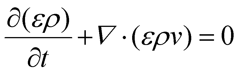
2.1.3.1 Mass conservation equation. The mass conservation equation (continuity equation) basically requires that the change in mass per unit volume in a given time must be equal to the sum of all substances entering or leaving that volume. The mass conservation equation is
 | (7) |
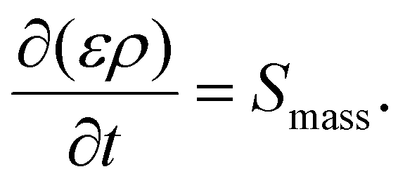 | (8) |
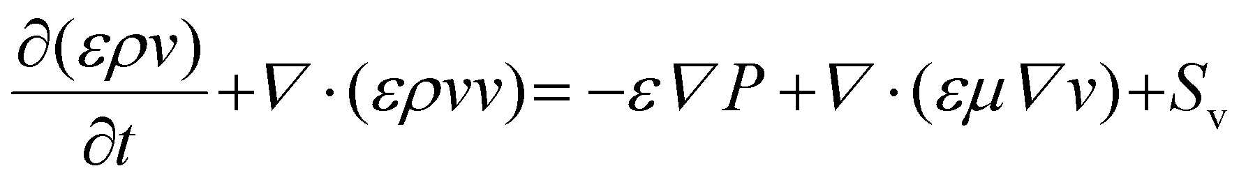
2.1.3.2 Charge conservation equation. Momentum transfer can be described by the Navier–Stokes equation.43 The flow of methanol in the flow channel is considered laminar and continuous, and the momentum of the flow comes from the pressure difference ∇P.
 | (9) |
Since the steady-state system is used, it will not change with time, and the above formula can be simplified as follows.
| ∇·(ερvv) = −ε∇P + ∇·(εμ∇v) + Sv | (10) |
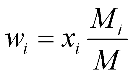
2.1.3.3 Species conservation equation. The transport of substances through the anode and cathode is controlled by a combination of diffusion and convection.
| ρ(u·∇)wi = ρDeffi∇2wi + Si | (11) |
 | (12) |
2.1.3.4 Membrane permeability equation. The transfer of methanol through Nafion membranes occurs through diffusion and electroosmosis. Since the pressure difference between the two sides of the membrane is negligible, methanol permeated from the anode passes through the membrane to the cathode CL and is then completely consumed, resulting in a parasitic current; thus, the methanol permeation equivalent current density (Ixover) is determined by the following formula.
| Ixover = 6FNMMeOH | (13) |
The cross flux of methanol is calculated by eqn (2)–(13).
 | (14) |
2.2 Machine learning
In this study, we applied seven different ML algorithms to process the data. In order to improve the fitness of ML model and database, we correctly processed and evaluated the performance of seven model algorithms based on Root Mean Square Error (RMSE). In performance prediction, we chose three algorithms with the smallest RMSE, namely, ETR, RFR and XGB for performance prediction. Two of these methods involve linear regression methods (Lasso, Ridge), and five involve nonlinear regression methods (including two kernel methods (KRR, SVR) and three tree integration methods (RFR, XGB, and ETR)). This set of ML models covers a wide range of model types that can reveal relevant aspects of different data.The quantitative evaluation of prediction accuracy is based on the root-mean-square error calculated by 10-fold cross-validation, which is the most commonly used method in prediction error estimation.44–48 Ten-fold cross-validation is an ML cross-validation method that divides the data set into 10 subsets, each of which is used to train the model and then combines the results of these 10 subsets to evaluate the performance of the model. The main advantage of ten-fold cross-validation is that the performance of the model can be evaluated in a shorter period of time as it only needs to evaluate the results of 10 subsets rather than the entire data set. Furthermore, ten-fold cross-validation can also help find potential flaws in the model as it can find problems in the model in a shorter period of time. Herein, we used ten-fold cross-validation to evaluate the predictive performance of the model.
To evaluate the input feature variables that contribute the most to the prediction of the target of interest, the feature importance score provided by the tree-integration method was used.49,50 The importance score, which can be of many types, is usually calculated as a weighted average of the squared error improvement attributed to a single feature variable and represents the relative importance of each feature variable relative to the predictability of the target variable. The input feature variables are rarely equally correlated and usually only a few have a significant effect on the predicted target variable.
We then extend this further to predict the entire output I–V polarization curve of the DMFC. An SBO (surrogate-based optimization) strategy based on the sequential model-based algorithm configuration (SMAC) program was developed and evaluated using expected improvement (EI). EI calculates the expected improvement value for each candidate configuration based on the prediction results and uncertainty of the current surrogate model. This value typically considers two factors: the performance prediction (mean) and the uncertainty (standard deviation) of the candidate configuration. By comparing the EI values of different candidate configurations, the SBO strategy can select the most promising one.
All of the ML computational work was done by writing code in the Python 3.7 environment. All ML models make extensive use of the Scikit-learn package (version 0.24.1) and XGB uses the XGBoost package (version 1.3.3).
3. Results and discussion
3.1 Grid independence verification
In this study, COMSOL Multiphysics was used as the finite element solver. In order to simplify the model and improve the computing efficiency, we cut out a part of the structure of the DMFC and constructed a model including the flow channel of the positive (negative) electrode, the diffusion layer of the positive/negative electrode, the catalytic layer of the positive/negative electrode, and the proton exchange membrane. After entering all the necessary equations (secondary current distribution, transport of dilute matter, transport of dense matter, Brinkman equations, phase transport of porous media and electrochemical relations), a grid was generated for the geometry using the software's built-in module. Fig. 1 shows the DMFC model after grid division. The structured hexahedral grid was generated by scanning and mapping methods. To build the grid, the maximum cell size was set to 1 mm and the maximum element growth rate was set to 1.5. Grid independence verification can determine the balance between calculation speed and calculation accuracy.51–53 Fig. S1† shows the results of the grid independence verification. Considering the cost and time, the number of mesh encryption layers is selected as the norm after balancing the accuracy and calculation. | ||
| Fig. 1 3D geometric model of DMFC. | ||
3.2 DMFC simulation model
The geometric parameters, physical and chemical properties and operating conditions used in this modeling work are shown in Table S2.† The operating temperature was maintained at 333.15 K, the methanol concentration was 1 M, and the flow rates of methanol and air were 6 mL min−1 and 600 sccm, respectively. More details corresponding to the literature simulation can be found in the references.54 It can be seen from Fig. 2(a) that the simulated polarization curve is consistent with the simulation results in the literature. The polarization curve of the simulated 1 M methanol solution was compared with the calculated polarization curve obtained from the experimental data obtained in the research group's literature,55 as shown in Fig. 2(b). In the experiment, the materials used in the fuel cell included Nafion 115 for the membrane and Pt–Ru with a loading of 0.2 mg cm−2 for the anode CL. Methanol solution and air flow were supplied to the anode and cathode at 80 °C, respectively. Anode inlet flow rate Qa was set at 2 mL min−1, and cathode inlet flow rate Qc was set at 100 sccm. The simulation results are in good agreement with the experimental values of the research group, which proves that the three-dimensional multi-phase model is accurate, reliable and reasonable.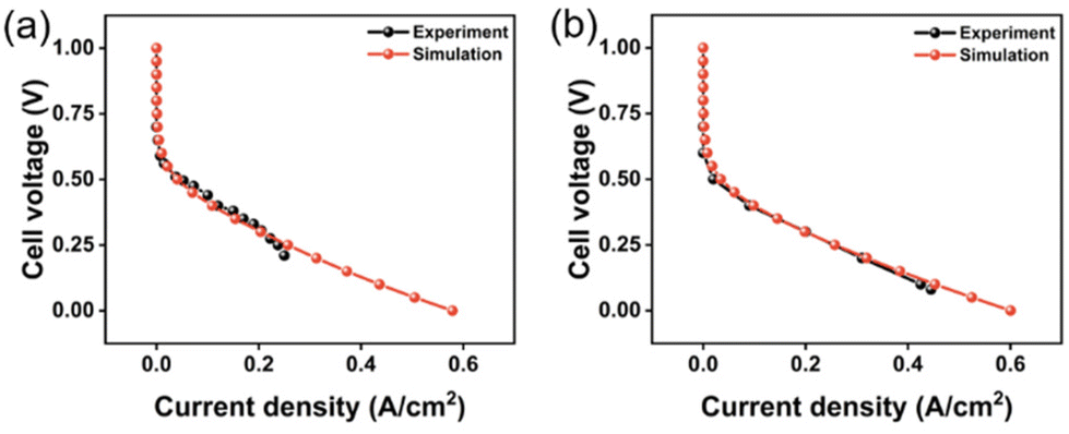 | ||
| Fig. 2 (a) Comparison of polarization curve with polarization curve obtained from simulation literature parameters54 and (b) Comparison of polarization curve with polarization curve obtained from experimental literature parameters.55 | ||
For a cell voltage of 0.25 V (voltage at maximum power density), the distribution of methanol concentration, CO2 concentration, oxygen concentration and cathode water concentration is shown in Fig. S2.† From the distribution of substance concentrations in the figure, it can be seen that fluid flow has been fully developed in the channel. In Fig. S2(a–d),† methanol concentration decreases along the length direction (y positive direction) and thickness direction (z positive direction) as methanol is transmitted through the flow channel to CL, and methanol just participates in the reaction at the entrance; thus, less methanol is consumed and the current density is lower. With the diffusion of methanol, the more intense the reaction, the greater the reduction of methanol concentration. Methanol concentration ranges from 1000 to 997.75 mol m−3. As a product, the concentration distribution of CO2 is completely opposite to that of methanol, increasing from 0.0001 to 2.2485 mol m−3. This suggests that the more the methanol diffuses, the more intense the reaction in the middle. The concentration distribution of oxygen and water corresponds to the concentration distribution of methanol and CO2, respectively. Oxygen and protons in the cathode CL generate water, oxygen consumption, and liquid water. The distribution of water is mainly concentrated in the cathode CL and GDL, which makes it easy to accumulate water, and the phenomenon of “waterflooding” occurs.56 The methanol permeated from the anode reaches the cathode CL, where it is then completely consumed, and the resulting current indicates the amount of methanol permeated. The unreacted methanol is transported to the cathode by diffusion and electroosmosis driving forces. In Fig. S2(e),† it can be seen that the methanol flux per unit time in the cathode CL is very low, indicating a very low cross-current density. The saturation distribution of the cathode liquid is shown in Fig. S2(f).† There is a clear dividing line between the flow channel and the cathode GDL interface. However, the amount of change is small because the change in the saturation of liquid water in the cathode can be considered negligible.
3.3 The polarization curve obtained by CL key parameter screening
The polarization curve serves as a tool to describe the performance and performance losses of fuel cells under various operating conditions. The polarization curve can be divided into three regions: activation polarization, ohmic polarization, and mass transport polarization. Among them, activation polarization is caused by the slow reaction on the electrode surface. Ohmic voltage drop arises from the resistance to ion transport in the anode, cathode, electrolyte, and other interconnections. Mass transport polarization results from the existence of certain resistance in the mutual transport of fuel and oxygen during electrode reactions. By optimizing the parameters to improve these three polarization regions, the performance of fuel cells can be enhanced.Therefore, we selected temperature, anode/cathode CLs thickness, porosity, Nafion content, anode inlet flow rate, cathode inlet flow rate, anode catalytic layer permeability, cathode catalytic layer permeability, anode methanol inlet concentration, anode specific surface area, cathode specific surface area, reference pressure, anode/cathode electron conductivity, anode/cathode proton conductivity, reference methanol concentration, reference oxygen concentration, a total of 19 parameters that may affect the polarization phenomenon, as input characteristics. For each parameter, we tried to choose the one with the lowest correlation. The power density is considered to be the output.57,58Table 1 lists the input parameters and their value ranges. Then, we built a database of fuel cells.
| Variables | Expression | Range |
|---|---|---|
| Temperature (K) | T (K) | 288.15–378.15 |
| Thickness of anode CL (m) | H_electrode_an (m) | (5 × 10⁻⁷)–(7.5 × 10⁻⁵) |
| Thickness of cathode CL (m) | H_electrode_ca (m) | (5 × 10⁻⁷)–(7.5 × 10⁻⁵) |
| Porosity of anode CL (%) | eps_CL_p_a (%) | 10–90 |
| Porosity of cathode CL (%) | eps_CL_p_c (%) | 10–90 |
| Nafion content of anode CL (%) | eps_CL_l_a (%) | 5–60 |
| Nafion content of cathode CL (%) | eps_CL_l_c (%) | 5–60 |
| Anode inlet flow rate (m s−1) | U_in_an (m s−1) | 0.01–2 |
| Cathode inlet flow rate (m s−1) | U_in_ca (m s−1) | 0.1–8 |
| Permeability of anode CL (m2) | kappa_CL_an (m2) | (1 × 10⁻¹⁵)–(5 × 10⁻¹¹) |
| Permeability of cathode CL (m2) | kappa_CL_ca (m2) | (1 × 10⁻¹⁵)–(5 × 10⁻¹¹) |
| Anode methanol inlet concentration (M) | C MeOH_in (M) | 0.1–15 |
| Anode specific surface area (1 m−1) | Av_an (1 m−1) | (1 × 10⁴)–(1 × 10⁷) |
| Cathode specific surface area (1 m−1) | Av_ca (1 m−1) | (1 × 10⁴)–(1 × 10⁷) |
| Reference pressure (atm) | p_ref (atm) | 0.1–8 |
| Positive cathode electron conductivity (S m−1) | sigma_CL_s (S m−1) | 10–1000 |
| Positive cathode proton conductivity (S m−1) | sigma_CL_i (S m−1) | 1–19 |
| Reference methanol concentration (mol m−3) | c MeOH_ref (mol m−3) | 10–500 |
| Reference oxygen concentration (mol m−3) | c O2_ref (mol m−3) | 5–50 |
 | (15) |
Therefore, the ECSA can be changed by controlling the Av when the Pt loading volume is unchanged.
Fig. 3 shows Av changes for different anode and cathode CLs. As can be seen from the polarization curve in Fig. 3(a), anode Av can cause large ohmic polarization and concentration polarization but has little effect on activation polarization. The cell performance increases as the Av range increases from 1 × 10⁴ to 1 × 10⁷, and the increase trend is more gradual at 3 × 10⁵. The final Av is 2.3 times larger than the previous one, while the maximum power density is only 16% better. It may be due to the failure of the reaction products to leave the catalyst surface, which leads to the mass transfer obstruction, thus limiting the performance improvement. As can be seen from the polarization curve in Fig. 3(b), the change in Av has a great influence on activation polarization and ohmic polarization. As the current density increases, the impact of Av on cell performance gradually increases. More and more active sites on the cathode are involved in the reaction, which is conducive to the oxygen reduction reaction. In Fig. 3(c), when the Av of the anode and cathode CLs is changed at the same time, the cell performance improvement is not obvious when the anode Av or cathode Av is increased separately because the anode Av and cathode Av are increased at the same time; thus, the reaction products of the cathode and anode cannot be transmitted out in time, which affects the cell performance. Therefore, when optimizing the electrochemical system, it is necessary to comprehensively consider the synergistic effect of the anode and cathode to ensure the effective transmission of reaction products to achieve the best performance.
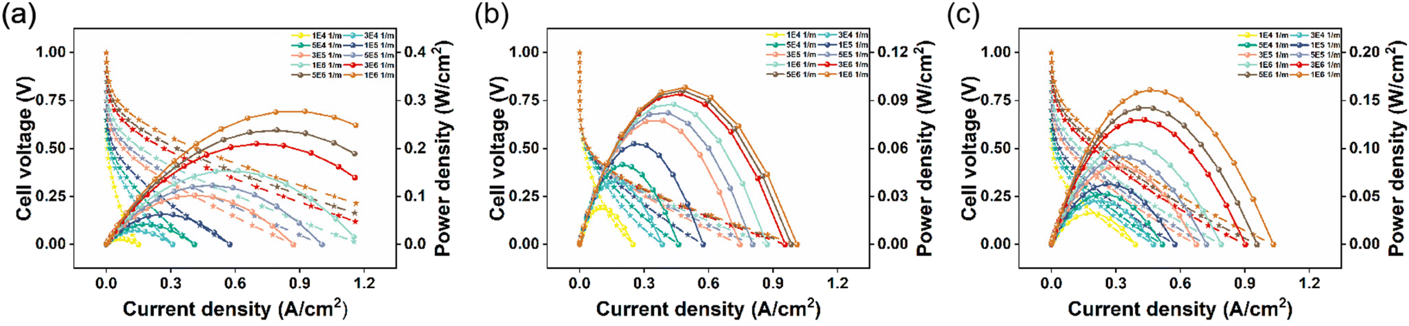 | ||
| Fig. 3 Polarization curve obtained by changing the active specific surface area (Av): (a) anode CL; (b) cathode CL; (c) the anode and cathode CLs. | ||
 | ||
| Fig. 4 Polarization curve obtained by changing the CL thickness: (a) change of anode CL thickness; (b) change of cathode CL thickness; (c) change of anode and cathode CLs thickness. | ||
Fig. S5(b)† shows the polarization curve under different working pressures from 0.1 to 8 atm. In the small current range, the effect of increasing pressure on the output performance of the fuel cell is not significant, while in the large current range, the effect of increasing pressure on the output performance is gradually improved. The higher the pressure, the better the output performance of the fuel cell system. However, the specific working pressure that can be achieved depends on the maximum pressure that the stack and the membrane electrode can withstand. In addition, in real situations, high pressure can lead to an increase in the parasitic power of related equipment, which can offset some of the performance improvements caused by increased pressure, thereby reducing the net power density of fuel cells. When designing and optimizing fuel cell systems, it is necessary to comprehensively consider factors such as performance under different pressures, system complexity, and cost to achieve optimal power density and performance.
Fig. S6(a)† shows the polarization curves for different electron conductivities of the positive cathode catalytic layer. In order to ensure that the catalytic layer and the diffusion layer have good electrical conductivity and ensure electron transmission, the electronic conductivity needs to be hundreds or more. In this paper, the cell performance is calculated in the range of 10–1000 S m−1, and it is found that the change in the electronic conductivity has little effect on the cell performance. This is because the electronic conduction path has been effectively established at the three-phase interface. However, this does not mean that electronic conductivity can be completely ignored. In practical applications, if the electronic conductivity is insufficient, it may lead to an increase in internal resistance of the fuel cell, thereby affecting the output performance and efficiency of the fuel cell.
Generally speaking, the conductivity of the membrane is below 20 S m−1, and the main range of the effective proton conductivity discussed here is 1–19 S m−1. The proton conductivity is closely related to the water content of the Nafion membrane, which is related to the proton transport process and mode. The conductivity of the proton-exchange membrane plays an important role in charge transport loss. As shown in Fig. S6(b),† in the low current density region, the efficiency of the fuel cell is mainly affected by activation loss; thus, it is insensitive to effective proton conductivity and does not show significant changes. At medium to high current densities, Ohmic loss becomes the main component of fuel cell performance loss. The improvement of proton conductivity helps to reduce Ohmic losses. However, as proton conductivity increases, the rate of improvement in fuel cell performance will gradually slow down, and there may even be a convergence trend. This is because when the proton conductivity reaches a certain level, the efficiency of proton transport in the membrane is close to its limit, and a further improvement of proton conductivity will have limited impact on the fuel cell performance.
This conclusion can be explained from the perspective of electrochemical kinetics. A smaller reference concentration means that the concentration gradient of reactants on the electrode surface is larger, thereby promoting the diffusion of reactants and increasing the reaction rate. Therefore, in fuel cells, optimizing the supply and concentration distribution of methanol and oxygen can potentially improve the exchange current density, thereby enhancing the performance of the cell.
Finally, we organized the amplitude range of the maximum power density of the direct methanol fuel cell simulation model after adjusting each parameter to understand the importance of each parameter on the maximum power density. The results are shown in Fig. S9,† which displays the top six parameters in terms of maximum power density amplitude ranking.
3.4 Model- and data hybrid-driven prediction
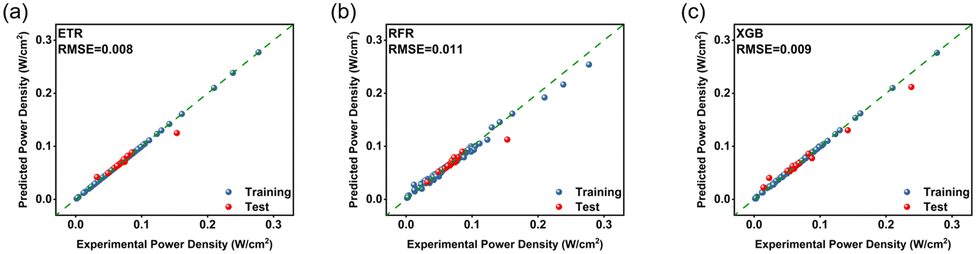 | ||
| Fig. 5 Data training test (10-fold cross-validation) error graph of three algorithms based on the tree-integration method. (a) ETR; (b) RFR; (c) XGB. Training data (blue), test data (red). | ||
We chose root mean square error (RMSE) and standard deviation (STD) to evaluate the prediction accuracy of the algorithm. Table 2 shows the RMSE and STD of the data training test obtained by seven different algorithms. Nonlinear methods (KRR, SVR, RFR, XGB, ETR) perform better than linear methods (Lasso, Ridge), and in particular, tree-integration methods (RFR, XGB, and ETR) have smaller training and test errors because they can capture nonlinear relationships in data, have better robustness and generalization ability, automatically evaluate feature importance and adapt to different types of data distributions and feature sizes, and have high computational efficiency and good scalability. It is worth mentioning that the ETR algorithm has excellent performance in the RMSE (0) and STD (0) evaluation criteria and has advantages such as strong anti-overfitting ability, high computational efficiency, and insensitivity to outliers. Therefore, we decide to use ETR algorithm to predict the optimal parameter combination. As for the computation time, simulation models typically require tens of seconds to minutes, while surrogate models typically only require a few seconds. This will greatly improve the computational efficiency of the model, making real-time interaction of key information between physical and simulation models possible in digital twin systems. The surrogate model based on ETR has better application prospects in the state-monitoring system of direct methanol fuel cells.
| Method | Lasso | Ridge | KRR | ETR | RFR | SVR | XGB |
|---|---|---|---|---|---|---|---|
| RMSE_test (STD_test) | 0.024 | 0.024 | 0.044 | 0.008 | 0.011 | 0.028 | 0.009 |
| 0.009 | 0.009 | 0.016 | 0.003 | 0.004 | 0.011 | 0.003 | |
| RMSE_train (STD_test) | 0.019 | 0.017 | 0.025 | 0.003 | 0.005 | 0.013 | 0.003 |
| 0.001 | 0.001 | 0.001 | 0 | 0 | 0.001 | 0 |
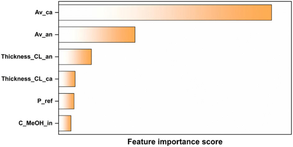 | ||
| Fig. 6 Average feature importance prediction plots based on the best ETR models in ten-fold cross-validation (top 6). | ||
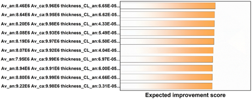 | ||
| Fig. 7 The EI score of the top 10 combinations obtained through ML. | ||
In order to test the learning results of SMAC, we brought the 10 groups of parameters with the highest expected improvement value into the model and performed numerical simulation to obtain their I–V polarization curves and compared them with the polarization curves of the first and second power density in the original database. As shown in Fig. 8, compared with the original database, more than half of the polarization curves obtained by the top 10 parameter combinations with the EI score exceeded the maximum power density of the original database.
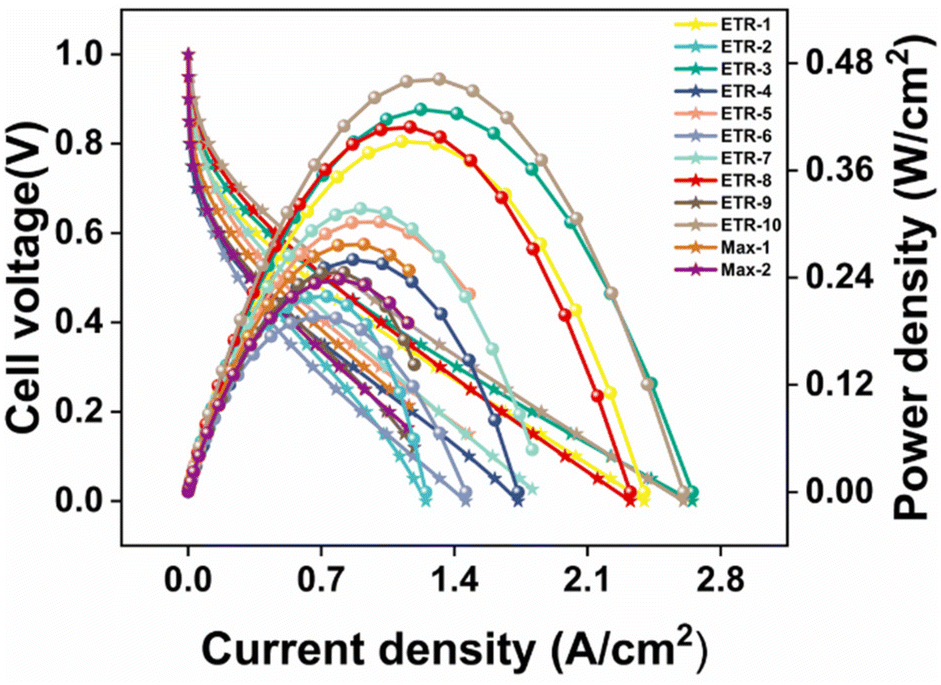 | ||
| Fig. 8 Comparison between the top 10 EI score data and the polarization curve of the original database. | ||
The model we have established has the ability to capture dynamic effects. As shown in the ESI Movie S1,† it illustrates the concentration change process of methanol in the cathode of a methanol fuel cell. It can be seen that methanol diffuses in the flow field and reacts with GDL after coming into contact with the catalytic layer. The concentration of methanol decreases sequentially from the fuel inlet to the outlet, from the middle to both sides. To explore the internal mechanism of the performance improvement, we selected the optimal parameter combination to analyse the distribution of the reactants and products. Compared with the initial parameters, the thickness of the cathode catalytic layer, the flow rate of the channel, the permeability and the specific surface area of the cathode and anode all increase.65,66 Compared with the initial parameters, the thickness of the cathode catalytic layer, the channel flow rate of the cathode anode, the permeability and specific surface area of the catalytic layer, as well as the temperature and pressure of the anode catalytic layer all increased, while the thickness of the anode catalytic layer decreased, as shown in Fig. 9. Due to the increase in the anode inlet velocity and the increase in permeability, the distribution of methanol concentration was more uniform than that in the initial model (Fig. S1†). When the cell voltage is 0.35 V (maximum power density voltage), the methanol concentration drops from 224.8 mol m−3 to 216.3 mol m−3, which is greater than 2.1 mol m−3 of the initial model. The effect of height and high pressure, as well as the increase in the specific surface area of the anode, make methanol oxidation more thorough.67 The thinner anode catalytic layer also helps reduce methanol penetration. The distribution of CO2 is completely opposite to that of methanol, which also proves that the methanol reaction is sufficient. The same explanation applies to oxygen and water concentrations. The above conclusions show that the parameter combinations recommended by ML can significantly improve methanol fuel cells, and the ideas provided in this paper also provide new insights into the optimization direction of DMFC.
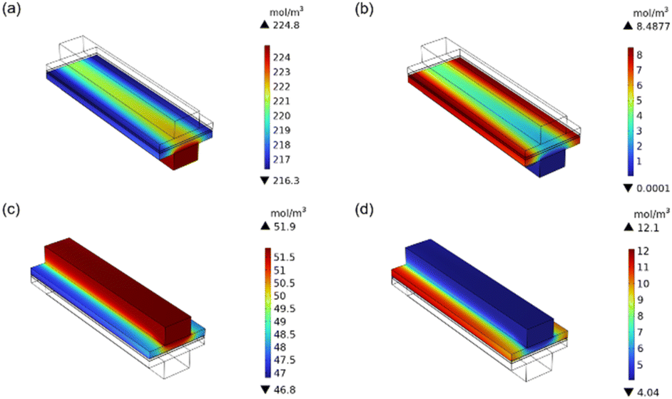 | ||
| Fig. 9 The concentration distribution of reactants and products (0.35 V) was predicted by the optimal parameter combination: (a) molar concentration of methanol at the anode, (b) molar concentration of CO2 at the anode, (c) molar concentration of oxygen at the cathode, and (d) molar concentration of water at the cathode. | ||
4 Conclusions
In this study, we combined numerical simulation and ML high throughput to reveal the effects of different parameters of CL on the DMFC performance. First, the optimized models were obtained by training 7 ML algorithms on the database. Then, a comprehensive tree-based regression model (XGB, ETR, and RFR) was used to rank the importance of the 19 complex eigenvalues, and the input eigenvariables with the greatest influence were quantitatively determined. The results of these three algorithms all show the same first three important characteristic values: cathode specific surface area, anode specific surface area and anode thickness. Then, SMAC was used to get the expected improved values of different parameter combinations. The top ten parameter combinations with EI score were selected and imported into the simulation model for testing, and the entire output I–V polarization curve of the DMFC was obtained and compared with the I–V polarization curve of the maximum power density in the original database. The results show that a majority of the polarization curves obtained from the top combinations exceed the maximum power density of the original database.We provide a method that leverages simulation models to rapidly establish databases and integrates machine learning to accelerate parameter optimization. However, to reduce computational complexity and enhance simulation efficiency, we simplified the fuel cell system to a certain extent. Real fuel cell operating conditions are influenced by factors across multiple scales, including the microscale (such as electrode material structure, and catalyst layer activity), mesoscale (such as flow channel design and gas diffusion layer structure), and macroscale (such as overall cell structure and thermal management design). Yet, overly complex models can incur significant computational costs. Additionally, there is often a contradiction between the real-time performance and accuracy of models. To improve the real-time performance, models may need to be simplified or their precision reduced, whereas to enhance accuracy, model complexity and computational load need to be increased. Currently, the concept of digital twins is rapidly gaining popularity, aiming to create virtual replicas of physical entities for data interaction with the actual objects and utilizing machine learning to train data-driven surrogate models based on datasets. The developed surrogate models are expected to offer accuracy comparable to multi-physics predictive physical models while possessing response speeds much faster than those of simulation models. Currently, digital twins have been widely applied in complex systems of various scales, including cities, factories, and airplanes.68–70 This technology, characterized by high interactivity and rapid optimization iteration,71,72 can address the aforementioned issues. This work lays the foundation for the establishment of a digital twin model for direct methanol fuel cells. In the future, by training surrogate models, rapid interaction between fuel cell entities and digital models can be achieved, effectively determining and monitoring their multi-physics field states. This has significant implications for fuel cell design and control operations.
Author contributions
Lishou Ban: methodology, formal analysis, writing – original draft. Danyang Huang: conceptualization, data curation. Yanyi Liu: investigation, validation. Pengcheng Liu: software, writing – review & editing. Xihui Bian and Yifan Liu: supervision, resources. Kaili Wang: supervision, writing – review & editing. Xijun Liu: supervision, resources. Jia He: conceptualization, project administration, funding acquisition.Data availability
The authors will supply the relevant data in response to reasonable requests.Conflicts of interest
The authors declare that they have no known competing financial interests or personal relationships that could have appeared to influence the work reported in this paper.Acknowledgements
This work was financially supported by the National Natural Science Foundation of China (52073214) and the Shenzhen Science and Technology Program (JCYJ20230807112503008). This research was supported by TianHe Qingsuo Open Research Fund of TSYS in 2022 & NSCC-TJ.References
- Y. J. Wang, J. Qiao, R. Baker and J. Zhang, Chem. Soc. Rev., 2013, 42, 5768 RSC.
- M. M. Mohideen, A. V. Radhamani, S. Ramakrishna, Y. Wei and Y. Liu, J. Energy Chem., 2022, 69, 466 CrossRef CAS.
- J. Zhou, H. Xiao, W. Weng, D. Gu and W. Xiao, J. Energy, Chem., 2020, 50, 280 CrossRef.
- W. R. W. Daud, R. E. Rosli, E. H. Majlan, S. A. A. Hamid, R. Mohamed and T. Husaini, Renewable Energy, 2017, 113, 620 CrossRef CAS.
- Z. Shangguan, B. Li, P. Ming and C. Zhang, J. Mater. Chem., 2021, 9, 15111 RSC.
- Y. H. Shen, H. Lv, Y. Q. Hu, J. W. Li, H. Lan and C. M. Zhang, Renewable Energy, 2023, 212, 834 CrossRef CAS.
- H. Mistry, A. S. Varela, S. Kuhl, P. Strasser and B. R. Cuenya, Nat. Rev. Mater., 2016, 1, 16009 CrossRef CAS.
- L. Fu, W. Ji, J. He, C. Huang, Y. Li and Y. Dou, China Powder Sci. Technol., 2024, 30, 170 Search PubMed.
- F. Lyu, M. Cao, A. Mahsud and Q. Zhang, J. Mater. Chem., 2020, 8, 15445 RSC.
- E. P. Murray, T. Tsai and S. A. Barnett, Nature, 1999, 400, 649 CrossRef CAS.
- J. Zhao, H. Y. Liu and X. G. Li, Electrochem. Energy Rev., 2023, 6, 13 CrossRef CAS PubMed.
- P. C. Sui, X. Zhu and N. Djilali, Electrochem. Energy Rev., 2019, 2, 428 CrossRef CAS.
- S. Q. Song, W. J. Zhou, W. Z. Li, G. Sun, Q. Xin, S. Kontou and P. Tsiakaras, Ionics, 2004, 10, 458–462 CrossRef CAS.
- S. Arisetty, C. A. Jacob, A. K. Prasad and S. G. Advani, J. Power Sources, 2009, 187, 415 CrossRef CAS.
- S. H. Seo and C. S. Lee, Appl. Energy, 2010, 87, 2597 CrossRef CAS.
- S. H. Yang, C. Y. Chen and W. J. Wang, J. Power Sources, 2010, 195, 2319 CrossRef CAS.
- S. Chen, F. Ye and W. Lin, Int. J. Hydrogen Energy, 2010, 35, 8225 CrossRef CAS.
- I. Taymaz, F. Akgun and M. Benli, Energy, 2011, 36, 1155 CrossRef CAS.
- A. Jason, J. A. Varnell, J. S. Sotiropoulos, T. M. Brown, K. Subedi, R. T. Haasch, C. E. Schulz and A. A. Gewirth, ACS Energy Lett., 2018, 3, 823 CrossRef.
- F. Jaouen, M. Lefèvre, J. P. Dodelet and M. Cai, J. Phys. Chem. B, 2006, 110, 5553 CrossRef CAS.
- N. D. Leonard, K. Artyushkova, B. Halevi, A. Serov, P. Atanassov and S. C. Barton, J. Electrochem. Soc., 2015, 162, F1253 CrossRef CAS.
- J. C. Park, S. H. Park, M. W. Chung, C. H. Choi, B. K. Kho and S. I. Woo, J. Power Sources, 2015, 286, 166 CrossRef CAS.
- Y. Yin, J. Liu, Y. F. Chang, Y. Z. Zhu, X. Xue, Y. Z. Qin, J. F. Zhang, K. Jiao, Q. Du and M. D. Guiver, Electrochim. Acta, 2019, 296, 450 CrossRef CAS.
- Q. Yang, A. Kianimanesh, T. Freiheit, S. S. Park and D. Xue, J. Power Sources, 2011, 196, 10640 CrossRef CAS.
- B. Yu, Q. Yang, A. Kianimanesh, T. Freiheit, S. S. Park, H. Zhao and D. Xue, Int. J. Hydrogen Energy, 2013, 38, 9873 CrossRef CAS.
- M. Tafaoli-Masoule, A. Bahrami and E. M. Elsayed, Energy, 2014, 70, 643 CrossRef.
- J. Lee, S. Lee, D. Han, G. Gwak and H. Ju, Int. J. Hydrogen Energy, 2017, 42, 1736 CrossRef CAS.
- J. Jiang, Y. Li, J. Liang, W. Yang and X. Li, Appl. Energy, 2019, 252, 113431 CrossRef CAS.
- M. S. Hossain and G. Muhammd, Inf. Fusion, 2019, 49, 69 CrossRef.
- C. Shan, S. Gong and P. W. Mcowan, Image Vis. Comput., 2009, 27, 803 CrossRef.
- J. Cao, T. Chen and J. Fan, Multimed. Tools Appl., 2016, 75, 2839 CrossRef.
- W. Lou, A. Ali and P. K. Shen, Nano Res., 2022, 15, 18–37 CrossRef CAS.
- W. Lei, M. Li, L. He, X. Meng, Z. Mu, Y. Yu, F. M. Ross and W. W. Yang, Nano Res., 2020, 13, 638 CrossRef CAS.
- J. Ruan, Y. Chen, G. Zhao, P. Li, B. Zhang, Y. Jiang, T. Y. Ma, H. G. Pan, S. X. Dou and W. P. Sun, Small, 2022, 2107067 CrossRef CAS.
- H. Li, Y. Pan, D. Zhang, Y. Han, Z. Wang, Y. Qin, S. Y. Lin, X. K. Wu, H. Zhao, J. P. Lai, B. L. Huang and L. Wang, J. Mater. Chem., 2020, 8, 2323 CAS.
- H. Ooka, J. Huang and K. S. Exner, Front. Energy Res., 2021, 9, 654460 Search PubMed.
- V. Stamenkovic, B. S. Mun, K. J. J. Mayrhofer, P. N. Ross, N. M. Markovic, J. Rossmeisl, J. Greeley and J. K. Nørskov, Angew. Chem., Int. Ed., 2006, 45, 2897 CrossRef CAS PubMed.
- L. Zhang, P. Lu, M. Yin, R. Li, B. Wang, X. Ma, M. Jiao, W. Ma and Z. Zhou, Rare Met., 2024 DOI:10.1007/s12598-024-03039-3.
- W. Y. Ming, P. Y. Sun, Z. Zhang, W. Z. Qiu, J. G. Du, X. K. Li, Y. M. Zhang, G. J. Zhang, K. Liu, Y. Wang and X. D. Guo, Int. J. Hydrogen Energy, 2023, 48, 5197 CrossRef CAS.
- R. Ding, R. Wang, Y. Ding, W. J. Yin, Y. D. Liu, J. Li and J. G. Liu, Angew. Chem., 2020, 132, 19337 CrossRef.
- R. Ding, W. J. Yin, G. Cheng, Y. W. Chen, J. K. Wang, X. B. Wang, M. Han, T. R. Zhang, Y. L. Cao, H. M. Zhao, S. P. Wang, J. Li and J. G. Liu, ACS Appl. Mater., 2022, 14, 8010 CrossRef CAS.
- N. S. Vasile, A. H. A. M. Videla and S. Specchia, Chem. Eng. J., 2017, 322, 722 CrossRef CAS.
- P. T. Sun, S. Zhou, Q. Y. Hu and G. P. Liang, Commun. Comput. Phys., 2012, 11, 65–98 CrossRef.
- K. Suzuki, T. Toyao, Z. Maeno, S. Takakusagi, K. Shimizu and I. Takigawa, ChemCatChem, 2019, 11, 4537 CrossRef CAS.
- X. Liu, M. Chen, J. Ma, J. Liang, C. Li, C. Chen and H. He, China Powder Sci. Technol., 2024, 30, 35 Search PubMed.
- F. Wang, C. Kuang, Z. Zheng, D. Wu, H. Wan, G. Chen, N. Zhang, X. Liu and R. Ma, Chin. Chem. Lett., 2024, 109989 CrossRef.
- Y. Ji, Z. Yu, L. Yan and W. Song, China Powder Sci. Technol., 2023, 29, 100 Search PubMed.
- W. Liu, W. Liu, T. Hou, J. Ding, Z. Wang, R. Yin, X. San, L. Feng, J. Luo and X. Liu, Nano Res., 2024, 17, 4797 CrossRef CAS.
- J. Ding, S. Jing, C. Yin, C. Ban, K. Wang, X. Liu, Y. Duan, Y. Zhang, G. Han, L. Gan and J. Rao, Chin. Chem. Lett., 2023, 34, 107899 CrossRef CAS.
- J. Li, S. Yan, G. Li, Y. Wang, H. Xu and G. Duan, China Powder Sci. Technol., 2023, 29, 101 Search PubMed.
- T. Onsree and N. Tippayawong, Renewable Energy, 2021, 167, 425 CrossRef CAS.
- Q. J. Song, H. Y. Jiang and J. Liu, Expert Syst. Appl., 2017, 81, 22 CrossRef.
- H. K. Esfeh, A. Azarafza and M. K. A. Hamid, RSC Adv., 2017, 7, 32893 RSC.
- J. Sun, G. Zhang, T. Guo, G. B. Che, K. Jiao and X. R. Huang, Appl. Therm. Eng., 2020, 165, 114589 CrossRef CAS.
- M. Tian, S. Shi, Y. Shen and H. M. Yin, Electrochim. Acta, 2019, 293, 390 CrossRef CAS.
- I. Blankenau, L. Marten and X. Li, ECS Meet. Abstr., 2019, 36, 1677 CrossRef.
- C. C. Ngetich, J. Mutua, P. Kareru, K. Karanja and E. Wanjuru, Fuel Cells, 2023, 23, 324–337 CrossRef CAS.
- Z. G. Zhao, D. J. Li, X. P. Xu and D. C. Zhang, Energies, 2023, 16, 2167 CrossRef CAS.
- D. E. Glass and G. K. S. Prakash, Electroanalysis, 2019, 31, 718 CrossRef CAS.
- D. E. Glass, G. A. Olah and G. K. S. Prakash, J. Power Sources, 2017, 352, 165 CrossRef CAS.
- X. H. Yan, P. Gao, G. Zhao, L. Shi, J. B. Xu and T. S. Zhao, Appl. Therm. Eng., 2017, 126, 290 CrossRef CAS.
- Z. Chen, S. Mak, C. F. J. Wu and J. Am, Stat. Assoc., 2023, 1–14 Search PubMed.
- J. Yang, F. Zhang and J. Chen, China Powder Sci. Technol., 2024, 30, 161 Search PubMed.
- K. Chen, D. Ma, Y. Zhang, F. Wang, X. Yang, X. Wang, H. Zhang, X. Liu, R. Bao and K. Chu, Urea Adv. Mater., 2024, 36, 2402160 CrossRef CAS.
- A. Fumiaki and T. Keisuke, Energy Mater., 2024, 4, 400006 Search PubMed.
- G. Lu, G. Meng, Q. Liu, L. Feng, J. Luo, X. Liu, Y. Luo and P. K. Chu, Adv. Powder Mater., 2024, 3, 100154 CrossRef.
- S. Chen, G. Qi, R. Yin, Q. Liu, L. Feng, X. Feng, G. Hu, J. Luo, X. Liu and W. Liu, Nanoscale, 2023, 15, 19577 RSC.
- B. W. Wang, G. B. Guo, H. Z. Wang, J. Xuan and K. Jiao, Energy AI, 2020, 1, 100004 CrossRef.
- X. Kang, Y. J. Wang, C. Jiang and Z. H. Cheng, Batteries, 2024, 10, 242 CrossRef CAS.
- H. Kim, S. Hong, J. Bang, Y. Jun, S. Choe, S. Kim and S. Ahn, Energy Mater., 2024, 4, 400010 CAS.
- B. He, Y. Ling, Z. Wang, W. Gong, Z. Wang, Y. Liu, T. Zhou, T. Xiong, S. Wang, Y. Wang, Q. Li, Q. Zhang and L. Wei, eScience, 2024, 4, 100293 CrossRef.
- H. Fan, K. Liu, X. Zhang, Y. Di, P. Liu, J. Li, B. Hu, H. Li, M. Ravivarma and J. Song, eScience, 2024, 4, 100202 CrossRef.
Footnotes |
| † Electronic supplementary information (ESI) available. See DOI: https://doi.org/10.1039/d4nr03026e |
| ‡ These authors contributed equally to this work. |
| This journal is © The Royal Society of Chemistry 2025 |